A Composite Barrier Function Sliding Mode Control Method Based on an Extended State Observer for the Path Tracking of Unmanned Articulated Vehicles

Abstract

Unmanned articulated vehicles play a crucial role in the intelligent mine system and have been extensively investigated and implemented in the fields of mine transportation, agriculture and forestry construction. However, the working environment of articulated wheeled vehicles is harsh and the working conditions are changeable. These conditions are often accompanied by load changes, road interference excitation caused by an unstructured environment and the dynamic nonlinear characteristics of articulated wheeled vehicles. The current research on path tracking control methods suitable for traditional wheeled vehicles does not meet the intelligent operation requirements of articulated wheeled vehicles, and it is necessary to combine the specific working environment and its own specific structural model characteristics. In this paper, a composite barrier function sliding mode control method based on an extended state observer is proposed to solve the problem of modeling uncertainty and unknown external disturbance in the path tracking control of unmanned articulated vehicles. Firstly, the mathematical model of the articulated wheeled working vehicle is built to derive the expected heading angle in the prediction horizon. Then, the strong nonlinear lumped disturbance in articulated dynamics is dynamically estimated by combining the composite nonlinear extended state observer. Afterward, based on the error compensation theory, a composite barrier function sliding mode controller suitable for articulated vehicle path tracking is derived. Finally, through simulation analysis and experimental verification, this method can estimate the strong nonlinear lumped disturbance caused by the structural characteristics of the articulated vehicle, and then compensate for the disturbance of the control quantity to achieve stable, robust and accurate path tracking control.

1. Introduction

In complex unstructured environments, the working environments of articulated special transport vehicles are mostly uneven road surfaces, and there are many irregular obstacles (sand, mound, etc.). Whether these vehicles can efficiently and safely cross or avoid obstacles in the working space is the primary problem that must be considered in path planning and tracking control [1,2,3]. Moreover, due to the kinematic characteristics brought about by the articulated steering structure, the nonholonomic constraints of the system are added [4]. Due to the highly nonlinear nature of the system [5], the backward motion of the articulated vehicle is unstable, so the path tracking method suitable for traditional vehicles cannot fully consider its unique articulated steering structural characteristics.

Path tracking control is the key link to achieving the autonomous operation system of unmanned articulated vehicles. Its core task is to control the actuator motion through the path tracking controller according to the current vehicle state of the articulated vehicle, combined with the dynamic characteristics of the vehicle, according to the path information calculated by the path planning module, so that the actual path of the vehicle, the state of the vehicle and other dynamic indicators are consistent with the reference path, ensuring that the vehicle can drive stably and safely along the planned path. The main difference between the articulated wheeled vehicle and the traditional wheeled vehicle is the steering mode [6]. The articulated wheeled vehicle adopts the articulated structure to steer. Therefore, the traditional path tracking method cannot realize the path tracking control of the articulated wheeled vehicle. In addition, the articulated wheeled vehicle works in harsh and changeable working conditions [7], which are often accompanied by load changes, road interference excitation caused by an unstructured environment, and the dynamic nonlinear characteristics of the articulated wheeled vehicle itself.

In recent years, many scholars have conducted a lot of research on path tracking algorithms and have achieved rich research results. At present, the main path tracking control algorithms are mainly divided into the classical control method, geometric motion control method, optimal theory control method and model predictive control method. Chen et al. [8] proposed a lateral and longitudinal coupling controller based on the model predictive control framework to realize the lateral and longitudinal coupling control of the path tracking of autonomous vehicles. The proportional integral derivative (PID) controller achieves longitudinal control, which is mainly responsible for controlling the driving and braking functions of the vehicle. Yang et al. [9] proposed a path tracking algorithm based on the optimal target point. The algorithm simulates the driver’s look-ahead behavior and searches the optimal target point according to the evaluation function in the look-ahead area to achieve path tracking accuracy in the automatic navigation of agricultural machinery. This algorithm solves the problem of selecting the best look-ahead point in the traditional pure tracking algorithm. Zhang et al. [10] proposed a tracking control method based on particle swarm optimization linear quadratic regulator (PSO-LQR). By optimizing the weight matrix of LQR by PSO, a PSO-LQR controller with feedforward control is designed, which improves the tracking accuracy and vehicle stability. Yuan et al. [11] proposed a trajectory tracking controller that combines LQR and model predictive control. The controller can simultaneously minimize the lateral tracking deviation and track the desired trajectory and vehicle speed, improving the robustness of the overall controller framework. Sun et al. [12] designed an integrated path tracking controller for articulated vehicles to verify the tracking performance at different reference speeds. The upper controller is used to solve the longitudinal speed and steering rate of the vehicle, and the lower controller converts the upper solution into the signal of the vehicle actuator. Chen et al. [13] proposed a novel fuzzy logic switched model predictive control algorithm to solve the path tracking challenge caused by road conditions and vehicle speed changes for articulated steering vehicles. Because the articulated vehicle adopts the articulated steering mode, it needs to be improved according to the control requirements and the unique dynamic characteristics of the articulated vehicle in the specific application. It can be seen that the path planning algorithm and path tracking control method suitable for traditional wheeled vehicles cannot meet the intelligent operation requirements of unmanned articulated wheeled vehicles. It is necessary to study the path planning and path tracking technology of the unique articulated wheeled vehicle configuration in combination with the specific operating environment and its own specific structural model characteristics. Therefore, research on path planning and tracking control of articulated wheeled vehicles is of great value and significance for improving the intelligence of engineering vehicles and the efficiency of engineering construction.

In this paper, an articulated vehicle path tracking control method based on extended state observer-based composite barrier function sliding mode control is proposed. The overall framework is shown in Figure 1. Firstly, the mathematical model of the articulated wheeled working vehicle is built, and the path tracking control model is derived based on the comprehensive expected heading angle. In Figure 1a, this step serves to calculate the combined desired yaw angle and total disturbances, which are subsequently transmitted to the observer. Secondly, an extended state observer with stable convergence is designed to observe and estimate the total disturbance and state variables of the system. The composite barrier function is used as the gain of the sliding mode controller, and the control gain can be adaptively adjusted according to the sliding variable. In Figure 1b,c, this step involves combining CNESO with an adaptive sliding mode controller based on barrier function to design the composite barrier function sliding mode controller. Moreover, the co-simulation environment shown in Figure 1d is built to verify that the composite barrier function sliding mode controller has a better control effect and lower control input chattering. Finally, based on the robot operating system (ROS) platform, a prototype of an articulated test principle is built to verify various test conditions. The experimental results show that the path planning tracking control method proposed in this paper has the advantages of strong applicability and robustness.

2. Modeling of Mathematical Model and Path Tracking Error Model

2.1. Nonlinear Kinematics and Dynamics Model of Unmanned Articulated Vehicle

2.1.1. Modeling of Kinematics for Unmanned Articulated Vehicle

The kinematic characteristics of the unmanned articulated vehicle are very different from those of the rigid passenger vehicle during the steering process. As shown in Figure 2, the front and rear vehicle bodies are connected by the articulated mechanism and have the special driving characteristics of the articulated point steering.

The derivation of the kinematic model of the unmanned articulated vehicle is given in [13]. The vehicle’s nonlinear state-space system can be expressed as a matrix form:

$$\left[\begin{array}{c}{\stackrel{·}{x}}_f\\ {\stackrel{·}{y}}_f\\ {\stackrel{·}{\theta }}_f\\ \stackrel{·}{\beta }\end{array}\right]=\left[\begin{array}{cc}\cos {\theta }_f& 0\\ \sin {\theta }_f& 0\\ {\displaystyle \frac{\sin \beta }{L_f\cos \beta +L_r}}& {\displaystyle \frac{L_r}{L_f\cos \beta +L_r}}\\ 0& 1\end{array}\right]\left[\begin{array}{c}{v}_f\\ \stackrel{·}{\beta }\end{array}\right]$$

(1)

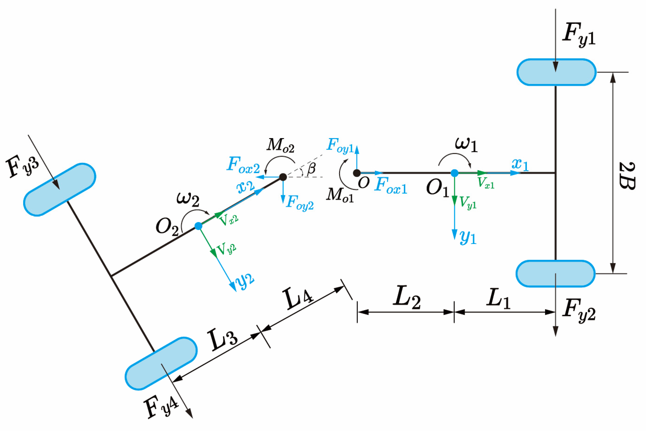
2.1.2. Nonlinear Dynamic Model of Unmanned Articulated Vehicle

A mechanical analysis of the 3-DOF model of the articulated vehicle is shown in Figure 3. The articulated vehicle adopts a special articulated structure for steering. Therefore, the steering torque can be applied to the front and rear vehicle bodies by controlling the hinged device in the middle, so as to control the overall steering of the articulated vehicle. In the whole process of model establishment, the following assumptions are made for the vehicle [14]:

• The front and rear vehicle bodies are rigid bodies, ignoring the influence of force on the deformation of the vehicle body.
• The centroids of the front and rear vehicle bodies are located on the longitudinal center axis, and the vehicle is symmetrical about the longitudinal center axis.
• The influences of tire camber angle and aligning torque on the dynamic characteristics of the wheel are ignored.
• Air resistance is ignored, and the road surface is flat.

According to Newton’s second law and Euler’s second law, the 3-DOF model formula of the articulated vehicle can be obtained as follows:

$$\left\{\begin{array}{c}{m}_1{a}_{y1}+m_2{a}_{y2}=F_{y1}+F_{y2}+F_{y3}+F_{y4}\\ \left(I_1+m_1{L}_2^2\right){\stackrel{·}{\omega }}_1=M+\left(F_{y1}+F_{y2}\right)\left(L_1+L_2\right)\\ \left(I_2+m_2{L}_3^2\right){\stackrel{·}{\omega }}_2=-M-\left(F_{y3}+F_{y4}\right)\left(L_3+L_4\right)\end{array}\right.$$

(2)

In the formula, ${\omega }_1$, ${\omega }_2$ are the yaw rate of the front and rear vehicle bodies; $m_1$, $m_2$ are the mass of the front and rear vehicle bodies; and $I_1$, $I_2$ are the moment of inertia of the front and rear vehicle bodies around $O_1{z}_1,O_2{z}_2$.

Assuming and considering the relative yaw motion of the front and rear vehicle bodies, and that the front and rear vehicle bodies are connected by hinge points, it can be obtained that

$$\begin{array}{l}{a}_{y1}={\stackrel{·}{v}}_{y1}+v_{x1}{\omega }_1\\ a_{y2}={\stackrel{·}{v}}_{y1}-\left(L_2+L_3\right){\stackrel{·}{\omega }}_1+L_3\stackrel{··}{\beta }+v_{x1}\stackrel{·}{\beta }+v_{x2}{\omega }_2\end{array}$$

(3)

The angle of the waist changes into

$$\stackrel{·}{\beta }={\omega }_1-{\omega }_2$$

(4)

Since the dynamic model is mainly used for the construction of control formulas, some formulas are linearized. The tire model uses a linear tire model, and the tire linearization model is shown as follows:

$$F_{yi}=C_{{\mathrm{\alpha }}_i}{\alpha }_i$$

(5)

In the formula, $C_{{\alpha }_i}$ is the tire cornering stiffness and ${\alpha }_i$ is the tire cornering angle during vehicle driving. The sideslip angle can be expressed as follows:

$$\left\{\begin{array}{c}{\alpha }_{fi}={\displaystyle \frac{v_{y1}+L_1{\omega }_1}{v_x}}\\ a_{ri}={\displaystyle \frac{v_{y1}-\left(L_2+L_3+L_4\right){\omega }_1+\left(L_3+L_4\right)\stackrel{·}{\beta }+v_{x1}\beta }{v_x}}\end{array}\right.$$

(6)

By substituting the lateral velocity and yaw rate of the eliminated vehicle body into the combined Formulas (6)–(10), the dynamic model formula based on the front vehicle body can be obtained as follows:

$$\left[\begin{array}{c}{\stackrel{·}{v}}_{y1}\\ {\stackrel{·}{\omega }}_1\end{array}\right]=\left[\begin{array}{cc}{a}_{11}& a_{12}\\ a_{21}& a_{22}\end{array}\right]\left[\begin{array}{c}{v}_{y1}\\ {\omega }_1\end{array}\right]+\left[\begin{array}{c}{a}_{13}\\ a_{23}\end{array}\right]\stackrel{·}{\beta }+\left[\begin{array}{c}{a}_{14}\\ a_{24}\end{array}\right]\beta +\left[\begin{array}{c}{a}_{15}\\ a_{25}\end{array}\right]M$$

(7)

In the formula,

$$\begin{array}{l}{a}_{11}={\displaystyle \frac{2m_2{L}_2\left(L_1+L_2\right)C_{\alpha f}}{\left(m_1+m_2\right)\left(I_1+m_1{L}_2^2\right)V_x}}-{\displaystyle \frac{2C_{\alpha r}\left(L_3+L_4\right)m_2{L}_3}{\left(m_1+m_2\right)\left(I_2+m_2{L}_3^2\right)V_x}}+{\displaystyle \frac{2\left(C_{\alpha f}+C_{\alpha r}\right)}{\left(m_1+m_2\right)V_x}}\\ a_{12}={\displaystyle \frac{2m_2\left(L_1+L_2\right)C_{\alpha f}{L}_1{L}_2}{\left(m_1+m_2\right)\left(I_1+m_1{L}_2^2\right)V_x}}+{\displaystyle \frac{2C_{\alpha f}{L}_1-2C_{\alpha r}\left(L_2+L_3+L_4\right)}{\left(m_1+m_2\right)V_x}}+{\displaystyle \frac{2C_{\alpha r}\left(L_3+L_4\right)\left(L_2+L_3+L_4\right)m_2{L}_3}{\left(I_2+m_2{L}_3^2\right)\left(m_1+m_2\right)V_x}}-V_x\\ a_{21}={\displaystyle \frac{2\left(L_1+L_2\right)C_{\alpha f}}{\left(I_1+m_1{L}_2^2\right)V_x}} a_{22}={\displaystyle \frac{2\left(L_1+L_2\right)C_{\alpha f}{L}_1}{\left(I_1+m_1{L}_2^2\right)V_x}} a_{13}={\displaystyle \frac{2C_{\alpha r}\left(L_3+L_4\right)}{V_x\left(m_1+m_2\right)}}-{\displaystyle \frac{2C_{\alpha r}{\left(L_3+L_4\right)}^2{m}_2{L}_3}{\left(I_2+m_2{L}_3^2\right)\left(m_1+m_2\right)}}\\ a_{23}=0 a_{14}={\displaystyle \frac{2C_{\alpha r}}{m_1+m_2}}-{\displaystyle \frac{2C_{\alpha r}\left(L_3+L_4\right)m_2{L}_3}{\left(m_1+m_2\right)\left(I_2+m_2{L}_3^2\right)}} a_{24}=0\\ a_{15}={\displaystyle \frac{m_2{L}_2}{\left(I_1+m_1{L}_2^2\right)\left(m_1+m_2\right)}}-{\displaystyle \frac{m_2{L}_3}{\left(I_2+m_2{L}_3^2\right)\left(m_1+m_2\right)}} a_{25}={\displaystyle \frac{1}{I_1+m_1{L}_2^2}}\end{array}$$

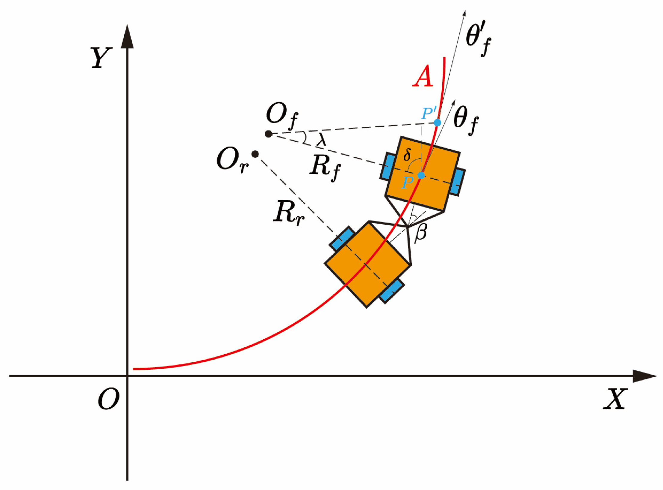
2.2. Path Tracking Error Model

In the path tracking control problem of articulated vehicles, eliminating the path tracking error is the goal of control system design, and it is also a problem that has always been concerned in the research of the path tracking problem.

2.2.1. Path Tracking Expected Heading Angle

The dynamic model of an articulated vehicle is a typical underactuated system. By reducing the dimension of the system, the complexity of control can be effectively reduced. We can achieve the following control of the reference path by tracking the required heading angle. The path tracking error model of an articulated vehicle in the Serret–Frenet coordinate system is shown in Figure 4. In Figure 4, α is the vehicle’s sideslip angle, which can be estimated by a variety of estimation methods [15,16]. When the front body of the articulated vehicle is above the reference path, $Z_e$ is positive, while $Z_e$ is negative below the reference path.

Let ${\phi }_e=\phi -{\phi }_{ref}$, and control the lateral displacement deviation $Z_e$ and the heading angle deviation ${\phi }_e$ to converge to zero, so that the articulated vehicle follows the given reference path for the driving operation. Through coordinate transformation, we can obtain the motion error formula of the Serret–Frenet framework as follows:

$$\begin{array}{l}{\stackrel{·}{z}}_e=v_x\sin {\phi }_e+v_y\cos {\phi }_e\\ {\stackrel{·}{\phi }}_e={\omega }_r-{\displaystyle \frac{c\left(s\right)}{1-c\left(s\right)z_e}}\left(v_x\cos {\phi }_e-v_y\sin {\phi }_e\right)\\ \stackrel{·}{s}={\displaystyle \frac{1}{1-c\left(s\right)z_e}}\left(v_x\cos {\phi }_e-v_y\sin {\phi }_e\right)\end{array}$$

(8)

In this formula, (s) is the curvature of the M point on the reference path R; using the Serret–Frenet framework, we can derive the following:

$${\stackrel{·}{z}}_e=\sqrt{v_x^2+v_y^2}\sin \left({\phi }_e+\alpha \right)$$

(9)

2.2.2. Comprehensive Expected Heading Angle in Prediction Horizon

In the process of path tracking control, external disturbances such as road curvature have an impact on the actual effect of path tracking. Preview control [17] is an important solution for solving disturbances like road curvature. Using dead reckoning technology, and according to the pose information of the current vehicle, the future vehicle pose in a certain horizon is estimated. During the path tracking process, road curvature information is incorporated. Combined with the expected heading angle of path tracking proposed above, a comprehensive expected heading angle, considering road curvature information in the prediction horizon, is obtained. It can improve the response speed of an articulated vehicle in path tracking control for road curvature and other factors. The driving curve of an articulated vehicle within the prediction horizon is shown in Figure 5.

Through analysis of a kinematic model of an articulated vehicle, the change rate of heading angle of front vehicle body is as follows:

$${\stackrel{·}{\theta }}_f={\displaystyle \frac{v_f\sin \beta +\stackrel{·}{\beta L_r}}{L_f\cos \beta +L_r}}$$

(10)

The time interval in the prediction horizon is $∆t$, and smaller time interval is usually used. Therefore, it can be assumed that the change rate of the heading angle remains unchanged during the time interval. As a result, the heading angle relationship between current moment and next moment can be obtained as follows:

$${\theta }_f^{\prime }={\theta }_f+{\stackrel{·}{\theta }}_f\Delta t={\theta }_f+{\displaystyle \frac{v_f\sin \beta +L_r\stackrel{·}{\beta }}{L_f\cos \beta +L_r}}\Delta t$$

(11)

According to a kinematics analysis of the vehicle, the steering radius of the front vehicle body is as follows:

$$F_{yi}=C_{{\mathrm{\alpha }}_i}{\alpha }_i$$

(12)

In a single time interval, the steering angular velocity of the front body moving from point P (x, y) to point P′ (x, y) is ${\omega }_f$. Therefore, the turning angle of the front vehicle body is as follows:

$$R_f={\displaystyle \frac{v_f\left(L_r+L_f\cos \beta \right)}{v_f\sin \beta +L_r\stackrel{·}{\beta }}}$$

(13)

According to the geometric relationship of motion, the moving distance of vehicle body is as follows:

$$l_{p{p}^{\prime }}=2R_f\sin {\displaystyle \frac{\lambda }{2}}$$

(14)

Thus, it can be calculated that the midpoint coordinate P′ (x, y) of the vehicle body before the next moment is as follows:

$$x^{\prime }=\left\{\begin{array}{c}x+v_f\Delta t\cos {\theta }_f\left({\theta }_f={\theta }_f^{\prime }\right)\\ x+l_{P{P}^{\prime }}\cos \delta \left(0<{\theta }_f<{\displaystyle \frac{\pi }{2}}\right)\\ x-l_{P{P}^{\prime }}\cos \delta \left({\displaystyle \frac{\pi }{2}}\le {\theta }_f\le \pi \right)\\ x+l_{P{P}^{\prime }}\cos \delta \left(-{\displaystyle \frac{\pi }{2}}\le {\theta }_f\le 0\right)\\ x-l_{P{P}^{\prime }}\cos \delta \left(-\pi <{\theta }_f\le -{\displaystyle \frac{\pi }{2}}\right)\end{array}\right.y^{\prime }=\left\{\begin{array}{c}y+v_f\Delta t\cos {\theta }_f\left({\theta }_f={\theta }_f^{\prime }\right)\\ y+l_{P{P}^{\prime }}\sin \delta \left(0<{\theta }_f<{\displaystyle \frac{\pi }{2}}\right)\\ y+l_{P{P}^{\prime }}\sin \delta \left({\displaystyle \frac{\pi }{2}}\le {\theta }_f\le \pi \right)\\ y-l_{P{P}^{\prime }}\sin \delta \left(-{\displaystyle \frac{\pi }{2}}\le {\theta }_f\le 0\right)\\ y-l_{P{P}^{\prime }}\sin \delta \left(-\pi <{\theta }_f\le -{\displaystyle \frac{\pi }{2}}\right)\end{array}\right.$$

(15)

In the formula, δ is the deviation between the heading angle at the next moment and current moment.

From the above formula, the pose information of the articulated vehicle at N points in the prediction horizon can be obtained:

$$\mathrm{A}=\left[P_1^{\prime },P_2^{\prime },P_3^{\prime }\cdots P_N^{\prime }\right]$$

(16)

Based on pose information in the predicted horizon and its reference path information, the tracking deviation vector in the predicted horizon can be obtained:

$$Z=\left[Z_1^{\prime },Z_2^{\prime },Z_3^{\prime }\cdots Z_N^{\prime }\right]$$

(17)

Based on the pose error of the articulated vehicle in the prediction horizon and reference path information, the expected heading angle within the prediction horizon can be obtained. According to Equation (18), road information, such as the distance weight and road curvature weight of each point, is calculated.

$$\left\{\begin{array}{c}{D}_i={\displaystyle \frac{d_i-d_{\min }}{d_{\max }-d_{\min }}},i\in 1,2,\cdots N\\ {\rho }_i={\displaystyle \frac{{\rho }_i-{\rho }_{\min }}{{\rho }_{\max }-{\rho }_{\min }}},i\in 1,2,\cdots N\end{array}\right.$$

(18)

By performing data fusion based on the weights of each expected heading angle point within the prediction horizon, the comprehensive weight ${\omega }_i$ for each prediction point is obtained. The expected heading angle of the optimal weight point is taken as the expected heading angle of the final path tracking target.

$${\phi }_{\mathrm{best}}={\phi }_i, \mathrm{i}=\underset{i}{\max }\left(w_i\right)$$

(19)

Through the above proof analysis, the comprehensive expected heading angle considering road curvature information within the prediction horizon can be obtained. This expected heading angle serves as a control target and can improve the road curvature predictability of path tracking. At the same time, the overall path tracking control effect is improved.

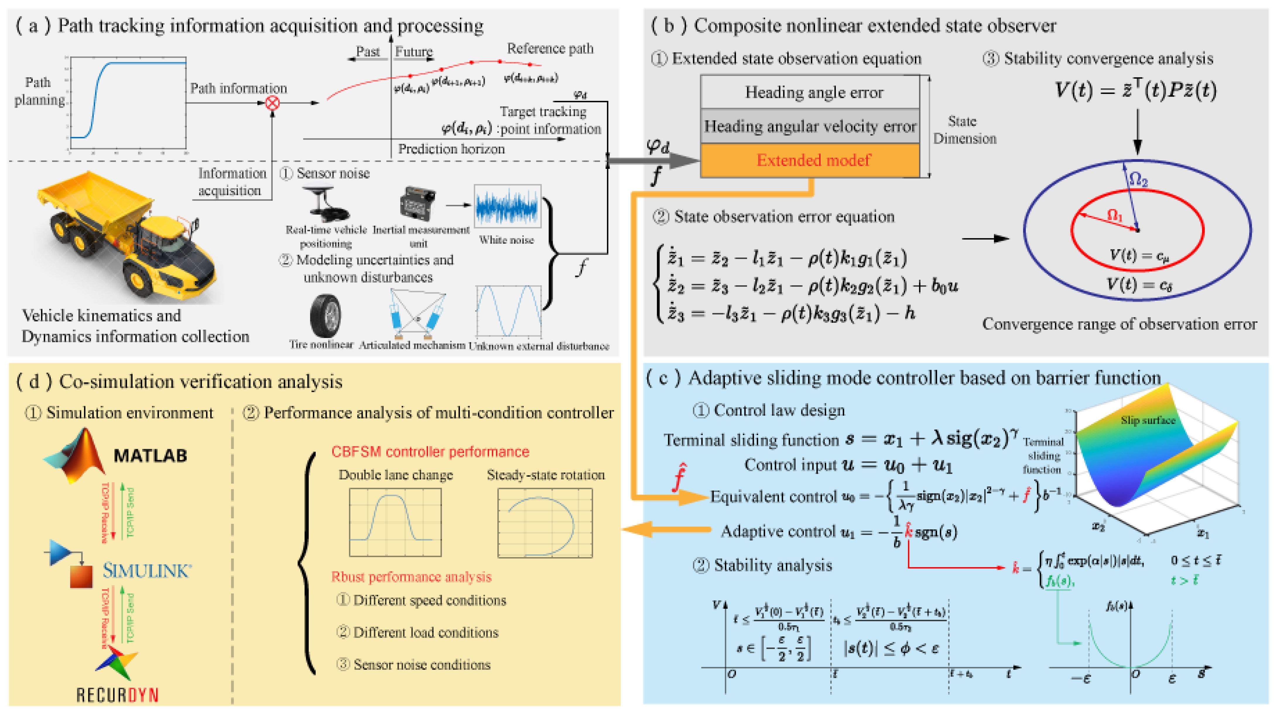
3. Composite Barrier Function Sliding Mode Control Based on an Extended State Observer

This section focuses on modeling uncertainties and unknown external disturbances in the path tracking control of articulated vehicles. The composite barrier function sliding mode control algorithm, based on composite nonlinear extended state observer (CNESO), is proposed. According to the comprehensive expected heading angle obtained above, combined with the articulated vehicle dynamics model, the path tracking control model can be derived. The CNESO is proposed to estimate the total disturbance of the system, which can suppress the peak overshoot phenomenon and observation noise problem of the traditional extended state observer (ESO). In this way, problems of observation overshoot and noise jitter are avoided, affecting effectiveness and robustness of the controller. Finally, combined with CNESO and the sliding mode controller based on barrier function, a composite barrier function sliding mode controller (CBFSMC) is proposed. Barrier function (BF) is used to design the adaptive control gain of the controller. Therefore, the robustness of the controller is enhanced, and control input chattering is suppressed.

3.1. Design and Performance Analysis of Composite Nonlinear Extended State Observer

3.1.1. Design of Disturbance Observer

Before designing the disturbance observer, extended state formulas for articulated vehicle path tracking control need to be derived. This chapter focuses on a dynamic model of an articulated vehicle, as represented by Formula (7). Through the above derivation and analysis, a path tracking control target is obtained as ${\phi }_{\mathrm{b}\mathrm{e}\mathrm{s}\mathrm{t}}$. To simplify the description of the control problem, ${\phi }_d$ will be used to represent ${\phi }_{\mathrm{b}\mathrm{e}\mathrm{s}\mathrm{t}}$ in the following text. The path tracking control system of an articulated vehicle is described as follows, and y represents system output.

$$\left\{\begin{array}{c}{\stackrel{·}{x}}_1=x_2=\stackrel{·}{\phi }-\stackrel{·}{{\phi }_d}\\ {\stackrel{·}{x}}_2=\stackrel{··}{\phi }-\stackrel{··}{{\phi }_d}\\ y=x_1\to 0\end{array}\right.$$

(20)

By combining Formulas (7) and (19), the path tracking control system for an articulated vehicle can be expressed as follows:

$$\begin{array}{c}{\stackrel{·}{x}}_1=x_2=\stackrel{·}{\phi }-\stackrel{·}{{\phi }_d}\\ {\stackrel{·}{x}}_2=\stackrel{··}{\phi }-\stackrel{··}{{\phi }_d}=a_{21}{v}_{y1}+a_{22}{w}_1+d\left(t\right)-\stackrel{··}{{\phi }_d}+bu\\ y=x_1\to 0\end{array}$$

(21)

In formula, $a_{21}$ and $a_{22}$ have the same parameters as in (7). $d_{\left(t\right)}$ represents the unmodeled dynamics of system and external disturbances, while $u=M$ denotes the control input of system.

Based on the above control formulas, $f=a_{21}{V}_{y1}+a_{22}{\omega }_1+\omega \left(t\right)-{\ddot{\phi }}_d$, f can be considered as the total lumped disturbance of the entire system. The path tracking control system for an articulated vehicle in Formula (21) can be rewritten as follows:

$$\left\{\begin{array}{c}{\stackrel{·}{x}}_1=x_2\\ {\stackrel{·}{x}}_2=f+bu\\ y=x_1\to 0\end{array}\right.$$

(22)

The total disturbance f is bounded and differentiable. It can be assumed that $h=\dot{f}$, and f is treated as a new state variable $x_3$. Formula (22) can be rewritten as follows:

$$\left\{\begin{array}{c}{\stackrel{·}{x}}_1=x_2\\ {\stackrel{·}{x}}_2=x_3+bu\\ {\stackrel{·}{x}}_3=h\\ y=x_1\end{array}\right.$$

(23)

Based on the above derivation and analysis, Formula (23) represents the expanded state formula for the path tracking control system of an articulated vehicle. Combined with the above derivation, the comprehensive expected heading angle is obtained. The complex path tracking control problem is simplified to a yaw angle tracking problem for the articulated vehicle. A disturbance observer and path tracking controller are designed based on Formula (23).

In this chapter, CNESO is proposed based on the idea of composite nonlinear control. In CNESO, observer gain can be adaptively adjusted according to observation error [18]. This achieves a non-switching combination of linear and nonlinear terms, which enables anti-noise and peak suppression.

$$\left\{\begin{array}{c}{\stackrel{·}{\widehat{z}}}_1={\stackrel{·}{\widehat{z}}}_2-l_1{\tilde{z}}_1-\rho \left(t\right)k_1{g}_1\left({\tilde{z}}_1\right)\\ {\stackrel{·}{\tilde{z}}}_2={\tilde{z}}_3-l_2{\tilde{z}}_1-\rho \left(t\right)k_2{g}_2\left({\tilde{z}}_1\right)+b_{0}u\\ {\stackrel{·}{\widehat{z}}}_3=-l_3{\tilde{z}}_1-\rho \left(t\right)k_3{g}_3\left({\tilde{z}}_1\right)\end{array}\right.$$

(24)

In the formula, $\widehat{z}={\left[{\widehat{z}}_1,{\widehat{z}}_2,{\widehat{z}}_3\right]}^T$ is the quantity of the observation state. $\tilde{z}={\widehat{z}}_1-x_1$ is the estimation error of $x_1$, while $l_i$ and $k_i$, i = 1, 2, 3 are the observation gain. $\rho \left(t\right)=e^{-\kappa \left|{\tilde{z}}_1\right|},\kappa >0; \rho \left(t\right)$ is an exponential function with observation error ${\tilde{z}}_1$ as the exponent and natural logarithm e as base [19]. ${g }_i\left({\tilde{z}}_1\right)=sign\left({\tilde{z}}_1\right){\left|{\tilde{z}}_1\right|}^{{\alpha }_i},0<{\alpha }_i<1$.

Combining Formulas (23) and (24), the estimation error of CNESO can be derived as follows:

$$\left\{\begin{array}{c}{\stackrel{·}{\tilde{z}}}_1={\tilde{z}}_2-l_1{\tilde{z}}_1-\rho \left(t\right)k_1{g}_1\left({\tilde{z}}_1\right)\\ {\stackrel{·}{\tilde{z}}}_2={\tilde{z}}_3-l_2{\tilde{z}}_1-\rho \left(t\right)k_2{g}_2\left({\tilde{z}}_1\right)+b_{0}u\\ {\stackrel{·}{\tilde{z}}}_3=-l_3{\tilde{z}}_1-\rho \left(t\right)k_3{g}_3\left({\tilde{z}}_1\right)-h\end{array}\right.$$

(25)

In formula, ${\tilde{z}}_i={\tilde{z}}_i-x_i$, i = 1, 2, 3. The form of the state space is as follows:

$$\stackrel{·}{\tilde{z}}=A\tilde{z}+Bh+G\left(t\right)$$

(26)

In the formula,

$$\left\{\begin{array}{c}A=\left[\begin{array}{ccc}-l_1& {\displaystyle \frac{1}{2}}& 0\\ -l_2& 0& {\displaystyle \frac{1}{2}}\\ -l_3& 0& 0\end{array}\right],B=\left[\begin{array}{c}0\\ 0\\ -1\end{array}\right]\\ G={\left[{\displaystyle \frac{1}{2}}{\tilde{z}}_2-\rho \left(t\right)k_1{g}_1\left({\tilde{z}}_1\right),{\displaystyle \frac{1}{2}}{\tilde{z}}_3-\rho \left(t\right)k_2{g}_2\left({\tilde{z}}_1\right),-\rho \left(t\right)k_3{g}_3\left({\tilde{z}}_1\right)\right]}^{{\rm T}}\end{array}\right.$$

(27)

Selecting an appropriate $l_i$ ensures that A is Hurwitz. Thus, there exist symmetrical positive define matrices P and Q satisfying $A^{T}P+PA=-Q$.

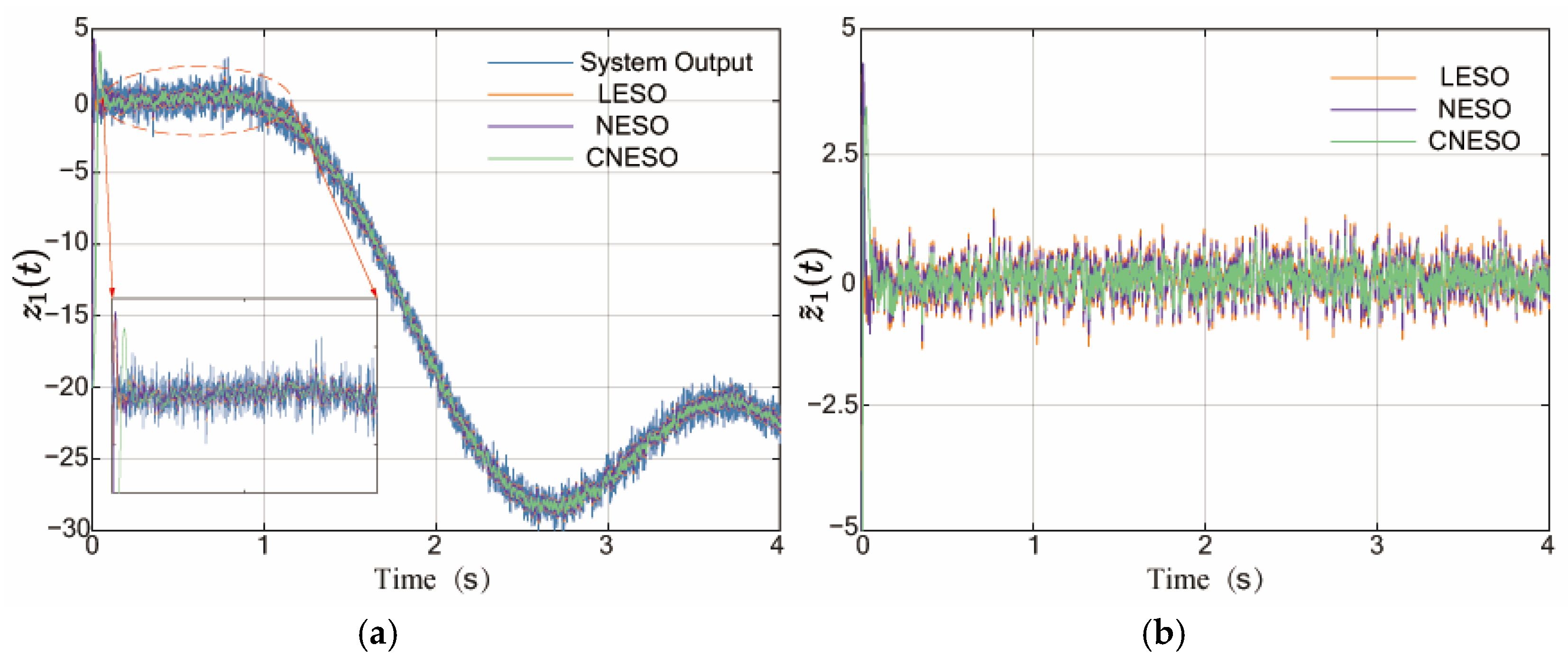
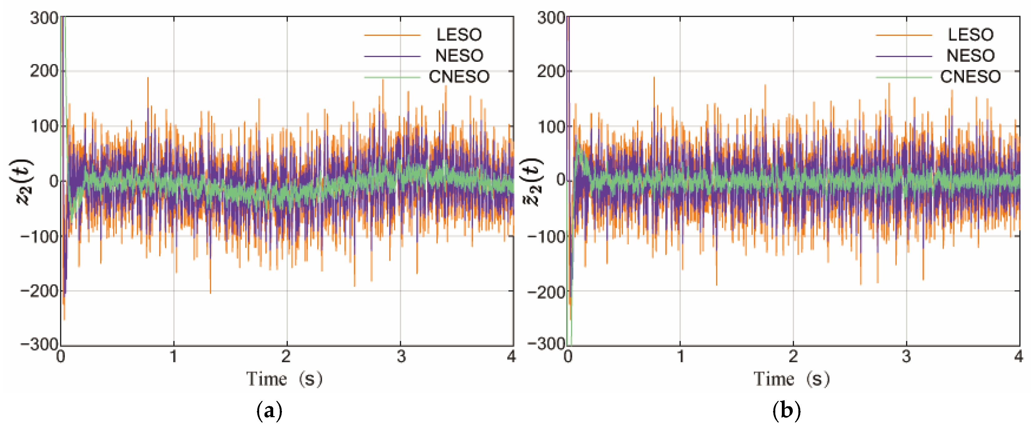
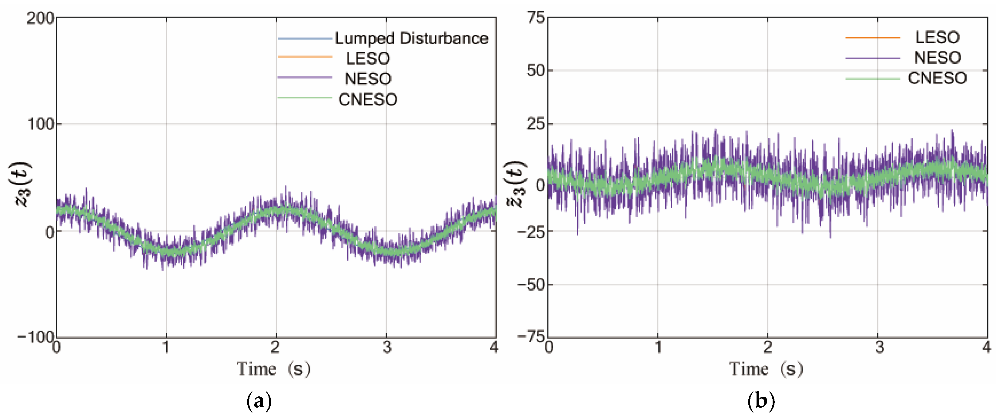
3.1.2. Analysis of Simulation Performance

In order to verify the anti-noise ability and peak suppression ability of CNESO, white noise (t) is added to the output y of the system (23). At the same time, a comparison of LESO, NESO, and CNESO is provided. The observation system is shown as follows:

$$\left\{\begin{array}{c}{\stackrel{·}{x}}_1=x_2\\ {\stackrel{·}{x}}_2=x_3+bu\\ {\stackrel{·}{x}}_3=h\\ y=x_1+\omega \left(t\right)\end{array}\right.$$

(28)

For Formula (28), the LESO form is designed as follows:

$$\begin{array}{c}{e}_1=z_1-y\\ {\stackrel{·}{z}}_1=z_2-l_1{e}_1\\ {\stackrel{·}{z}}_2=z_3-l_2{e}_1+bu\\ {\stackrel{·}{z}}_3=-l_3{e}_1\end{array}$$

(29)

In the formula, $e_1$ is estimation error. $z_1,z_2$ and $z_3$ are the quantity of the observation state. $z_1,z_2$ and $z_3$ are the estimates of $x_1,x_2$ and $x_3$, respectively. u and y are the input and output of system. $l_1,l_2$ and $l_3$ are the observer gain.

By selecting appropriate gain parameters, the observed value of LESO can converge to a true value. That is, $\underset{t\to \infty }{\lim }{z}_i=x_i$, i = 1, 2, 3. The main difference between NESO and LESO is that NESO uses the nonlinear function to estimate the system state. Common nonlinear functions include the following:

$$f_{al}\left(e,\alpha ,\delta \right)=\left\{\begin{array}{c}{\displaystyle \frac{e}{{\delta }^1-\alpha }}, \left|x\right|\le \delta \\ {\left|e\right|}^{\alpha }sign\left(e\right), \left|x\right|\ge \delta \end{array}\right.$$

(30)

In this paper, gain parameters of the observer are mainly determined by the bandwidth theorem. The value of the observer gain parameters $l_i$ and $k_i$ is obtained using the following formula: $l_1,k_1=3{\omega }_0,l_2,k_2=3{{\omega }_0}^2,l_3,k_3={{\omega }_0}^3$. Here, ${\omega }_0$ is the observer bandwidth. The detailed proof process and method for selecting observer bandwidth can be found in reference [20]. The bandwidth values in this paper are 50 and 40, respectively. To better analyze the performance of CNESO, the same parameters in all three observers are assigned the same values. Specific values are shown in

Table 1. Observation gain.

Observer	The Value of the Parameter
CNESO	$l_1=150$	$l_2=7500$	$l_3=\mathrm{12,500}$	$\kappa =0.4$
	$k_1=120$	$k_2=4800$	$k_3=\mathrm{64,000}$
	${\propto }_1=0.9$	${\propto }_1=0.8$	${\propto }_3=0.8$
LESO	$l_1=150$	$l_2=7500$	$l_3=\mathrm{12,500}$
NESO	$k_1=120$	$k_2=4800$	$k_3=\mathrm{64,000}$
	${\propto }_1=0.9$	${\propto }_1=0.8$	${\propto }_3=0.8$

.

The observation results of three observers for system output with white noise are shown in Figure 6. The convergence of all three observers is achieved in around 0.1 s. Moreover, CNESO can reduce the peak estimation errors effectively. Additionally, it can mitigate the impact of system output noise on observed states.

As shown in Figure 7, the observation effect of CNESO is better than LESO and NESO. The observed value of CNESO fluctuates less, while the other two observers change greatly. The error peak of CNESO is significantly smaller than the other two observers. The observation of three observers for unknown lumped disturbances is shown in Figure 8. The lumped disturbance estimation by NESO shows more significant fluctuations, while CNESO exhibits smaller fluctuations in its observation compared to LESO. Data in

Table 2. Statistical error of each estimated state.

Observation Status	Observer	Average Error	Maximum Error	Root Mean Square Error
$z_1$	LESO	0.649	1.414	0.806
	NESO	0.619	1.214	0.787
	CNESO	0.567	0.888	0.763
$z_2$	LESO	43.228	189.302	54.006
	NESO	30.791	133.372	38.528
	CNESO	9.239	38.672	11.554
$z_3$	LESO	4.826	21.614	6.027
	NESO	6.196	28.170	7.764
	CNESO	3.273	12.527	3.970

also show that CNESO has better observation performance in terms of mean error, maximum error and root mean square error of reaction deviation. Observation error is reduced by 15–80%. Among them, the average error of observed state $z_2$ was reduced by nearly 80%. In general, CNESO has good ability in peak suppression and noise filtering. Compared to LESO and NESO, CNESO shows significant improvement and exhibits more stable observation performance.

3.2. Design of Adaptive Sliding Mode Controller Based on Barrier Function

This section mainly introduces the design process of CBFSMC, which is used for the path tracking control of articulated vehicles. As mentioned in Section 2.2, the path tracking control problem is transformed into a heading angle tracking problem for articulated vehicles. CNESO is used to estimate the lumped disturbances of articulated vehicles. Error compensation technology is introduced to control and compensate for lumped disturbance. Furthermore, BF is used to design the adaptive control gain of a controller. BF adjusts control gain according to sliding variable s, ensuring that s remains in the predetermined region. And it can effectively reduce control chattering without affecting additional convergence time.

Based on Formulas (7) and (19), the path tracking control system of an articulated vehicle can be expressed as follows:

$$\left\{\begin{array}{c}{\stackrel{·}{x}}_1=x_2\\ {\stackrel{·}{x}}_2=f+bu\\ y=x_1\to 0\end{array}\right.$$

(31)

To ensure the rapid convergence of the tracking error and effectively avoid singularity issues, the nonsingular terminal sliding function s is introduced [21] as follows:

$$s=x_1+\lambda \mathrm{sig}{\left(x_2\right)}^{\gamma }$$

(32)

In the formula, control parameter λ > 0; 1 < γ < 2 needs to be designed, and the sign function ${\mathrm{s}\mathrm{i}\mathrm{g}\left(x\right)}^a$ represents the following simplified expression:

$$\mathrm{sig}{\left(x\right)}^a={\left|x\right|}^a\mathrm{sgn}\left(x\right)$$

(33)

where $\mathrm{s}\mathrm{g}\mathrm{n}\left(·\right)$ is the standard sign function [22].

To achieve yaw angle tracking, the control law is designed as follows:

$$u=u_0+u_1$$

(34)

In the formula, $u_0$ is the equivalent control term; $u_1$ is an adaptive control term.

The differential of s can be obtained by the following formula:

$$\begin{array}{ll}\stackrel{·}{s}& ={\stackrel{·}{x}}_1+\lambda \gamma {\left|x_2\right|}^{\gamma -1}{\stackrel{·}{x}}_2\\ & =x_2+\lambda \gamma {\left|x_2\right|}^{\gamma -1}\left(\widehat{f}+bu\right)\end{array}$$

(35)

In the formula, $\widehat{f}$ is estimated by CNESO in the previous section.

Let $\dot{s}=0$; then, the equivalent control term is obtained as follows:

$$u_0=-\left\{{\displaystyle \frac{1}{\lambda \gamma }}sign\left(x_2\right){\left|x_2\right|}^{2-\gamma }+\widehat{f}\right\}{b}^{-1}$$

(36)

In addition, the adaptive control term is designed as follows.

$$u_1=-{\displaystyle \frac{1}{b}}\widehat{k}\mathrm{sgn}\left(s\right)$$

(37)

In the formula, $\widehat{k}$ represents the adaptive control gain to be designed.

Constant c is defined to represent the region boundary of the final convergence of the tracking error. In addition, $\overline{t}$ is defined as the time when s first arrives at region $\left[– {\displaystyle \frac{\epsilon }{2}}, {\displaystyle \frac{\epsilon }{2}} \right]$ from any initial value outside the region. That is, a = b. Otherwise, $\left|s\left(0\right)\right|\le {\displaystyle \frac{\epsilon }{2}},\overline{t}=0$. The adaptive law of control gain $\widehat{k}$ is as follows:

$$\widehat{k}=\left\{\begin{array}{c}\eta {\displaystyle {\int }_0^t\exp \left(\alpha \left|s\right|\right)\left|s\right|dt,} 0\le t\le \overline{t}\\ f_b\left(s\right), \mathrm{t}>\overline{t}\end{array}\right.$$

(38)

In the formula, control parameter $\alpha \ge 0$, $\eta >0$. And the initial value of $\widehat{k}$ is $\widehat{k}\left(0\right)\ge 0$. $f_b\left(s\right)$ is the barrier function in the following form:

$$f_b\left(s\right)={\displaystyle \frac{\left|s\right|}{\epsilon -\left|s\right|}},s\in \left(-\epsilon ,\epsilon \right)$$

(39)

Analysis (38) shows that the exponential term $\mathrm{e}\mathrm{x}\mathrm{p}\left(\alpha \left|s\right|\right)$ in the formula can make the sliding variable converge to $\left[– {\displaystyle \frac{\epsilon }{2}}, {\displaystyle \frac{\epsilon }{2}} \right]$ at a faster convergence rate, that is, the smaller $\overline{t}$. When the sliding variable s is far away from the origin, a faster convergence effect can be obtained [23]. There is variation in adaptive control gain $\widehat{k}$ with respect to the sliding variable when $t>\overline{t}$. When $\left|s\right|$ increases in the range of (0, ε), $f_b\left(s\right)$ tends to infinity. Therefore, adaptive control gain $\widehat{k}$ is significantly improved. Adaptive control term $u_1$ in the control input is increased according to Formula (37). As a result, sliding variable s is quickly brought back to the origin. On the other hand, once $\left|s\right|$ decreases, $\widehat{k}$ will also decrease accordingly. Therefore, excessive control input can be avoided. The stability and performance analysis process of the CBFSMC controller are shown in Appendix A.

3.3. Verification Analysis of Joint Simulation

This chapter mainly focuses on building a MATLAB/Simulink-RecurDyn co-simulation environment to validate the performance of the CBFSMC path tracking controller. CBFSMC is implemented in MATLAB/Simulink by S-functions. RecurDyn V9R2 is a multi-body dynamics simulation software. RecurDyn can simulate various real-world motions in a virtual environment. Reference points of path planning are quickly searched by upper computer using KD-Tree. Additionally, communication with MATLAB is established via TCP/IP, forming a closed control loop. In Recurdyn, communication interface for co-simulation with Simulink is defined. This includes wheel speed and control input torque, as well as position, attitude, and the longitudinal velocity and yaw velocity of the vehicle.

3.3.1. Comparative Analysis of CBFSMC Controller Performance

In order to verify the proposed CBFSMC path tracking controller, Nonsingular Terminal Sliding Mode [24,25,26,27] (NTSM) and Active Disturbance Rejection Control [18,28,29] (ADRC) are adopted, respectively. At the same time, typical working conditions, such as double lane change and steady-state rotation, are set up to verify the performance of the controller.

In order to verify the control performance of CBFSMC, NTSM and ADRC are used as comparison controllers. The control law of NTSM is designed as follows, where $k_1, k_2$ are adjustable parameters.

$$u=-\left\{{\displaystyle \frac{1}{\lambda \eta }}sign\left(x_2\right)\left|x_2\right|{\left|x_2\right|}^{2-\eta }+f+k_{1}s+k_2\tanh \left(s\right)\right\}{b}^{-1}$$

(40)

The control law of ADRC is designed as follows:

$$u=-{\displaystyle \frac{fhan\left(z_1,c{z}_2,r,h_1\right)+z_3}{b}}$$

(41)

In the formula, $h_1$ is the sampling interval; r is an adjustable parameter. $fhan=-r_0\left({\displaystyle \frac{a}{d}}-sign\left(a\right)\right)s_a-r_{0}sign\left(a\right)$. For specific parameter definitions, readers are referred to Reference [18].

In engineering practice, factors such as measurement noise, control signal chattering, and limited control force will affect system performance. The qualitative selection criteria of controller parameters in this experiment are introduced. Parameters $\lambda$ and $\gamma$ dominate the dynamic characteristics of sliding mode function $s$, as shown in Formula (32). Smaller $\gamma$ or larger $\gamma$ can accelerate the convergence rate of tracking error e. However, according to the derivation of Formula (36), this will lead to an increase in control input or an increase in chattering. Here, we finally choose $\lambda =0.053,\gamma =1.4$. Parameter $\epsilon$ defines expected the boundary of the tracking error. In addition, parameter $\epsilon$ is the key performance index of the positioning system. In this experiment, $\epsilon =0.05$ is chosen to improve tracking accuracy and robustness. Based on adaptive law (38), the control gain needs to be greater than the upper bound of disturbance at the initial time. When initial sliding mode variable $s\left(0\right)$ significantly deviates from zero, a larger exponential parameter $\alpha$ effectively enhances the adaptation rate. When $s\left(0\right)$ is close to zero, increasing $\eta$ achieves a proportional rate improvement. In this study, $\eta =1.5,\alpha =2$ is ultimately adopted. In order to compare the control performance of different controllers, the same parameters value are used for CBFSMC and NTSM. Specific parameters of other controllers are shown in

Table 3. Gain of different controllers.

Controller	The Value of the Parameter
CBFSMC	$\lambda =0.053$	$\eta =1.5$	$\alpha =2.27$	$\epsilon =0.05$
NTSM	$\lambda =0.053$	$\eta =1.5$	$k_1=50$	$k_2=0.5$
ADRC	$c=5$	$r=5$	$h_1=0.001$

.

• Working condition of double lane change

To verify the lateral motion control performance of the CBFSMC in path tracking, the working conditions of typical double lane change are used. And the initial lateral error is set to 2 m. The control performance of the CBFSMC controller is compared with that of NTSM and ADRC controllers. In order to facilitate the analysis of simulation results, the simulation conditions of the three controllers are the same. Moreover, the simulation time is 40 s. The results of path tracking simulation and error analysis are shown in Figure 9.

Figure 9a and

Table 4. Error of different controllers in double lane change condition.

Controller	Convergence Time (s)	Average Error (m)	Steady-State Maximum Error (m)
ADRC	9.53	0.313	0.652
NTSM	6.38	0.322	0.692
CBFSMC	5.58	0.202	0.215

show double lane change in the path tracking results of three controllers for comparison. The convergence speed of the initial lateral error for CBFSMC is superior to that of NTSM and ADRC. The convergence time of CBFSMC is 5.58 s, which is 41.4% and 12.5% shorter compared to ADRC and NTSM, respectively. The steady-state error of the vehicle during driving is also smaller than that of NTSM and ADRC. The maximum steady-state error of CBFSMC is 0.215 m, which is reduced by 66.9% and 68.9%, respectively, compared with ADRC and NTSM. The average error of CBFSMC is 0.202 m, which is reduced by 35.5% and 38.3%, respectively, compared with ADRC and NTSM. The above error analysis shows that the control performance of CBFSMC is better than NTSM and ADRC. Moreover, as shown in Figure 9b, lateral error comparison indicates that all three controllers exhibit an increase in error at $t=15 \mathrm{s}$ and $t=35 \mathrm{s}$. This phenomenon is caused by the preview distance when the vehicle is turning. A comparison of the control inputs in Figure 9c shows that the ADRC controller exhibits significant oscillations. Compared with the control input of the three controllers in Figure 9c, the ADRC controller has significant chattering. ADRC uses high-gain nonlinear functions to achieve stable control. Therefore, frequent switching of the nonlinear function results in control input chattering. The NTSM controller exhibits significant control input chattering during straight-line driving. However, the control input is stable when steering. During the steering of the vehicle, disturbance such as tire nonlinearity increases. Therefore, a consistent switching coefficient of NTSM cannot estimate disturbance value. A phenomenon whereby the sliding surface is lost and error increases is produced. When a vehicle runs smoothly within 17–18 s, disturbance is reduced. NTSM returns to the sliding mode surface while generating control input chattering. CBFSMC effectively resolves the above issue by employing an adaptive control gain. Adaptive gain is adjusted by BF based on the sliding variable. Thus, the control chattering caused by the frequent switching of the sliding variable is avoided. The control performance is obviously better than NTSM and ADRC. As shown in Figure 9d, CBFSMC can quickly converge towards the reference path, even in the presence of initial lateral errors. When the lateral error converges to a small value, the yaw angle error of path tracking remains within a narrow range. Based on the above results and theoretical analysis, the control performance of CBFSMC is superior to that of NTSM and ADRC. Additionally, the control input of CBFSMC is relatively smooth.

2.

Work condition of steady-state rotation

To verify the steering tracking performance of CBFSMC, the typical steady-state rotation condition is set. The initial lateral error is set to 2 m. Simulation conditions for three controllers are the same, with a simulation time of 28 s. The simulation results are shown in Figure 10.

In Figure 10, the convergence speed of CBFSMC is better than that of NTSM and ADRC. And the steady-state error is better than NTSM and ADRC. As shown in

Table 5. Error of different controllers in steady-state rotation condition.

Controller	Convergence Time (s)	Average Error (m)	Steady-State Maximum Error (m)
ADRC	9.26	0.317	0.052
NTSM	7.73	0.324	0.067
CBFSMC	5.57	0.261	0.011

, the convergence time for CBFSMC from the initial error is 5.57 s, which is reduced by 39.4% and 27.9% compared to ADRC and NTSM. The average error is 0.261 m, which is reduced by 17.1% and 19.4%, respectively, compared with ADRC and NTSM. The maximum steady-state error is 0.011 m, which is reduced by 78.8% and 83.6%, respectively, compared with ADRC and NTSM. Based on an analysis of the above error results, the steering tracking performance of the CBFSMC controller is superior to that of NTSM and ADRC. CBFSMC can effectively control a vehicle to perform steady-state rotation. As shown in Figure 10c, when the error approaches the target, CBFSMC employs an adaptive control gain. During a stable tracking process with smaller errors, sliding variable s becomes smaller, resulting in the switching term gain being reduced. As a result, control input chatter can be effectively suppressed. As shown in Figure 10d, CBFSMC is able to rapidly converge to the reference path, even with an initial lateral error. Moreover, the lateral error converges to a small value, while the yaw angle error in path tracking remains within a narrow range.

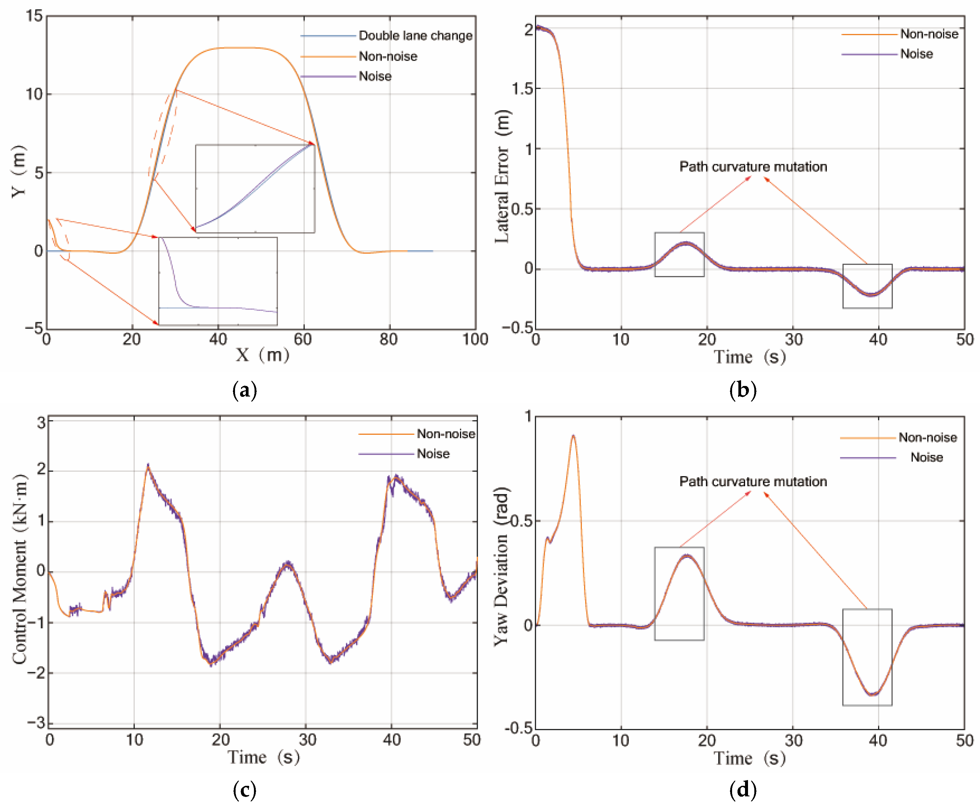
3.3.2. Robust Performance Analysis of CBFSMC Controller

Articulated vehicles in engineering operations typically work under varying conditions, including different speeds and loads. This is usually accompanied by load changes, road disturbance excitation caused by an unstructured environment and the dynamic nonlinear characteristics of articulated wheeled vehicles. Uncertainty in vehicle dynamics parameters presents challenges in controller design. The CBFSMC controller combines CNESO to estimate the lumped disturbances of a vehicle. The drawback of traditional controllers, which require precise dynamic parameters, is avoided. Additionally, it maintains stable controller performance with excellent robustness. In order to verify the robust performance of CBFSMC, different working conditions such as different vehicle speeds, different loads and sensor noise are designed. A comprehensive analysis is conducted to verify the robustness of CBFSMC under various conditions.

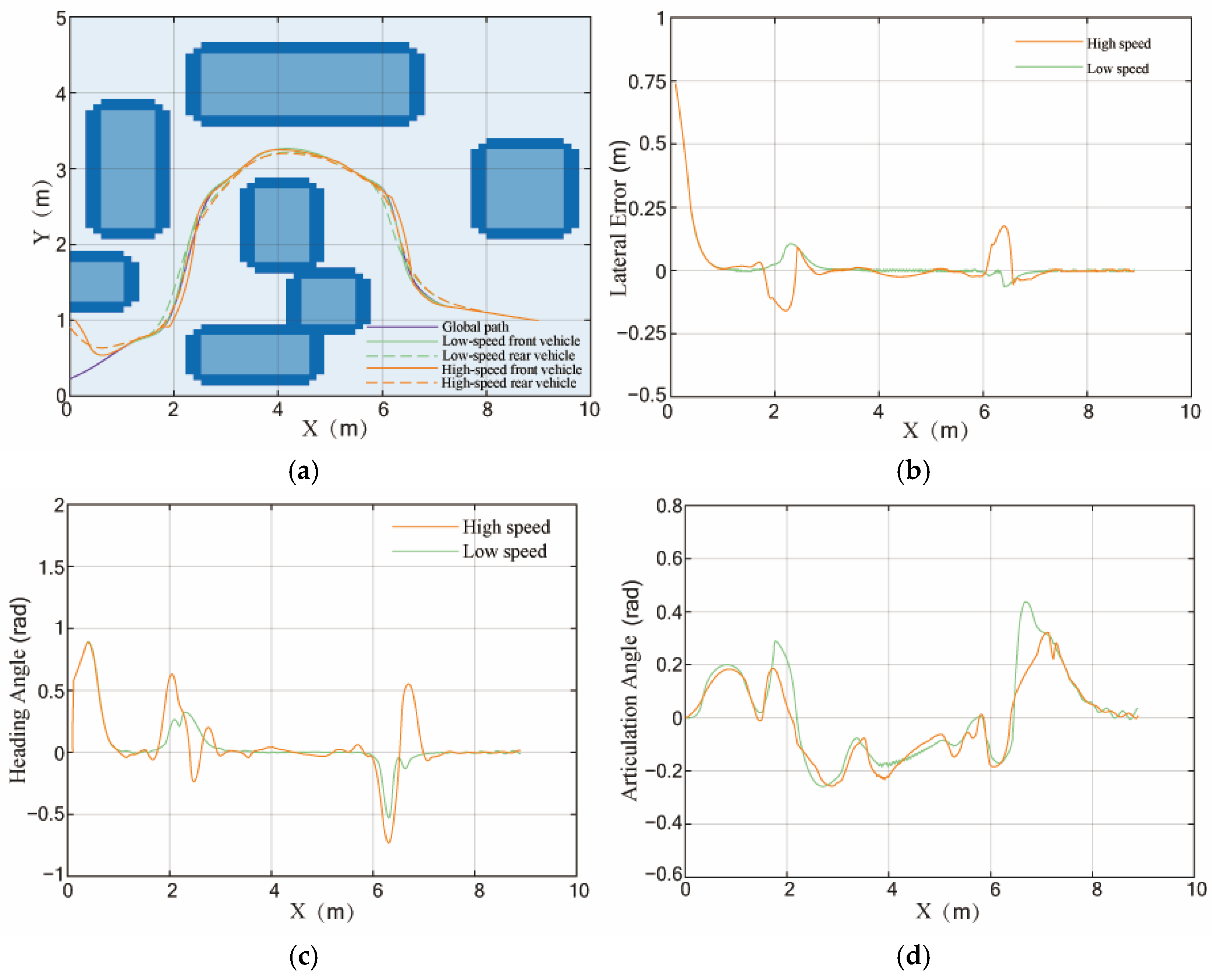
• Work condition of different speeds

Different from the traditional controller, CBFSMC does not need to set different control parameters for different operating speeds. CBFSMC exhibits strong robustness to changes in vehicle speed. This is primarily because CBFSMC can dynamically estimate and compensate for total disturbances in the system. In this subsection, different operating speeds for articulated vehicles are set under double lane change conditions. Vehicle operating speeds are set as follows: v = 2 m/s, v = 4 m/s, and v = 6 m/s. The simulation results are shown in Figure 11.

By comparing Figure 11a and Figure 11b, it can be seen that CBFSMC can control articulated vehicles to achieve double lane change path tracking control under different vehicle speed conditions with an initial lateral error of 2 m. Moreover, the tracking performance remains consistent across different vehicle speeds. The lumped disturbances of vehicles under different conditions are estimated by CNESO in the CBFSMC controller. And the control input compensates for disturbances. This ensures that the controller exhibits good robustness to different speeds. Initial lateral errors for all three speed conditions converge within a 5 m running distance. The lateral steady-state error is maintained around 0.25 m for all speed conditions. At the same time, the lower the speed, the higher the path tracking accuracy of vehicles. With increased vehicle speed, the tires of a vehicle may enter the nonlinear region when the vehicle turns at a large angle. Therefore, the vehicle model experiences significant errors. As shown in Figure 11c, the control torque is always confined within a certain range, satisfying actuator constraints. As shown in Figure 11d, the steady-state error of yaw angle remains within the same range. Stable path tracking control at different vehicle speeds can be achieved. Based on the above simulation analysis, the proposed CBFSMC controller has certain robustness to vehicle speed. Simultaneously, stable and accurate path tracking control can be achieved.

2.

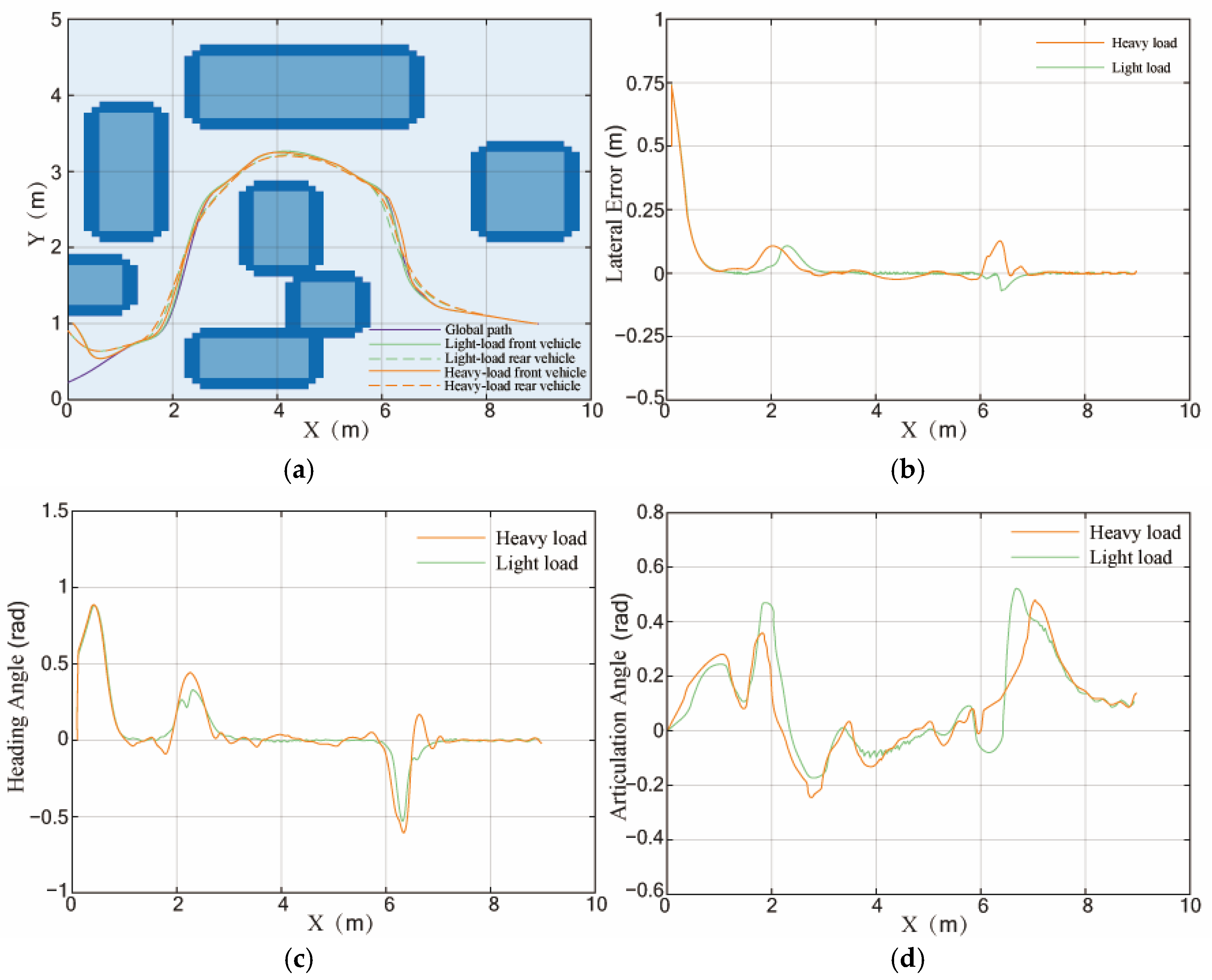
Work condition of different loads

In this section, combined with the double lane change path, different load conditions of articulated vehicles are set. The main conditions are divided into three: light load, medium load, and heavy load. This mainly simulates operating environments with variable loads during the operation of articulated vehicles.

The simulation results are shown in Figure 12. Comparing the lateral errors in Figure 12a,b, lateral error trends are similar across different load conditions. The initial lateral displacement errors of three load conditions can quickly converge to near zero. At the same time, the convergence speed is faster and tracking accuracy is higher for lighter loads. Conversely, for heavier loads, the convergence speed is slower and tracking accuracy is lower. This is due to the larger steering torque required in heavier load conditions, leading to a longer response time. As a result, control performance is affected. As shown in Figure 12c, the steering torque required for lighter loads is smaller, while the torque required for heavier loads is larger. Due to the limitations of control inputs, control inputs are constrained within a specific range to comply with actuator limitations. As shown in Figure 12d, the steady-state error of yaw angle for all three load conditions remains within a similar range. The yaw angle error under heavy load conditions requires a longer convergence time. This is related to the larger control input and longer control time required. However, convergence can be achieved within a relatively short amount of time. Based on the above simulation analysis, the proposed CBFSMC controller has certain robustness to vehicle load. Simultaneously, stable and accurate path tracking control can be achieved.

3.

Work condition of sensor noise

Sensor error involves many aspects such as manufacturing, environment, installation and use. Noise, deviation, drift and cross-axis sensitivity are also caused by it. Due to the influence of electronic noise, mechanical vibration and other factors, in practical engineering applications, sensor noise can have a significant impact on control performance. In path tracking control, the yaw angle is typically measured by an Inertial Measurement Unit (IMU) installed on a vehicle. However, sensor data often contain Gaussian-distributed white noise, with a signal-to-noise ratio (SNR) typically around 40 dB. Therefore, in this section, noise is added to the yaw rate. The impact of sensor noise on the performance of the control algorithm is analyzed.

Figure 13 shows that an articulated vehicle follows the reference path accurately under the CBFSMC controller. As shown in Figure 13c, sensor noise increases the chattering of the control input. At the same time, the phenomenon of local chattering is intensified. However, overall chattering remains within the executable range. In general, as shown in Figure 13a,b,d, CBFSMC can still stably control articulated vehicle path tracking control, despite the influence of sensor noise. Based on the above analysis, the system still has a stable and accurate path tracking performance when the system has measurement noise. The CBFSMC controller demonstrates strong robustness to noise.

4. Experimental Validation

This section aims to verify the path tracking method proposed in this paper, which is composite barrier function sliding mode control based on an extended state observer. This paper takes into account the articulated vehicle structure, considering both site limitations and safety issues during debugging. A test prototype vehicle is constructed to meet the experimental requirements. The prototype vehicle is used to verify the proposed path tracking control method for unmanned articulated vehicles.

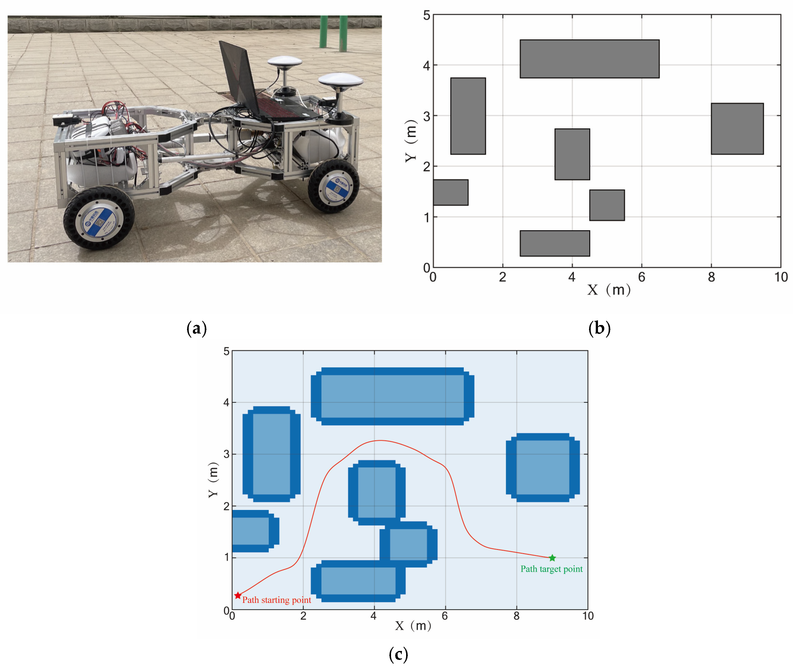
4.1. Introduction to Prototype Platform of Unmanned Articulated Vehicle

The overall design of the prototype test platform for articulated vehicles is shown in Figure 14. The upper-level control software adopts a hierarchical control framework. Data are first received and preprocessed by STM32, and then sent to ROS for tracking control calculation. Part of the tracking control software is implemented on the ROS. The prototype primarily consists of a data acquisition system, communication control system, and execution system. It is mainly responsible for state acquisition and processing, the calculation of path tracking control quantity and control execution action. Its purpose is to form a path tracking control closed loop and complete the path tracking control of articulated vehicles.

The data acquisition system is mainly divided into vehicle positioning information acquisition and state information acquisition. The data acquisition system is mainly composed of real-time kinematic (RTK), a cable displacement sensor, a tension and pressure sensor, IMU, a GCAN data acquisition instrument and a hub motor integrated encoder. The communication control system mainly includes a computer, STM32, Kvaser Leaf Light, a hub motor controller, and a servo electric cylinder controller. The execution system mainly includes a hub motor and servo electric cylinder. The control signal is transmitted to the computer through the Kvaser Leaf Light and the computer is used as the controller. The characteristics of CAN signal bus transmission in Kvaser Leaf Light are used by the control signal. Thus, signal and communication connections between each component are established. Ultimately, the drive control of the vehicle wheel motor and the motion control of articulated steering, as well as remote control signal transmission, sensor signal acquisition and transmission, computer software monitoring and other functions, are achieved.

4.2. Experimental Verification of Path Tracking Method

In order to verify the performance of the global path planning algorithm and robust tracking controller for articulated vehicles proposed in this paper, a global path tracking test is carried out based on the prototype. Considering site setup and the safety of test personnel and vehicles, a 10 m × 5 m open test area is selected. Virtual obstacles are set, and the global reference path is obtained by the global path planning algorithm. In addition, different operating conditions are set to verify the path planning and tracking algorithm proposed in this paper. The prototype and virtual test field are shown in Figure 15a,b. In order to verify the lateral error control ability of the path tracking controller, the initial offset of the current vehicle position is set to 0.75 m. Data transformation is performed based on set starting and target points, along with current vehicle position measured by RTK. The planned path is shown in Figure 15c. As shown in Figure 15c, based on starting and target point information, the planned path does not collide with the obstacle. Additionally, the path, optimized by a Voronoi diagram and Euclidean distance field map, is distributed in an open environment. The path is generally far from obstacles, ensuring vehicles can operate safely. The path is smooth and without any sudden curvature changes, ensuring stable and safe vehicle operation.

A global path is obtained through the planning algorithm. Various operating conditions are set to validate the performance of the path tracking controller, including different vehicle speeds, load conditions, and other working conditions. The test results are as follows.

4.2.1. Path Tracking Test Under Different Speed Conditions

In order to analyze and validate the robustness of the path tracking controller under different vehicle speed conditions, two different speeds are set based on the maximum speed of prototype vehicle. The high speed is set to 2 m/s, and the low speed is set to 0.5 m/s. Dynamic parameters such as the lateral error and heading angle error of the front vehicle body under two working conditions are compared, respectively. Current vehicle data can be obtained in real-time through RTK. The position of vehicle and heading angle information can be obtained through data transformation. The path tracking results are shown in Figure 16.

The global path tracking test results under set speed conditions are shown in Figure 14. Under different speed conditions, the front and rear vehicles of prototype vehicle do not collide with the obstacle. All vehicles followed the reference path effectively. The lateral error convergence is shown in Figure 16b. The initial lateral error of 0.75 m is present at the starting position. Since vehicles are in the initial acceleration phase, the speed difference is relatively small. Both speed conditions tracked the reference path within 1 m. When x = 2 m, the prototype vehicle follows the reference path to turn left. The lateral error is larger during high-speed operation compared to low-speed operation. This is mainly due to the higher speed, which caused the vehicle to deviate to the right from reference path. However, deviation quickly converges to within 0.1 m. When x = 6 m, the prototype vehicle follows the reference path to turn right. During the steering process, the maximum lateral error remains within 0.25 m. The maximum lateral error of the high-speed condition is 0.2 m, while the maximum lateral error of the low-speed condition is within 0.1 m. Moreover, in both speed conditions, the vehicle position is adjusted within 1 m to achieve lateral error convergence. Based on the above analysis, the path tracking controller proposed in this paper can adapt to different vehicle speed conditions.

The heading angle error and articulated angle variation results for path tracking under different vehicle speed conditions are shown in Figure 16c,d. The heading angle error is the difference between the current heading angle of the front vehicle body of the prototype and the calculated combined expected heading angle. The initial position and starting heading angle are same for both vehicle speed tracking tests. Moreover, the initial speed difference is relatively small. The initial heading angle errors are similar, and the convergence rates are close. The initial heading angle error is eliminated within 1 m by the prototype vehicle. When turning at x = 2 m and x = 4 m, the heading angle error of the vehicle changes greatly under high-speed conditions. The maximum heading angle error is 0.6 rad. This indicates that there is a significant difference between the current heading angle of the front vehicle body and the comprehensive expected heading angle. At higher speeds, the generation of lateral error leads to changes in the comprehensive expected heading angle. This indicates that, at higher speeds, the lateral error is quickly corrected by the path tracking controller. At the same time, the heading angle of the front vehicle body can be adjusted to achieve better tracking of the reference path. During the path tracking process, the change in vehicle articulated angle remains within the articulated angle constraints. Moreover, no extreme situations with abrupt changes in articulated angle occurred. In conclusion, the path tracking controller proposed in this paper is able to smoothly track the reference path under different vehicle speed conditions. And the path tracking performance is stable and consistent. Reference path tracking can be achieved at different vehicle speeds. Therefore, the path tracking controller proposed in this paper demonstrates strong robustness under different vehicle speed conditions.

4.2.2. Path Tracking Tests Under Different Load Conditions

In order to verify the robust performance of the path tracking controller for different load conditions, two different load conditions are set compared to the mass of the prototype itself. The two load conditions are set as light load (m = 10 kg) and heavy load (m = 30 kg). The lateral error, heading angle error, and other dynamic parameters of the front vehicle body are compared for two load conditions. The initial vehicle position and heading angle are obtained in real-time by RTK and then converted accordingly. The path tracking results under different load conditions are shown in Figure 17.

The tracking path of the front and rear vehicles and the lateral error of the front vehicle under different load conditions are shown in Figure 17a,b. The driving paths of the vehicle under two load conditions are distributed in the lateral local neighborhood of the global path. Additionally, neither the front nor rear vehicle body collided with any obstacles. The security of the global path is verified by this phenomenon. As shown in Figure 17b, the initial lateral error of the vehicle under two load conditions converges within 1 m. During the turning process at x = 2 m and x = 6 m, the maximum lateral error under the heavy-load condition is 0.13 m, while the maximum lateral error under the light-load condition is 0.1 m. In both cases, the lateral error remained within 0.2 m. Therefore, a vehicle can follow the global path under different load conditions. The above analysis shows that the global path is successfully followed under different load conditions by the path tracking controller proposed in this paper.

The heading angle error of the front vehicle body and the articulation angle variation under different load conditions are shown in Figure 17c,d. The heading angle errors of the two load conditions change from an initial 0 rad to approximately 0.8 rad. This is mainly a change in comprehensive expected heading angle caused by the initial lateral error. Steady change in the vehicle heading angle leads to change in the heading angle error. Around x = 1m, the heading angle error of the vehicle converges to 0. The vehicle begins to turn at x = 2 m and x = 6 m. Due to the consideration of actuator constraints and driving stability, the heading angle of the front vehicle body does not change rapidly. Therefore, the heading angle error is generated. Under the heavy-load condition, the maximum heading angle error is 0.47 rad and −0.6 rad. Under the light-load condition, the maximum heading angle error is 0.35 rad and −0.5 rad. However, in both cases, the heading angle errors converge to 0 relatively quickly. This demonstrates that the controller can effectively track the reference path and maintain the desired heading angle. This demonstrates that the controller can track the heading reference value of the reference path well. The articulation angle changes smoothly and steadily, without any sudden or extreme fluctuations. Based on an analysis of the above test results, the path tracking controller proposed in this paper can handle changes in dynamic parameters under different load conditions. And the tracking performance is relatively consistent. Path tracking control for articulated vehicles under different loading conditions can be achieved. Therefore, the path tracking controller proposed in this paper can achieve robust and precise path tracking control under different loading conditions. In addition, it demonstrates strong robustness under different loading conditions.

5. Discussion

The target of research methodology in this paper primarily focuses on articulated vehicles in mining transportation machinery. This method is verified to be feasible. In the field of ground unmanned vehicles, there are other advanced control methods available, for example deep learning control and model-free adaptive control, which have shown excellent performance in similar applications. A comparative study is conducted from both theoretical and experimental perspectives. It demonstrates that the CBFSMC method is currently more suitable for the research work in our present scenario.

In theoretical comparison, the advantage of deep learning-based control methods lies in their ability to directly learn the dynamic characteristics of complex systems through neural networks. These methods are particularly suitable for high-dimensional nonlinear problems, such as lane-keeping and autonomous vehicle path tracking. However, deep learning-based control methods require a large amount of training data, and their real-time performance may be limited. Model-free adaptive control does not need a system model, and parameters can be adjusted online by the dynamic linearization technique. It is suitable for model-uncertain or time-varying systems. However, the robustness of model-free adaptive control may be limited by the accuracy of disturbance estimation. The CBFSMC method achieves a relative balance between model dependence and real-time performance. It reduces model dependence based on fuzzy logic and ensures the strong robustness of sliding mode control.

In terms of experimental comparison, limited by the experimental conditions, current research focuses on improving traditional control methods. In follow-up work, we will collect and apply driverless data from real vehicles in related enterprises. We also extend and compare the control effects of CBFSMC with a deep learning-based controller and model-free adaptive control. Future research directions we will take include, for example, overshoot, convergence speed, and robustness index.

The CBFSMC method becomes more and more complex with the system. The real-time implementation of the CBFSMC method on a resource-constrained platform may face challenges. However, the current hardware platform (an industrial computer equipped with an Intel i7-8700T CPU) has shown sufficient computational power to achieve real-time operation (with an update frequency greater than 200 Hz). Additionally, the feasibility of this control method has been demonstrated. The further optimization of resource-constrained systems will be pursued in our ongoing industrial cooperation projects. Considering computational complexity, future work will focus on how to optimize the algorithm to reduce computational burden. At the same time, directions for maintaining control performance are studied.

6. Conclusions

A composite barrier function sliding mode control method based on a extended state observer for the path tracking of unmanned articulated vehicles is proposed in this paper. Aiming at modeling uncertainties and unknown external disturbances, a composite nonlinear extended state observer is designed to estimate lumped disturbances and state variables, and the estimated values of lumped disturbances are introduced into the path tracking control model using error compensation technology. In addition, an adaptive composite barrier function sliding mode controller is designed to achieve path tracking control.

During the co-simulation verification analysis, a composite nonlinear extended state observer exhibits good peak overshoot and observation noise suppression effects. We verified that CBFSMC has a better control performance and lower control input chattering. The prototype vehicle experimental results demonstrate that the path tracking control method for unmanned articulated wheeled vehicles proposed in this paper can meet operational requirements under different working conditions. Moreover, robust and precise path tracking control is achieved.

In the future, this study will hold significant reference value for enhancing the intelligence of engineering vehicles and improving work efficiency in construction projects.

References

1. Hung, N.; Rego, F.; Quintas, J.; Cruz, J.; Jacinto, M.; Souto, D.; Potes, A.; Sebastiao, L.; Pascoal, A. A review of path following control strategies for autonomous robotic vehicles: Theory, simulations, and experiments. J. Field Robot. 2023, 40, 747–779. [Google Scholar] [CrossRef]
2. Gu, X. Research on Path Planning and Path Tracking Control Methods for Articulated Wheeled Operating Vehicles. Master’s Thesis, Jilin University, Changchun, China, 2024. [Google Scholar]
3. Liao, K.; Liou, J.; Hidayat, M.; Wen, H.-T.; Wu, H.-Y. Detection and Analysis of Aircraft Composite Material Structures Using UAV. Inventions 2024, 9, 47. [Google Scholar] [CrossRef]
4. Meng, Q.; Gao, L.; Xie, H.; Dou, F. Analysis of the Dynamic Modeling Method of Articulated Vehicles. J. Eng. Sci. Technol. Rev. 2017, 10, 18–27. [Google Scholar] [CrossRef]
5. Pazooki, A.; Rakheja, S.; Cao, D. A three-dimensional model of an articulated frame-steer vehicle for coupled ride and handling dynamic analyses. Int. J. Veh. Perform. 2014, 1, 264. [Google Scholar] [CrossRef]
6. Gao, L.; Jin, C.; Liu, Y.; Ma, F.; Feng, Z. Hybrid Model-Based Analysis of Underground Articulated Vehicles Steering Characteristics. Appl. Sci. 2019, 9, 5274. [Google Scholar] [CrossRef]
7. Dudziński, P.; Skurjat, A. Impact of Hydraulic System Stiffness on Its Energy Losses and Its Efficiency in Positioning Mechanical Systems. Energies 2022, 15, 294. [Google Scholar] [CrossRef]
8. Chen, S.; Chen, H. MPC-based path tracking with PID speed control for autonomous vehicles. IOP Conf. Ser. Mater. Sci. Eng. 2020, 892, 012034. [Google Scholar] [CrossRef]
9. Yang, Y.; Li, Y.; Wen, X.; Zhang, G.; Ma, Q.; Cheng, S.; Qi, J.; Xu, L.; Chen, L. An optimal goal point determination algorithm for automatic navigation of agricultural machinery: Improving the tracking accuracy of the Pure Pursuit algorithm. Comput. Electron. Agric. 2022, 194, 106760. [Google Scholar] [CrossRef]
10. Zhang, Y.; Gao, F.; Zhao, F. Research on Path Planning and Tracking Control of Autonomous Vehicles Based on Improved RRT* and PSO-LQR. Processes 2023, 11, 1841. [Google Scholar] [CrossRef]
11. Yuan, T.; Zhao, R. LQR-MPC-Based Trajectory-Tracking Controller of Autonomous Vehicle Subject to Coupling Effects and Driving State Uncertainties. Sensors 2022, 22, 5556. [Google Scholar] [CrossRef] [PubMed]
12. Sun, N.; Zhang, W.; Yang, J. Integrated Path Tracking Controller of Underground Articulated Vehicle Based on Nonlinear Model Predictive Control. Appl. Sci. 2023, 13, 5340. [Google Scholar] [CrossRef]
13. Chen, X.; Cheng, J.; Hu, H.; Shao, G.; Gao, Y.; Zhu, Q. A Novel Fuzzy Logic Switched MPC for Efficient Path Tracking of Articulated Steering Vehicles. Robotics 2024, 13, 134. [Google Scholar] [CrossRef]
14. Lei, T.; Gu, X.; Zhang, K.; Li, X.; Wang, J. PSO-Based Variable Parameter Linear Quadratic Regulator for Articulated Vehicles Snaking Oscillation Yaw Motion Control. Actuators 2022, 11, 337. [Google Scholar] [CrossRef]
15. Piyabongkarn, D.; Rajamani, R.; Grogg, J.A.; Lew, J.Y. Development and Experimental Evaluation of a Slip Angle Estimator for Vehicle Stability Control. IEEE Trans. Control Syst. Technol. 2009, 17, 78–88. [Google Scholar] [CrossRef]
16. Doumiati, M.; Victorino, A.C.; Charara, A.; Lechner, D. Onboard Real-Time Estimation of Vehicle Lateral Tire–Road Forces and Sideslip Angle. IEEE/ASME Trans. Mechatron. 2011, 16, 601–614. [Google Scholar] [CrossRef]
17. Xu, S.; Peng, H. Design, Analysis, and Experiments of Preview Path Tracking Control for Autonomous Vehicles. IEEE Trans. Intell. Transp. Syst. 2020, 21, 48–58. [Google Scholar] [CrossRef]
18. Han, J. From PID to Active Disturbance Rejection Control. IEEE Trans. Ind. Electron. 2009, 56, 900–906. [Google Scholar] [CrossRef]
19. Chen, B.; Lee, T.; Peng, K.; Venkataramanan, V. Composite nonlinear feedback control for linear systems with input saturation: Theory and an application. IEEE Trans. Autom. Control 2003, 48, 427–439. [Google Scholar] [CrossRef]
20. Zheng, Q.Q.; Gaol, L.; Gao, Z. On stability analysis of active disturbance rejection control for nonlinear time-varying platns with unknown dynamics. In Proceedings of the 2007 46th IEEE Conference on Decision and Control, New Orleans, LA, USA, 12–14 December 2007; pp. 3501–3506. [Google Scholar]
21. Sun, Z.; Zheng, J.; Man, Z.; Wang, H. Adaptive fast non-singular terminal sliding mode control for a vehicle steer-by-wire system. IET Control Theory Appl. 2017, 11, 1245–1254. [Google Scholar] [CrossRef]
22. Zheng, J.; Wang, H.; Man, Z.; Jin, J.; Fu, M. Robust Motion Control of a Linear Motor Positioner Using Fast Nonsingular Terminal Sliding Mode. IEEE/ASME Trans. Mechatron. 2015, 20, 1743–1752. [Google Scholar] [CrossRef]
23. Fallaha, C.J.; Saad, M.; Kanaan, H.Y.; Al-Haddad, K. Sliding-Mode Robot Control With Exponential Reaching Law. IEEE Trans. Ind. Electron. 2011, 58, 600–610. [Google Scholar] [CrossRef]
24. Wu, Y.; Wang, L.; Zhang, J.; Li, F. Path Following Control of Autonomous Ground Vehicle Based on Nonsingular Terminal Sliding Mode and Active Disturbance Rejection Control. IEEE Trans. Veh. Technol. 2019, 68, 6379–6390. [Google Scholar] [CrossRef]
25. Sun, Z.; Xie, H.; Zheng, J.; Man, Z.; He, D. Path-following control of Mecanum-wheels omnidirectional mobile robots using nonsingular terminal sliding mode. Mech. Syst. Signal Process. 2021, 147, 107128. [Google Scholar] [CrossRef]
26. Zhai, J.; Xu, G. A Novel Non-Singular Terminal Sliding Mode Trajectory Tracking Control for Robotic Manipulators. IEEE Trans. Circuits Syst. II Express Briefs 2021, 68, 391–395. [Google Scholar] [CrossRef]
27. Cruz-Ortiz, D.; Chairez, I.; Poznyak, A. Non-singular terminal sliding-mode control for a manipulator robot using a barrier Lyapunov function. ISA Trans. 2022, 121, 268–283. [Google Scholar] [CrossRef] [PubMed]
28. Kang, N.; Han, Y.; Guan, T.; Wang, S. Improved ADRC-Based Autonomous Vehicle Path-Tracking Control Study Considering Lateral Stability. Appl. Sci. 2022, 12, 4660. [Google Scholar] [CrossRef]
29. Xia, Y.; Pu, F.; Li, S.; Gao, Y. Lateral Path Tracking Control of Autonomous Land Vehicle Based on ADRC and Differential Flatness. IEEE Trans. Ind. Electron. 2016, 63, 3091–3099. [Google Scholar] [CrossRef]
Figure 1. The proposed framework of composite barrier function sliding mode controller design and analysis for path tracking of unmanned articulated vehicles.
Drones 09 00182 g001
Figure 2. Kinematics analysis of unmanned articulated vehicle.
Drones 09 00182 g002
Figure 3. Dynamic model of articulated body.
Drones 09 00182 g003
Figure 4. Path tracking error model of articulated vehicle in Serret–Frenet coordinate system.
Drones 09 00182 g004
Figure 5. Driving curve of articulated vehicle within prediction horizon.
Drones 09 00182 g005
Figure 6. Observation results of three observers for system output with white noise: (a) observed states z 1 t ; (b) observed error z ~ 1 t .
Drones 09 00182 g006
Figure 7. Observation results of three observers: (a) observed states z 2 t ; (b) observed error z ~ 2 t .
Drones 09 00182 g007
Figure 8. Observation results of three observers for unknown lumped disturbances: (a) observed states z 3 t ; (b) observed error z ~ 3 t .
Drones 09 00182 g008
Figure 9. Control performance analysis of CBFSMC, NTSM and ADRC under double lane change condition: (a) comparison of path tracking control under double lane change conditions; (b) comparison of lateral error; (c) comparison of control moment; (d) comparison of yaw deviation.
Drones 09 00182 g009aDrones 09 00182 g009b
Figure 10. Control performance analysis of CBFSMC, NTSM and ADRC under steady-state rotation condition: (a) comparison of path tracking control under steady-state rotation conditions; (b) comparison of lateral error; (c) comparison of control moment; (d) comparison of yaw deviation.
Drones 09 00182 g010
Figure 11. Control performance analysis of CBFSMC, NTSM and ADRC under different speeds: (a) comparison of path tracking control under different speeds; (b) comparison of lateral error; (c) comparison of control moment; (d) comparison of yaw deviation.
Drones 09 00182 g011
Figure 12. Control performance analysis of CBFSMC, NTSM and ADRC under different loads: (a) comparison of path tracking control under different loads; (b) comparison of lateral error; (c) comparison of control moment; (d) comparison of yaw deviation.
Drones 09 00182 g012
Figure 13. Control performance analysis of CBFSMC, NTSM and ADRC combined senor noise: (a) comparison of path tracking control combined senor noise; (b) comparison of lateral error; (c) comparison of control moment; (d) comparison of yaw deviation.
Drones 09 00182 g013
Figure 14. Overall architecture of articulated vehicle test prototype.
Drones 09 00182 g014
Figure 15. Experimental verification of path tracking method: (a) test prototype vehicle; (b) test environment map; (c) experimental environment for global path.
Drones 09 00182 g015
Figure 16. Comparison of path tracking performance at different vehicle speeds: (a) comparison of tracking path; (b) comparison of lateral error; (c) comparison of heading angle error; (d) comparison of articulation angle.
Drones 09 00182 g016
Figure 17. Comparison of path tracking performance under different load conditions: (a) comparison of tracking path; (b) comparison of lateral error; (c) comparison of heading angle error; (d) comparison of articulation angle.
Drones 09 00182 g017