Air Route Network Planning Method of Urban Low-Altitude Logistics UAV with Double-Layer Structure

Abstract

With the rapid development of e-commerce, logistics UAVs (unmanned aerial vehicles) have shown great potential in the field of urban logistics. However, the large-scale operation of logistics UAVs has brought challenges to air traffic management, and the competitiveness of UAV logistics is still weak compared with traditional ground logistics. Therefore, this paper constructs a double-layer route network structure that separates logistics transshipment from terminal delivery. In the delivery layer, a door-to-door distribution mode is adopted, and the transshipment node service location model is constructed, so as to obtain the location of the transshipment node and the service relationship. In the transshipment layer, the index of the route betweenness standard deviation (BSD) is introduced to construct the route network planning model. In order to solve the above model, a double-layer algorithm was designed. In the upper layer, the multi-objective simulated annealing algorithm (MOSA) is used to solve the transshipment node service location issue, and in the lower layer, the multi-objective non-dominated sorting genetic algorithm II (NSGA-II) is adopted to solve the network planning model. Based on real obstacle data and the demand situation, the double-layer network was constructed through simulation experiments. To verify the network rationality, actual flights were carried out on some routes, and it was found that the gap between the UAV’s autonomous flight route time and the theoretical calculations was relatively small. The simulation results show that compared with the single-layer network, the total distance with the double-layer network was reduced by 62.5% and the structural intersection was reduced by 96.9%. Compared with the minimum spanning tree (MST) algorithm, the total task flight distance obtained with the NSGA-II was reduced by 42.4%. The BSD factors can mitigate potential congestion risks. The route network proposed in this paper can effectively reduce the number of intersections and make the UAV passing volume more balanced.

1. Introduction

In recent years, cloud computing, the Internet of Things, artificial intelligence, and drones have been continuously integrated, and the degree of UAV intelligence has been increased, which brings new opportunities to the future UAV industry [1]. As an important provider of urban air transportation, drones can easily respond to door-to-door transportation needs by virtue of their advantages of flexibility, convenience, and environmental protection, showing great application potential in the field of last-mile transportation [2]. The National Aeronautics and Space Administration (NASA) pointed out in an urban air mobility (UAM) market study report [3] that it is expected that UAV logistics will undertake 500 million last-mile package delivery services by 2030.

With the sharp increase in the delivery demand and the uneven distribution of customers, the traditional distribution mode centering on outlets and couriers has begun to show its limitations; in particular, the traffic congestion and environmental pollution caused by terminal distribution cannot be ignored. The UAV logistics industry ushers in a golden development period, with a view to providing consumers with faster and more convenient delivery services. Facing the rising demand for UAV logistics distribution in the future, relevant enterprises are innovating and exploring more efficient and sustainable delivery solutions. The research shows that compared with ground transportation, the key disadvantage of UAV transportation is its limited endurance and vulnerability to interference from the external environment [4]. In addition, traditional air traffic management methods and flight rules are no longer applicable to the operation and management of low-altitude UAVs, and infrastructure construction, special meteorological effects, and communication coverage capabilities also bring challenges to the integration of UAVs into urban airspace systems [5]. With the complexity of the urban airspace and the numerous distribution demand nodes, the contradiction between the limited low-altitude resources and the huge demand for UAV airspace restricts the development of the UAV logistics industry. The autonomous route planning and obstacle avoidance capabilities of drones are also weak, making it difficult to cope with complex airspace conditions and safely avoid obstacles. While unrestricted flight operations may enhance the drone transport efficiency to a certain degree, such free flight poses significant challenges under large-scale operational scenarios. The absence of structured airspace management complicates regulatory oversight and escalates collision risks, particularly in dense urban environments.

Therefore, planning an appropriate air route network is crucial for guiding UAVs to fly in an orderly manner. A UAV route network is a complex formed by the alternating connection of multiple nodes and flight segments in a low-altitude airspace according to specific rules [6]. It is the medium for UAVs to perform transportation tasks and also the key to scientifically allocating airspace resources and improving the air transportation efficiency. Its structure is affected by factors such as the airspace structure, urban layout, UAV performance, and demand distribution. At present, there are many mature UAV route planning methods in the literature [7,8], but they can only be used as auxiliary means for route network planning and cannot be directly used to build a route network. The research on UAV route network planning is still in the exploratory stage.

The primary objective of constructing an air route network is to fulfill the logistical requirements of residents. The logistics network for UAVs involves two primary entities: suppliers and customers. Suppliers aim to maximize their service coverage through efficient route design, while customers prioritize the fast delivery of goods. The challenge lies in achieving a balance between these competing objectives during network construction. However, traditional UAV vertiports are located far away from residential areas, which ignores the public’s requirements for logistics convenience, thereby placing drone logistics systems at a relative disadvantage compared to conventional ground-based distribution networks. In addition, there are many structural intersections in some current route network models, resulting in higher route risks and greater regulatory difficulties, which ultimately makes the efficiency of UAV logistics transportation low. Therefore, achieving safe and efficient cargo transportation within a limited operational range remains a significant challenge for drone logistics.

This paper proposes an urban UAV logistics route network construction method based on residents’ convenience, service providers’ efficiency, flight safety, and regulators’ pressure. The main contributions of this paper are as follows:

(1) The transshipment node service location model was constructed to ensure the functional separation of cargo transshipment and delivery without changing the original logistics needs of residents and meeting the requirements of UAV distribution. On this basis, taking into account the convenience needs of residents and the service pressure on transshipment nodes, the layout and service relationships of transshipment nodes were obtained.

(2) Aiming at addressing the potential traffic congestion on the route, a network planning model considering the equilibrium of route operation was constructed by introducing the route BSD, so as to ensure the safe and economical operation of UAV logistics with an efficient service capability and reduce the regulatory pressure on the route as much as possible.

(3) A double-layer algorithm was designed to solve the two models mentioned above, and the information iterative relationship between the models was determined. In the upper model, the multi-objective simulated annealing algorithm was used to solve the service location problem of the transshipment node. In the lower model, the multi-objective genetic algorithm was used to solve the route network planning issue according to the transshipment node location obtained from the upper model.

(4) A series of simulation and actual experiments were carried out based on the field collection of logistics demand data and urban obstacle data in a certain area of Nanjing. The route network evaluation indexes were constructed from the two perspectives of the UAV operator and route supervisor, respectively, and the network proposed in this paper was compared with the traditional network to verify the superiority of this method.

The remainder of this paper is organized as follows. The relevant research foundation of route planning is considered in Section 2. Section 3 introduces the double-layer route network structure and describes the construction of the transshipment node service location model and route network planning model. Section 4 describes the solving algorithm for the double-layer model. We describe a case study carried out to analyze the network performance in Section 5. Finally, Section 6 summarizes the conclusions of the study and proposes future research directions.

2. Literature Review

The air route network is the key infrastructure for vehicles to realize their transportation functions, and scholars at home and abroad have carried out relevant innovative research. At present, there are more studies on the planning of traditional high-altitude route networks, while the planning of urban low-altitude route networks is still in its infancy. This paper focuses on the problem of designing a route network composed of multiple nodes and segments in an urban low-altitude environment to realize UAV door-to-door logistics distribution. This section mainly summarizes the relevant research results from three perspectives: node location selection, single-route planning, and route network planning.

2.1. Location Problem

Low-altitude sites mainly include vertiports, hangars, flight service stations, etc., which are the key nodes for UAVs to carry out take-off and landing, cargo loading and unloading, and detection and maintenance. Their geographic location directly affects the overall level of route network operation. According to the report “Innovation Driving Sustainable Aviation” published by the International Civil Aviation Organization (ICAO), the cost of a UAV urban airport is one-third that of traditional aviation infrastructure, and its footprint can be 60% smaller than that of a heliport [9]. With significant economic and technological advantages, vertiports are expected to become an important part of future urban air transportation. In addition, Uber put forward a development vision for urban air transportation in its white paper, predicting that services in this field will be realized through the combination of multimodal transportation and station carpooling [10], which emphasizes the seamless connection between different transportation modes.

UAV vertiports can be divided into fixed and mobile; fixed vertiports can rely on the existing infrastructure, distributed on building roofs, parks, and parking lots. Mobile vertiports can be installed on vehicles and flexibly arranged according to actual needs to achieve seamless conversion from the ground to the air [11]. The literature has extensively analyzed the location layout of vertiports. By considering factors such as the UAV performance, noise, and traffic demand [12,13,14] and combining clustering algorithms [15] and coverage theory [16], mathematical optimization models have been established to solve the problem of the vertiport layout. To enable UAV airports to meet the needs of different operational scales, combined with the aircraft stand, terminal building, and landing field layout characteristics, airports can be divided into vertistop, vertiport, and vertihub [17]. The collaborative transportation of drones and trucks has gradually become a hot field. This innovative transportation mode integrates the flight flexibility of drones and the powerful transportation capability of trucks [18,19], which can effectively improve the overall transportation efficiency. In order to effectively select the location of truck stops, the K-means algorithm can be used to cluster the demand nodes [20] and then optimize the truck and UAV flight routes by considering the customer time window [21].

Current research on UAV vertiport location optimization predominantly emphasizes flight environment suitability assessments, often neglecting resident-centric accessibility in last-mile delivery. Conventional models, which assign single vertiports to serve multiple demand nodes, inadvertently increase the spatial separation between service hubs and end users, thereby diminishing UAVs’ inherent operational agility. To address this limitation, this study proposes an aerial service-clustering paradigm by designating qualified demand nodes as direct vertiports. This approach transfers the service relationship assignment problem from ground-based constraints to airspace utilization, enabling door-to-door delivery from transshipment nodes to demand nodes.

2.2. Single-Route Planning

UAV single-route planning is the basis of route network planning, aiming to plan a route satisfying constraints between the origin and the destination, which can be regarded as a path search problem in state space [22]. Route planning is mainly divided into graph search algorithms and intelligent optimization algorithms [23]. A graph search algorithm determines the optimal flight route by analyzing the known airspace and obstacle information and adopting depth-first or breadth-first search strategies. An intelligent optimization algorithm is inspired by the behavior of biological groups in the natural ecosystem and simulates the biological intelligent decision-making process to plan and optimize the route.

Facing changing meteorological conditions, complex urban low-altitude environments, and dense obstacle scenarios, UAV route planning technology has made remarkable progress [24,25], which can provide strong support for network design. The A* algorithm and RRT algorithm are two commonly used heuristic search algorithms, each with unique advantages and application scenarios. With the development of the take-away industry, a route planning algorithm combined with a clustering algorithm can solve the route optimization problem of joint delivery by drones and riders. This pattern can alleviate the disadvantage of the drone range limitation and improve the accessibility of drone delivery [26,27]. The A* algorithm is usually used for a direct search for the shortest route in a static environment, and its core advantage lies in the flexible design of heuristic functions. These functions can not only estimate the route cost from the current node to the target node, but also integrate external factors such as the risk and cost [28] to meet diversified needs in specific application scenarios. In contrast, the RRT algorithm is more suitable for dynamic environments, using random sampling and expanding the tree to explore the state space to find a feasible route. In order to enhance the algorithm search efficiency, improved RRT algorithms have been further proposed, such as RRT* [29] and bi-directional RRT [30]. In addition, intelligent optimization algorithms such as the genetic algorithm [31] and artificial bee colony algorithm [32] can also effectively solve the UAV route planning issue in logistics distribution and intelligent inspection.

Individual routes constitute the fundamental structural units of an urban air transportation network. Existing single-route planning methodologies have reached a high level of maturity. Consequently, the primary contribution of this work lies not in advancing route planning techniques, but in leveraging these established frameworks to derive appropriate connections between nodes, thereby constructing an integrated route network that prioritizes operational efficiency and safety compliance.

2.3. Route Network Planning

According to the scope and depth of planning, route network planning can be categorized into local network planning and global network planning. Local network planning focuses on optimizing and adjusting specific segments or nodes in the existing network, while global network planning is a more macroscopic process that involves the overall planning of the entire regional route network [33]. At present, UAV route network planning has not yet formed a unified standard, and its essence belongs to the scope of global planning.

The route network is a complex system which can realize connectivity between ground vertiports through the alternate connection of multiple segments and nodes. Based on an urban spatial layout, three types of route networks have been proposed in the literature [34], namely air matrix, over-building, and over-road networks, and the network’s performance is evaluated by its capacity and throughput metrics. With the rapid development of electric vertical take-off and landing (eVTOL) aircraft technology, the concept of public routes has come into being [35,36], and a multi-level route planning research method [37] has been further developed to adapt to the widespread application of eVTOL aircraft in UAM. For urban obstacle-dense environments, by introducing UAV protection zones and combining UAV performance constraints and requirements for smooth flight, the three-dimensional (3D) visual map method can be used to effectively construct 3D UAV road networks in discrete environments [38]. Logistics network design needs to be more flexible and intelligent to meet the growing demand for distribution. The literature [39] proposes an urban UAV delivery route network considering the route priority, which effectively improves the efficiency of network planning by decoupling the multiple-route-finding problem into an ordered single-route-finding issue. In addition, the traffic flow distribution mode also has a direct impact on the network operating status. Then, in order to improve the network operation efficiency, a multi-objective double-layer planning method for a logistics UAV route network based on traffic flow allocation is proposed by comprehensively considering the coupling influence of the logistics distribution demand and network topology [40].

In summary, the existing route network planning model cannot satisfy the needs of residents for the convenience of UAV logistics, operators’ pursuit of benefits, and regulators’ requirements for safety and regulatory pressure. The widespread distribution and high density of demand nodes in actual operation make it challenging for drone logistics to achieve parity with the convenience of traditional ground delivery systems. Although the current single-layer route network layout can realize the basic needs of UAV logistics, the resulting network is larger in scale and has a higher number of spatial intersections, leading to operational inefficiencies and increased safety risks.

There are many measures in road traffic to reduce congestion and improve road accessibility. Figure 1 shows how a layered road network can improve the urban travel capacity: the elevated expressways are constructed above ground to divert traffic flows of varying volumes, thereby significantly enhancing the vehicle travel efficiency. Additionally, these expressways are integrated with local road networks to ensure overall connectivity and accessibility. Inspired by the congestion alleviation strategy on the ground, this paper proposes a model of a hierarchical layout of logistics transshipment routes and delivery routes. By introducing transshipment nodes, rapid transfer from supply nodes and door-to-door delivery to demand nodes can be achieved, thereby ensuring the accessibility of the terminal network. By planning a double-layer route network, orderly large-scale UAV flight can be regulated in separated altitude layers to ensure logistics transportation’s safety and efficiency. Meanwhile, considering that there are no large-scale operation conditions for UAVs at present, scholars mainly use a variety of simulation tools to verify the operation of UAVs, and the experimental results have important guiding significance for future practical operation [41]. Therefore, this paper uses a combination of simulation methods and actual flight tests to verify the validity of the route network.

3. Problem Description and Formulation

3.1. Problem Analysis

3.1.1. Scenario Analysis

Urban logistics drones load goods from various supply nodes based on residents’ demand for distribution and deliver them safely and swiftly through designated routes. The logic of the delivery process is shown in Figure 2. In this process, drones are constrained by their range and load capacity, and they require safe air routes to navigate through complex buildings, obstacles, and no-fly zones. Given the high demand for logistics distribution and the dispersed locations of residences, the number of drones operating in the air is expected to surge. As a result, the number of routes will increase dramatically, creating a vast transportation network. This network will regulate and manage the order of UAV air flights. Therefore, it is essential to consider the overall safety, efficiency, and operational capability of the network.

In the UAV logistics route network, there are three types of nodes: the supply node, transshipment node, and demand node. The supply node is the starting point of the network, serving as the storage area for all goods, as well as the take-off and landing site for the UAVs. At the supply nodes, UAVs load goods and distribute them to the corresponding demand nodes via the network. The transshipment node acts as an intermediary between the supply node and the demand node within the logistics network. It is where the air traffic flow converges and diverges, serving as the intersection for horizontal and vertical flight routes. Goods are transported from the supply node through the transshipment node before reaching the demand node. The demand node is the end point of the logistics distribution network, with each demand node having a specific amount of demand. The same demand node has different delivery requirements for different supply nodes.

Based on the demand scale, the supply nodes will dispatch goods to the demand nodes in installments using drones. Once a drone has completed a delivery task, it returns to the original supply node. In this process, each demand node desires the swiftest possible delivery of cargo. The supply node aims to fulfill the distribution requirements for all demand nodes through the fewest number of trips. Additionally, it seeks to minimize the overall delivery distance traveled by the drones. Consequently, a logistics route network needs to be established to satisfy the distribution relationship between the supply and demand nodes and to achieve a different demand orientation between the supply node and the demand node as far as possible.

According to the reality, the following assumptions are made for the UAV logistics distribution route network provided in this paper.

(1) All demand nodes are within the service radius of the supply node.

(2) All demand nodes have certain and different demands on the supply nodes.

(3) Using the same type of UAV, all have certain load limits and range limits.

(4) The urban environment where the UAVs operate has complete communication, navigation, and surveillance equipment; therefore, the deviation of the UAV from the intended route is not considered.

(5) The supply nodes are not subordinate to each other, and UAVs must also return to the original departure supply node.

(6) Both the supply node and the demand node are capable of charging the UAV.

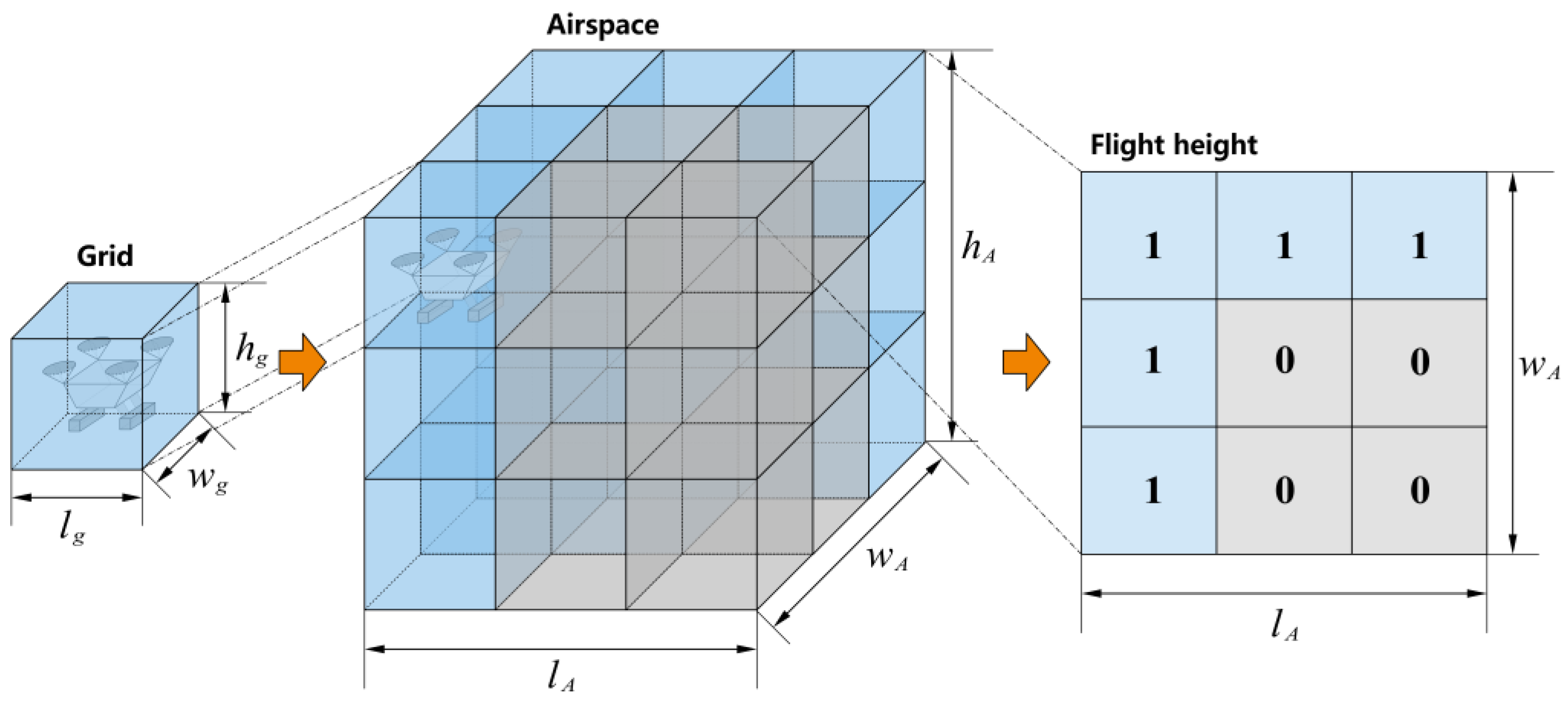
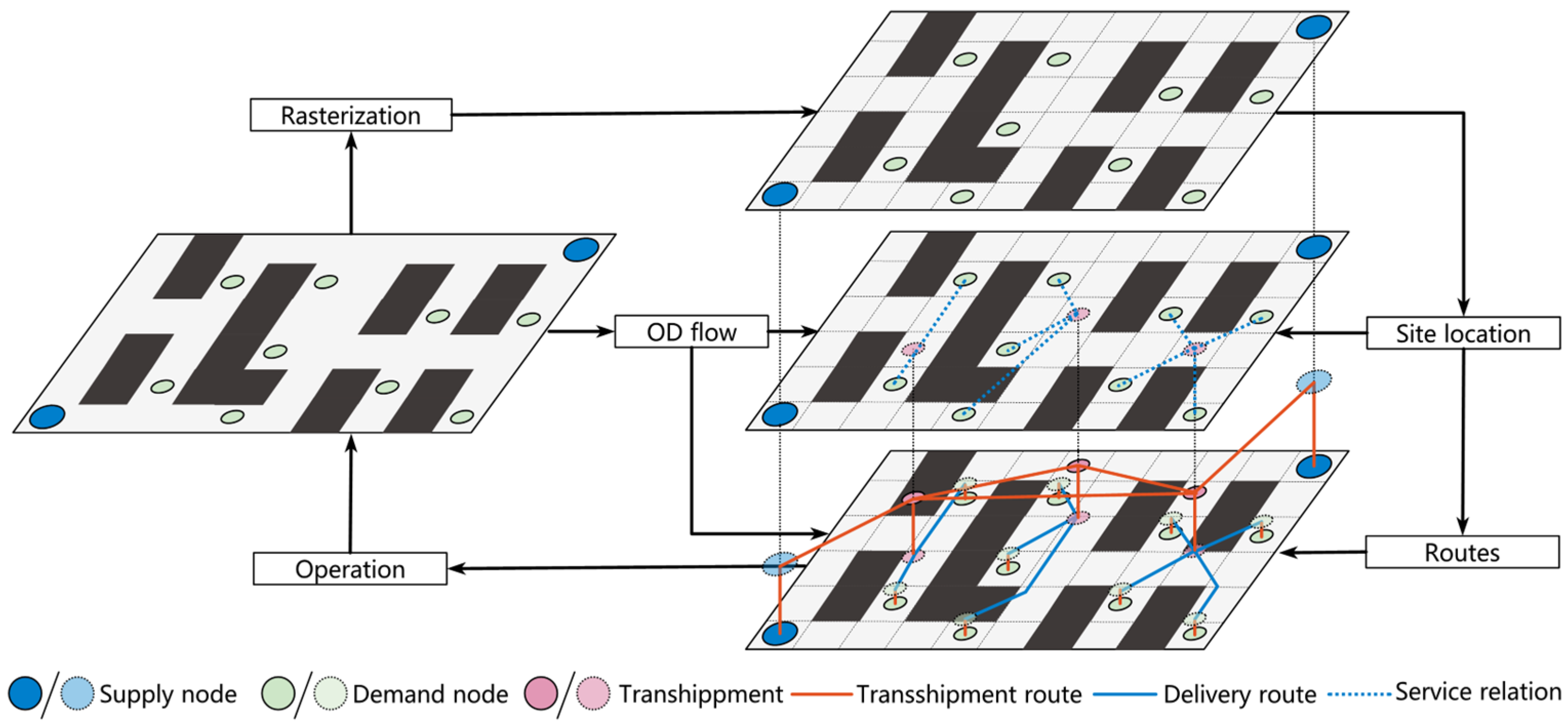
3.1.2. Rasterization of Airspace

The three-dimensional discrete modeling of the study area is carried out by using the raster method. Based on the UAV flight altitude and the obstacles in the airspace, the study area is divided into a grid pattern. Assuming the area is a cuboid with the dimensions $l_A,w_A,h_A$ and the fundamental grid dimensions are $l_g,w_g,h_g$, the airspace can be discretized into ${\displaystyle \frac{l_A}{l_g}}\times {\displaystyle \frac{w_A}{w_g}}\times {\displaystyle \frac{h_A}{h_g}}$ grids, as shown in Figure 3. Considering the UAV flight level as $h_u$, the overflight safety margin as $h_s$, and the building height as $h_o$, the characteristics of each grid are represented by the binary variable $grid\left(x,y,z\right)$.

$$grid\left(x,y,z\right)=\left\{\begin{array}{l}1,h_u-h_s>h_o\\ 0,h_u-h_s\le h_o\end{array}\right.$$

(1)

When $grid\left(x,y,z\right)=1$, it means that the UAV can fly in this grid; $grid\left(x,y,z\right)=0$ means that there is an obstacle in this grid and the UAV cannot fly.

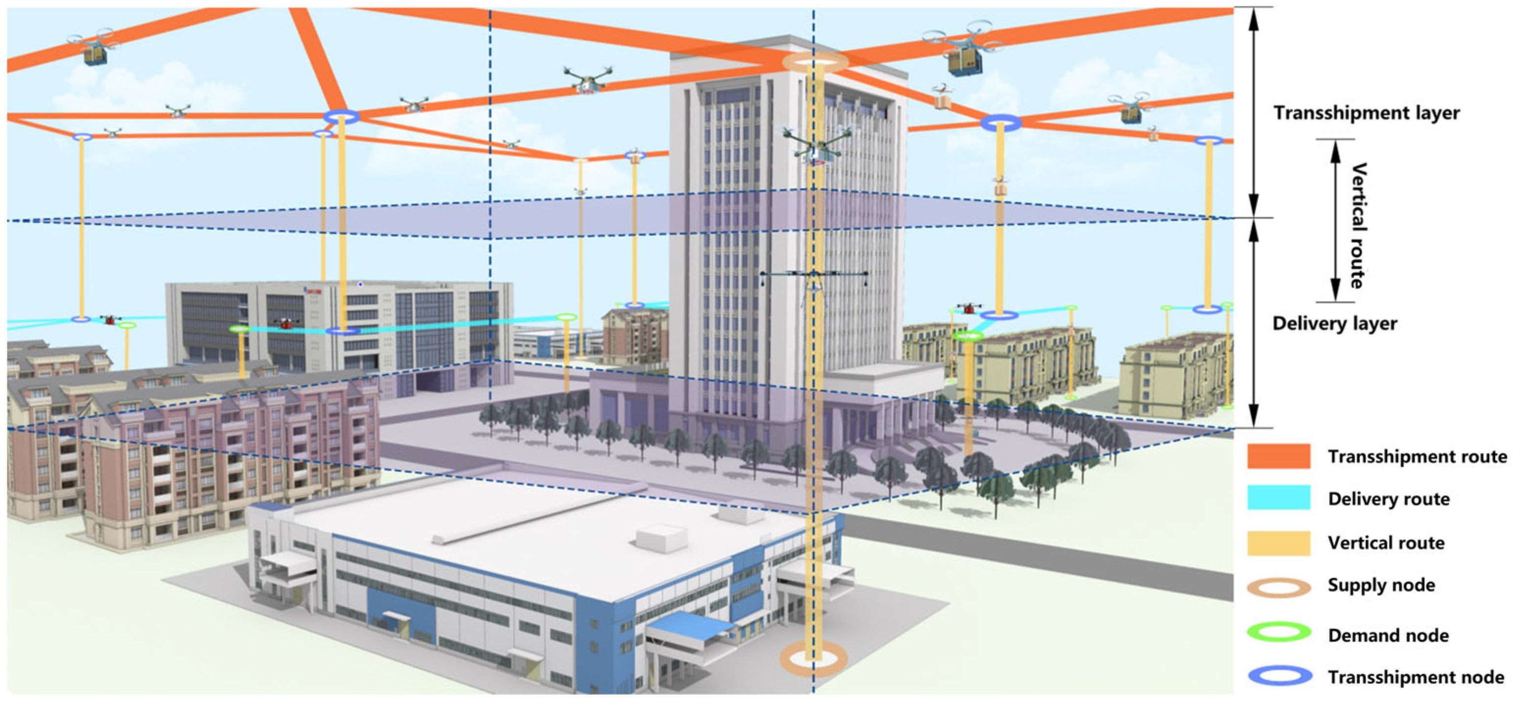
3.1.3. Route Structure

An air route is a direct flight corridor for UAVs, connecting two nodes in the network. As depicted in Figure 4, this route exhibits a bi-directional topological structure, allowing UAVs to operate in both directions while maintaining a safety separation from one another. The starting and ending points of the route are generally supply nodes, transshipment nodes, or demand nodes. According to the connectivity between nodes in the network and the needs of distribution tasks, the route can be divided into a direct route and a transit route. The direct route provides a straight connection between two nodes, and the transit route is used when the direct connection is not available. For instance, the route A-C between node A and node C serves as a direct route if the UAV performs the delivery task from node A to node C. Conversely, if a drone is assigned a task from node A to node D and there is no direct route between these nodes, the drone must utilize the route A-C as a transit route to reach its destination. In this scenario, route A-C functions as a transit route for this task.

Taking into account the aerial environment and logistics distribution tasks, along with the assumptions previously outlined, this paper proposes a hierarchical planning model to design a distribution network, as depicted in Figure 5. The network is bifurcated into a transshipment network and a delivery network, differentiated by the varying flight route altitudes and connection targets of the UAVs. The transshipment network is constructed by linking supply nodes with transshipment nodes, creating an interconnected network. The delivery network is formed by interlinking transshipment nodes with demand nodes.

The transshipment network and delivery network are set up at different altitude levels and connected by vertical routes. As the altitude increases, the airspace encounters a reduction in both the quantity and concentration of obstacles, leading to fewer turning points that require circumnavigation. Conversely, in the lower-altitude airspace, there is a higher concentration of obstacles, complicating the avoidance process and necessitating more frequent turns. The transshipment network, which experiences high drone traffic and significant operational pressure, is strategically positioned at a higher altitude. This positioning allows drones to fly more efficiently and directly from the supply nodes to transshipment nodes. Additionally, the reduced number of potential route intersections can alleviate regulatory burdens.

A more specialized delivery network is situated in the lower-altitude layer of the network. The linkage between transshipment nodes and demand nodes in the delivery network is more streamlined, with UAVs flying directly to the demand nodes without the need for intermediate transit routes. Even if route obstacle avoidance needs to be considered at the low altitude level, there are very few route intersections, reducing the collision risk and improving the delivery efficiency.

3.2. Transshipment Node Service Location Model

The main task of the service location model is to find a group of transshipment nodes which can serve all demand nodes and have better transportation efficiency in the airspace grid and to determine the appropriate service connection relationship between demand nodes and transshipment nodes.

3.2.1. Basic Definitions and Constraints

(1)

Basic definitions

Any grid without obstacles in the airspace can be considered as a feasible transshipment node. Let the set of transshipment nodes be $A$; any transshipment node is $a\left(a\in A\right)$. Let the set of demand nodes be $B$; any demand node is $b\left(b\in B\right)$, and the number of demand nodes is $n_b$.

(2)

Constraint conditions

$p_{ab}$ is a binary variable that denotes the direct service relationship between any transshipment node, $a$, and demand node, $b$, shown as follows.

$$p_{ab}=\left\{\begin{array}{l}1a\mathrm{serves}b\\ 0a\mathrm{does}\mathrm{not}\mathrm{serve}b\end{array}\right.$$

(2)

Each demand node, $b$, needs to be directly served by a transshipment node; then,

$${\displaystyle \sum _{a\in A}{p}_{ab}}=1$$

(3)

When a transshipment node is designated to serve a demand node, the pressure exerted at it becomes a critical factor. The transshipment node service pressure is calculated based on the cumulative demand of all demand nodes that the transshipment node is responsible for servicing. Let $c_b$ represent the demand size at the demand node $b$ and the maximum allowable service pressure for the transshipment node be $k_{\max }$. Consequently, the service pressure at the transshipment node is assessed to ensure it remains within the acceptable threshold, displayed as follows.

$${\displaystyle \sum _{b\in B}{p}_{ab}{c}_b}<k_{\max }$$

(4)

If $\left(x_a,y_a,z_a\right)$ are the coordinates of transshipment node $a$ and $\left(x_b,y_b,z_b\right)$ are the coordinates of demand node $b$, then the straight-line distance $\Delta d_{ab}$ between the two nodes can be calculated as

$$\Delta d_{ab}=\sqrt{{\left(x_a-x_b\right)}^2+{\left(y_a-y_b\right)}^2+{\left(z_a-z_b\right)}^2}$$

(5)

In order to avoid the demand node that the transshipment node serves being too far away, a service radius constraint is set for the transshipment node. Let the service radius of the transshipment node be $r_a$, and this constraint is expressed as

$$p_{ab}\Delta d_{ab}\le r_a$$

(6)

3.2.2. Optimization Objectives and Modeling

The optimal location of the transshipment node needs to be determined according to the location of the demand node. At the same time, it is crucial to find the service matching relationship between the transshipment node and the demand node with higher efficiency and more balanced pressure.

(1)

Minimum total service distance $Z_1$

From the perspective of distribution efficiency, the smaller the distance between the transshipment node and the demand node, the higher the efficiency of cargo transportation in the delivery network. Therefore, we hoped to shorten the distance between all transshipment nodes and their service demand nodes as much as possible. The first objective function of the model is to minimize the total service distance, expressed as

$$\min \left(Z_1\right)=\min \left({\displaystyle \sum _{a\in A}{\displaystyle \sum _{b\in B}{p}_{ab}\Delta d_{ab}}}\right)$$

(7)

(2)

Minimum transshipment node number $Z_2$

For any feasible transshipment node, according to its connection with the demand node, function $u_a$ indicates whether the node is enabled, expressed as

$$u_a=\left\{\begin{array}{ll}1& {\displaystyle \sum _{b\in B}{p}_{ab}}\ge 1\\ 0& {\displaystyle \sum _{b\in B}{p}_{ab}}=0\end{array}\right.$$

(8)

Then, the total number of enabled transshipment nodes, $n_a$, can be shown as

$$n_a={\displaystyle \sum _{a\in A}{u}_a}$$

(9)

The higher the number of transshipment nodes, the more redundant nodes and intersections there will be in the network. For airspace regulators, reducing the number of transshipment nodes can improve the regulatory efficiency and reduce operational costs, so the second objective function is to minimize the number of transshipment nodes, namely

$$\min Z_2=\min \left(n_a\right)$$

(10)

(3)

Minimum average service pressure $Z_3$

Each transshipment node is tasked with servicing a specific number of demand nodes. Ideally, the service pressure at these transshipment nodes should be minimized to enhance the operational efficiency. Consequently, the third objective function $Z_3$ can be obtained from Equation (4) to minimize the transshipment nodes’ average service pressure, expressed as

$$\min Z_3=\min \left({\displaystyle \frac{1}{n_a}}{\displaystyle \sum _{a\in A}{\displaystyle \sum _{b\in B}{p}_{ab}{c}_b}}\right)$$

(11)

By integrating the constraints and objectives, the transshipment node service location model can be obtained as follows:

$$\begin{array}{l}\min \left(Z_1,Z_2,Z_3\right)\\ s.t.\left\{\begin{array}{l}{\displaystyle \sum _{a\in A}{p}_{ab}}=1\\ {\displaystyle \sum _{b\in B}{p}_{ab}{c}_b}<k_{\max }\\ p_{ab}\Delta d_{ab}\le r_a\end{array}\right.\end{array}$$

(12)

3.3. Air Route Network Planning Model

The optimal location for the transshipment node in the airspace is determined using the above model, and then all nodes are connected through the air routes to achieve network connectivity. When selecting these air routes, it is crucial to consider not only the distance and efficiency of individual routes but also the interactions between them, as well as the overall congestion and operational status of the entire air route network. In the air route network planning model, the goal is to identify a set of air routes that ensure interconnectivity between nodes, with the distance from the supply nodes to the demand nodes falling within the flight range of UAVs. In addition, the combination of these air routes should enhance operational efficiency and safety.

3.3.1. Basic Definitions and Constraints

(1)

Basic definitions

Let the set of supply nodes be $S$; any supply node is $s\left(s\in S\right)$, and the number of supply nodes is $n_s$. Let the set of enabled transshipment nodes be $A_u\left(A_u\subset A\right)$ and any transshipment node be $a\left(a\in A_u\right)$.

When planning the route in the transshipment layer, the main consideration is the connection between the supply node and the transshipment node. For the convenience of subsequent calculation, let the waypoint set of the transshipment layer be $R_t$, which includes all supply nodes and transshipment nodes, namely

$$R_t=A_u\cup S$$

(13)

Then, the total number of waypoints $n$ can be expressed as

$$n=n_a+n_s$$

(14)

The starting and ending nodes of routes in the transshipment network can be any one of the following: a supply node and transshipment node, supply node and supply node, or transshipment node and transshipment node. $L$ represents the set of routes directly connecting any two nodes, $i,j\left(i,j\in R_t\right)$, and any route is $l_{ij}\left(l_{ij}\in L\right)$.

(2)

Constraint conditions

The binary variable $e_{ij}$ indicates whether the direct route $l_{ij}$ between node $i$ and node $j$ is enabled, which can be shown as

$$e_{ij}=\left\{\begin{array}{ll}1& l_{ij}\mathrm{is}\mathrm{used}\\ 0& l_{ij}\mathrm{is}\mathrm{not}\mathrm{used}\end{array}\right.$$

(15)

The total number of enabled routes $n_l$ is expressed as

$$n_l=\begin{array}{cc}{\displaystyle \frac{1}{2}}{\displaystyle \sum _{i\in R_t}{\displaystyle \sum _{j\in R_t}{e}_{ij}}}& i\ne j\end{array}$$

(16)

Therefore, the adjacency matrix $E_{n\times n}$ between waypoints in the transshipment layer can be constructed by $e_{ij}$, which is indicated as

$$E_{n\times n}=\left(e_{ij}\right)$$

(17)

As seen in the network topology analyzed in Section 3.1.3, not all supply nodes are directly connected to the transshipment nodes but need to go through a certain number of transit routes to reach them. If the number of transits between two nodes is too high, the delivery efficiency will be affected. Therefore, let the upper limit of the number of transits be $\tau$ and $Q_{n\times n}^{\tau }$ be the connectivity matrix under the constraint of $\tau$. $q_{ij}^{\tau }$ is an element of $Q_{n\times n}^{\tau }$, representing the number of paths connecting node $i$ and node $j$ under no more than $\tau$ transits. $Q_{n\times n}^{\tau }$ is represented as

$$Q_{n\times n}^{\tau }=\left(q_{ij}^{\tau }\right)$$

(18)

Using the adjacency matrix $E_{n\times n}$ and the identity matrix $I$, $Q_{n\times n}^{\tau }$ can be found as

$$Q_{n\times n}^{\tau }=I+{\displaystyle \sum _{\alpha =1}^{\tau +1}{\left(E_{n\times n}\right)}^{\alpha }}$$

(19)

To ensure that there are no isolated nodes in the transshipment layer, the element $q_{ij}^{\tau }$ of $Q_{n\times n}^{\tau }$ needs to satisfy the following conditions.

$$q_{ij}^{\tau }\ge 1$$

(20)

The length $d_{ij}$ of the enabled route $l_{ij}$ cannot exceed the maximum range $d_u$ of the UAV, which is expressed as

$$d_{ij}{e}_{ij}\le d_u$$

(21)

The journey of the UAV from the supply node $s$ to the demand node $b$ can be divided into three parts: in the first part, the UAV flies from the supply node $s$ to the transshipment node $a$; in the second part, the UAV flies from the transshipment node $a$ to the demand node $b$; and the third part is the take-off and landing process of the UAV for delivery.

Part I: Let $L_{sa}\left(L_{sa}\subset L\right)$ be the set of routes that the UAV passes through successively along the shortest path from supply node $s$ to transshipment node $a$ and the set size be $n_{sa}$. Let $l_{saij}^{\left(k\right)}$ be the element in $L_{sa}$, indicating that the $k$ route passed by the drone is $l_{ij}$, and $d_{saij}^{\left(k\right)}$ be the length of the route $l_{saij}^{\left(k\right)}$. The time taken to travel along the shortest path $L_{sa}$ needs to be less than the upper limit of the transit time, which can be expressed as

$$n_{sa}-1\le \tau$$

(22)

The total flight distance of the first part cannot exceed the UAV’s maximum range, namely

$${\displaystyle \sum _{k=1}^{n_{sa}}{d}_{saij}^{\left(k\right)}{e}_{ij}}\le d_u$$

(23)

Part II: In the delivery layer, the length $d_{ab}$ of the route $l_{ab}$ connecting the transshipment node $a$ and the demand node $b$ cannot exceed the UAV’s maximum range, shown as

$$\begin{array}{cc}{d}_{ab}{p}_{ab}\le d_u& a\in A_u,b\in B\end{array}$$

(24)

Assuming that the height of the transshipment route is $h$, and considering the third part, the total distance the UAV travels from the supply node $s$ to the demand node $b$ needs to be within the UAV’s maximum range. Therefore,

$${\displaystyle \sum _{k=1}^{n_{sa}}{d}_{saij}^{\left(k\right)}{e}_{ij}}+d_{ab}{p}_{ab}+2h+\Delta d_u\le d_u$$

(25)

where $\Delta d_u$ is the margin introduced to ensure flight safety.

3.3.2. Optimization Objectives and Modeling

(1)

Minimum route betweenness standard deviation $Z_4$

The route betweenness refers to the proportion of the number of times passing through a certain route in all the shortest paths to the total number of shortest paths. This paper primarily focuses on calculating the betweenness of routes in the transshipment network. For any route, $l_{ij}$, we use $l_{saij}$ to denote whether route $l_{ij}$ occurs in the shortest path $L_{sa}$, namely

$$l_{saij}=\left\{\begin{array}{cc}1& l_{ij}\in L_{sa}\\ 0& l_{ij}\notin L_{sa}\end{array}\right.$$

(26)

Let $g_{ij}$ represent the betweenness of route $l_{ij}$; then,

$$g_{ij}={\displaystyle \frac{1}{n_s{n}_a}}{\displaystyle \sum _{s\in S}{\displaystyle \sum _{a\in A}{l}_{saij}}}$$

(27)

When UAVs are tasked with delivery missions, they will naturally gravitate towards the shortest routes available. A high betweenness value of flight routes suggests that these routes are pivotal within the network, potentially drawing a significant concentration of UAVs. This can lead to a reduction in the capacity of the route as it becomes saturated with traffic. Conversely, routes with lower betweenness signify that they play a less prominent role in the network operation and may be less frequently utilized by UAVs. This could result in these routes being underutilized and idle for extended periods.

The route BSD is employed as a metric to gauge the disparity in the betweenness of these routes. By minimizing the BSD for a route, it is possible to ensure that the selected routes contribute closely to the network functionality and improve the route traffic capacity. Therefore, the minimum route BSD $Z_4$ was introduced as an objective function, which is calculated as follows.

$$\overline{g}={\displaystyle \frac{{\displaystyle \sum _{i\in R_t}{\displaystyle \sum _{j\in R_t}{g}_{ij}}}}{{\displaystyle \sum _{i\in R_t}{\displaystyle \sum _{j\in R_t}{e}_{ij}}}}}i\ne j$$

(28)

$${\delta }_g=\sqrt{{\displaystyle \frac{1}{2n_l}}{\displaystyle \sum _{i\in R_t}{\displaystyle \sum _{j\in R_t}{e}_{ij}{\left(g_{ij}-\overline{g}\right)}^2}}}i\ne j$$

(29)

$$\min Z_4=\min \left({\delta }_g\right)$$

(30)

where $\overline{g}$ is the mean value of the route betweenness and ${\delta }_g$ denotes the standard deviation of the route betweenness.

(2)

Minimum total network distance $Z_5$

In the case of covering all the nodes, a smaller total distance of the route network means that the control pressure and operation cost of the route will be relatively low, so the minimum total network distance $Z_5$ was introduced as one of the objective functions, namely

$$\begin{array}{c}\min Z_5=\min \left({\displaystyle \frac{1}{2}}{\displaystyle \sum _{i\in R_t}{\displaystyle \sum _{j\in R_t}{d}_{ij}{e}_{ij}}}+{\displaystyle \sum _{a\in A_u}{\displaystyle \sum _{b\in B}{d}_{ab}{p}_{ab}}}\right)i\ne j\end{array}$$

(31)

(3)

Minimum average non-linear coefficient $Z_6$

To improve the delivery efficiency, the distance between the supply node and demand node should be shortened as much as possible. The relationship between the actual distance and the straight-line distance is measured by the non-linear coefficient; the larger the non-linear coefficient is, the larger the actual distance is than the straight-line distance, and the delivery efficiency is relatively lower. Therefore, the minimum average non-linear coefficient $Z_6$ is regarded as one of the objective functions, which can be indicated as

$$\min Z_6=\min \left({\displaystyle \frac{1}{n_s{n}_b}}{\displaystyle \sum _{s\in S}{\displaystyle \sum _{b\in B}\frac{{\displaystyle \sum _{k=1}^{n_{sa}}{d}_{saij}^{\left(k\right)}{e}_{ij}}+d_{ab}{p}_{ab}}{\sqrt{{\left(x_s-x_b\right)}^2+{\left(y_s-y_b\right)}^2+{\left(z_s-z_b\right)}^2}}}}\right)$$

(32)

where $\left(x_s,y_s,z_s\right)$ are the coordinates of supply node $s$.

By integrating the constraints and objectives, the air route network planning model can be obtained as follows:

$$\begin{array}{l}\min \left(Z_4,Z_5,Z_6\right)\\ s.t.\left\{\begin{array}{l}{q}_{ij}^{\tau }\ge 1\hfill \\ n_{sa}-1\le \tau \hfill \\ d_{ij}{e}_{ij}\le d_u\hfill \\ d_{ab}{p}_{ab}\le d_u\hfill \\ {\displaystyle \sum _{k=1}^{n_{sa}}{d}_{saij}^{\left(k\right)}{e}_{ij}}+d_{ab}{p}_{ab}+2h+\Delta d_u\le d_u\hfill \\ i,j\in R_t\\ s\in S,a\in A_u,b\in B\end{array}\right.\end{array}$$

(33)

3.4. Indicators for Assessing the Operation of the Route Network

The operational assessment is conducted at two principal levels: those of the UAV operator and the route’s regulatory authority. From the vantage point of UAV operators, the focus is on evaluating the average flight duration for transportation tasks and the aggregate number of UAV missions required to meet delivery demands. From the perspective of route regulators, the emphasis is on scrutinizing the degree of route congestion and the magnitude of risk associated with intersections. Accordingly, this paper presents three kinds of key performance evaluation indicators.

(1)

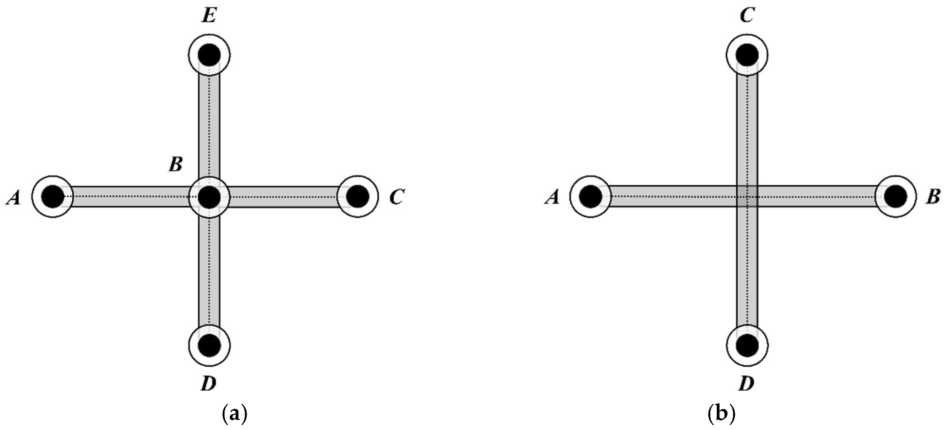
Route intersection situation

A route intersection is defined as a zone where two or more routes converge. As shown in Figure 6, intersections can be categorized into two types: functional intersections and structural intersections. The former are the transit nodes proposed in this study, where UAVs execute various heading changes at these nodes. The latter are structural sections, where UAVs pass without changing course. Within the network, an elevated count of structural intersections can lead to a considerable decrease in the UAV flight safety and an increase in regulatory challenges. As a result, this paper adopts the count of structural intersections as one of the critical indicators for assessing the safety level of the network.

(2)

Route utilization situation

It is known that the demand from demand node $b$ to supply node $s$ is $c_{sb}$ and the upper load limit and average load of a UAV are $w_{\max }$ and $w_u$, respectively. Then, on the route from the supply node $s$ to the demand node $b$ through the transshipment node $a$, the number of UAV sorties $N_{sab}$ is expressed as

$$\begin{array}{cc}{N}_{sab}=ceil\left(c_{sb}/w_u\right)& w_u\le w_{\max }\end{array}$$

(34)

where $ceil\left(\right)$ denotes rounding up.

The total number of UAV sorties $N_{sa}$ operated on the route from the supply node $s$ to the transshipment node $a$ can be further calculated as

$$N_{sa}={\displaystyle \sum _{b\in B}{N}_{sab}{p}_{ab}}$$

(35)

For any transshipment layer route, $l_{ij}$, the total passing volume $N_{ij}$ of UAVs on this route can be calculated using $N_{sa}$.

$$\begin{array}{cc}{N}_{ij}={\displaystyle \sum _{s\in S}{\displaystyle \sum _{a\in A_u}{N}_{sa}{l}_{saij}}}& i,j\in R_t\end{array}$$

(36)

The total number of UAV sorties in the transshipment layer can be shown as

$$\begin{array}{cc}{N}_{total}={\displaystyle \frac{1}{2}}{\displaystyle \sum _{i\in R_t}{\displaystyle \sum _{j\in R_t}{N}_{ij}}}& i\ne j\end{array}$$

(37)

(3)

Flight duration situation

The average flight duration refers to the mean time it takes for a UAV to traverse from the supply node to the designated demand node via the shortest path. Let the UAV’s average horizontal flight speed be denoted as $v_1$ and its vertical flight speed as $v_2$. The travel time $T_{sb}$ for the UAV from supply node $s$ to demand node $b$ can be determined as

$$T_{sb}={\displaystyle \frac{1}{v_1}}\left({\displaystyle \sum _{k=1}^{n_{sa}}{d}_{saij}^{\left(k\right)}{e}_{ij}}+d_{ab}{p}_{ab}\right)+{\displaystyle \frac{2h}{v_2}}$$

(38)

Then, the average flight duration $\overline{T}$ can be obtained as follows.

$$\overline{T}={\displaystyle \frac{1}{n_s{n}_b}}{\displaystyle \sum _{s\in S}{\displaystyle \sum _{b\in B}{T}_{sb}}}$$

(39)

4. Double-Layer Optimization Algorithm Design

In this paper, a novel “location-connection” double-layer algorithm framework is developed to address the challenges of urban UAV logistics distribution network generation. As shown in Figure 7, the framework is composed of three integral components: an upper-layer algorithm to solve the model proposed in Section 3.2, a lower-layer algorithm to solve the model proposed in Section 3.3, and operational assessment to analyze the network usage characteristics, with the methodological process delineated as follows.

Step 1: Airspace rasterization. The research airspace is discretized to identify obstacles and viable airspace. Rasterization effectively condenses the search space for nodes and enhances the speed of route development.

Step 2: Transshipment node location. The upper-layer algorithm uses the MOSA based on the Pareto frontier to ascertain the preliminary positioning of transshipment nodes and their service relationships. The transshipment node coordinates are then fed into the subsequent lower-layer algorithm.

Step 3: Route network construction. The improved cellular automated algorithm (ICA) [42] is applied to establish a route repository that interconnects all nodes, thereby setting the groundwork for route selection. The lower-layer algorithm adopts the NSGA-II to pick routes that meet the stipulated constraints and exhibit superior performance, thereby assembling the route network from the route repository using the positions of transshipment and demand nodes.

Step 4: Operational assessment. Based on the demand volume of demand nodes, a simulation operation of the route network is carried out to obtain indicators such as the total number of sorties and the operating mileage of UAVs to evaluate the network performance.

Step 5: Optimization adjustment. Further refinements are made to the transshipment nodes and routes where there is a concentration of traffic and potential for congestion, aiming to optimize the network performance.

4.1. Upper-Layer Algorithm Design

Transshipment node location is essentially a search for a set of grids that meet the constraints and have better performance in discrete airspace. Since the transshipment nodes are in the same height layer, the grid space can be simplified to a two-dimensional plane consisting of ${\displaystyle \frac{l_A}{l_g}}\times {\displaystyle \frac{w_A}{w_g}}$ grids. The solution set space of the simplified problem is still very large, assuming that from a transshipment node performing door-to-door service, there are ${\left({\displaystyle \frac{l_A}{l_g}}\times {\displaystyle \frac{w_A}{w_g}}\right)}^{n_b}$ total possibilities. Population-based evolutionary algorithms, such as genetic algorithms, immunization algorithms, etc., have the problems of inefficiency and slow convergence when solving this issue.

A simulated annealing algorithm can effectively avoid the above problems. When iterating, the algorithm only deals with two individuals each time, which not only reduces the difficulty of the algorithm but also causes the local optimal solution to jump out. Therefore, this paper adopts the MOSA to deal with the problem of transshipment node location. The MOSA introduces the concept of a Pareto frontier for multi-objective problems. By constantly comparing the dominant relationship between individuals, a set of solution clusters that can effectively dominate other individuals is finally found, which is the Pareto frontier. Then, a better solution can be found from the Pareto frontier according to certain rules. The pseudo-code for the MOSA implementation is shown in Algorithm 1.

4.1.1. Coding Strategy

As shown in Figure 8, the individual $ID=\left\{in{d}_i\left(x,y\right)\right\}$ is coded as 0–1, and the length of the individual is ${\displaystyle \frac{l_A}{l_g}}\times {\displaystyle \frac{w_A}{w_g}}$. Each gene site $in{d}_i\left(x,y\right)$ in the individual indicates whether or not the $grid\left(x,y\right)$ is selected as a transshipment node.

$$in{d}_i\left(x,y\right)=\left\{\begin{array}{l}0,\mathrm{Being}\mathrm{used}\\ 1,\mathrm{Free}\end{array}\right.$$

(40)

4.1.2. Individual Update

The individual update introduces some random perturbations based on the original individual to obtain a new individual. In the MOSA, crossover and mutation in the genetic algorithm are used for individual updating. Crossover exchanges the position of random equal-length segments in the original individual. Mutation is the reverse operation of the gene site in the individual, that is, the original $in{d}_i\left(x,y\right)=1$, and makes $in{d}_i\left(x,y\right)=0$ through mutation.

4.1.3. Metropolis Criteria

The core of this step is to use the dominance rule and acceptance probability to determine whether the new individual can replace the current individual. First, according to the constraints in Equation (12), it is judged whether the newly generated individual satisfies the constraints. If it does not meet the conditions, it is regenerated until the constraints are met.

The dominance rule is the basis for the subsequent construction of the Pareto frontier. Suppose that the objective function of the new individual $I{D}_{new}$ is $Z_u^{new}=\left\{Z_1^{new},Z_2^{new},Z_3^{new}\right\}$, the objective function of the current individual $I{D}_{old}$ is $Z_u^{old}=\left\{Z_1^{old},Z_2^{old},Z_3^{old}\right\}$, and the acceptance probability of the individual is $p_{acc}$. For any two individuals, there are three relationships between them: dominant, dominated, and equal. The comparison results between the new and old individuals are as follows:

$$\left\{\begin{array}{ll}I{D}_{new}\succ I{D}_{old}& \left(Z_1^{new}<Z_1^{old}\right)\cap \left(Z_2^{new}<Z_2^{old}\right)\cap \left(Z_3^{new}<Z_3^{old}\right)\\ I{D}_{new}\prec I{D}_{old}& \left(Z_1^{new}\ge Z_1^{old}\right)\cap \left(Z_2^{new}\ge Z_2^{old}\right)\cap \left(Z_3^{new}\ge Z_3^{old}\right)\\ I{D}_{new}=I{D}_{old}& \exists \left(Z_i^{new}<Z_i^{old}\right)\cup \left(Z_i^{new}\ge Z_i^{old}\right)\end{array}\right.$$

(41)

According to the above formula, a dominance list is made. The dominance list can reflect the performance and rank of an individual in all the solutions generated throughout the simulated annealing process. The domination list contains three parts: the number of dominant individuals $N_d\left(I{D}_i\right)$, the number of dominated individuals $N_s\left(I{D}_i\right)$, and the number of individuals of an equal rank $N_e\left(I{D}_i\right)$, namely

$$\begin{array}{l}\mathrm{case}1:I{D}_{new}\succ I{D}_{old}\left\{\begin{array}{l}{N}_d\left(I{D}_{new}\right)=N_d\left(I{D}_{new}\right)+1\\ N_s\left(I{D}_{old}\right)=N_s\left(I{D}_{old}\right)+1\end{array}\right.\\ \mathrm{case}2:I{D}_{new}\prec I{D}_{old}\left\{\begin{array}{l}{N}_s\left(I{D}_{new}\right)=N_s\left(I{D}_{new}\right)+1\\ N_d\left(I{D}_{old}\right)=N_d\left(I{D}_{old}\right)+1\end{array}\right.\\ \mathrm{case}3:I{D}_{new}=I{D}_{old}\left\{\begin{array}{l}{N}_e\left(I{D}_{new}\right)=N_e\left(I{D}_{new}\right)+1\\ N_e\left(I{D}_{old}\right)=N_e\left(I{D}_{old}\right)+1\end{array}\right.\end{array}$$

(42)

Assuming that the energy difference between the old and new individuals is $\Delta E$, the rule for calculating the probability of the acceptance of an individual according to the dominance relationship can be calculated as

$$\Delta E={\displaystyle \sum _{i=1}^3\left(Z_i^{new}-Z_i^{old}\right)}$$

(43)

$$p_{acc}=\left\{\begin{array}{l}1I{D}_{new}\succ I{D}_{old}\\ \exp \left(-\Delta E/T\right)\left(I{D}_{new}\prec I{D}_{old}\right)\cup \left(I{D}_{new}=I{D}_{old}\right)\end{array}\right.$$

(44)

Subsequently, a single random number is generated within the range of [0,1]. If this is less than $p_{acc}$, the new individual is adopted as the current solution, replacing the previous one; otherwise, the existing solution remains unchanged.

4.1.4. Algorithm Iteration

Let the initial temperature be $T_0$ and the temperature decay coefficient be $\alpha$. When the algorithm’s outer loop enters the $gen$ generation, the temperature $T$ is updated to

$$\begin{array}{cc}T={\alpha }^{gen}{T}_0& T>T_L\end{array}$$

(45)

where $T_L$ is the final temperature, and the algorithm stops updating when the temperature is less than $T_L$.

Throughout the MOSA process, all generated solutions undergo comparative and selective filtering. Let the Pareto frontier be denoted as $pareto$; then, the individuals within the solution set $pareto$ need to fulfill the following criteria.

$$pareto=\left\{I{D}_i\right\}\forall I{D}_i\in pareto,N_s\left(I{D}_i\right)=0$$

(46)

Solutions located in $pareto$ signify that they are neither dominated nor dependent on each other, and they possess advantages over all other known solutions. The score for each individual is determined by their respective objective functions. The individual with the highest score in $pareto$ emerges as the final solution. The methodology for calculating the individual score is outlined as follows.

$$p{o}_i={\displaystyle \sum _{j=1}^3\frac{\max \left(Z_j^{I{D}_i}\right)-Z_j^{I{D}_i}}{\max \left(Z_j^{I{D}_i}\right)-\min \left(Z_j^{I{D}_i}\right)}}I{D}_i\in pareto$$

(47)

4.1.5. Algorithm Flow

The process of representing the MOSA through pseudo-code is shown as follows.

Algorithm 1: MOSA
Require:
1.	The location of demand node.
2.	The grid information.
Set:
1.	Set T0 as T, input TL and decay factor $\alpha$.
Ensure:
1.	Generate a primary solution as old individual (OI) follow the Equation (40).
2.	Calculate the targets of OI.
3.	Generate the domination relationship list (DRL) and solution set (ST).
4.	While T > TL
5.	for iterating in the inner loop.
6.	Generate a new individual (NI) based on OI follow the rule in Section 4.1.2.
7.	Calculate the targets of NI.
8.	If NI does not satisfy Equation (12), repeat to row 6. Otherwise, move on.
9.	Update ST and calculate the target of NI.
10.	Compare domination relationship between NI and OI by Equation (41).
11.	Update the DRL and calculate the pacc by Equation (44).
12.	If rand(1) < pacc
13.	NI replaces OI as the current solution.
14.	end if
15.	end for
16.	Update T based on Equation (45).
17.	end while
18.	Filter the pareto solution from DRL and ST based on Equation (46).
19.	Calculate the score of pareto solution based on Equation (47).
20.	The solution with the highest score will be the final solution.

4.2. Lower-Layer Algorithm Design

The algorithm employs the ICA to search the air routes that connect any two nodes at a specific altitude level. By stratifying the routes, a comprehensive route repository is developed, which includes both transshipment and delivery routes. Once the location of the transshipment node is completed, the service relationship between the transshipment node and the demand node is established. Subsequently, it becomes a matter of allocating the appropriate delivery route from the route repository based on the service relationship. Thus, the focus of route selection optimization is primarily on the selection of transshipment routes. That is, on the basis of the known terminal delivery routes, several transshipment routes are selected from the route repository to effectively connect the supply node and transshipment node to meet the distribution demand and improve the transportation efficiency.

In this paper, the NSGA-II is used to solve the route network planning model. The NSGA-II is an evolutionary algorithm for solving multi-objective optimization problems, which uses a fast non-dominated sorting method to rank individuals in a population. By introducing a crowding comparison operator to maintain the diversity of the population, the algorithm can explore the solution space more comprehensively.

4.2.1. Coding Strategy

As shown in Figure 9, a set of transshipment routes is extracted from the route repository. The chromosome $C{R}_i=\left\{c{r}_{ij}\right\}$ of each individual adopts binary coding, representing the use of a group of transshipment routes, and the chromosome length is $C_{n_s+n_a}^2$. The gene $c{r}_{ij}$ indicates whether the $j$ route on the chromosome $i$ is enabled or not. The population size of each generation is $G$.

$$c{r}_{ij}=\left\{\begin{array}{l}0,\mathrm{route}j\mathrm{is}\mathrm{free}\\ 1,\mathrm{route}j\mathrm{is}\mathrm{used}\end{array}\right.$$

(48)

Whether each individual satisfies the constraints in Equation (33) is determined, and if it does, its objective function value $Z_j^{C{R}_i}$ is computed. If it does not, each of the three objective function values of the chromosome is assigned an extremely large number, $M$, to ensure that the individual will not be selected for the next generation.

4.2.2. Genetic Operations

There are two main steps in genetic manipulation: roulette selection and crossover and mutation. Roulette selection indicates that each individual is copied into the offspring with a certain probability. Crossover and mutation are similar to the MOSA and will not be repeated here.

(1)

Roulette selection

After obtaining the objective function values, the cumulative selection probability of an individual is calculated. Firstly, the objective function values of the individuals are normalized separately to ensure that their dimensions are consistent, and then the score $p{o^{\prime }}_i$ of each individual is calculated as

$$p{o^{\prime }}_i=\left\{\begin{array}{l}{\displaystyle \sum _{j=4}^6\frac{\max \left(Z_j^{C{R}_i}\right)-Z_j^{C{R}_i}}{\max \left(Z_j^{C{R}_i}\right)-\min \left(Z_j^{C{R}_i}\right)}}{Z}_j^{C{R}_i}\ne M\\ 1/M{Z}_j^{C{R}_i}=M\end{array}\right.$$

(49)

Then, the cumulative selection probability $p{a}_i$ of the individual can be calculated as

$$p{a}_i=\left\{\begin{array}{l}\begin{array}{cc}p{o^{\prime }}_i/{\displaystyle \sum _{i=1}^{G}p{o^{\prime }}_i}& i=1\end{array}\\ \begin{array}{cc}p{a}_{i-1}+p{o^{\prime }}_i/{\displaystyle \sum _{i=1}^{G}p{o^{\prime }}_i}& i>1\end{array}\end{array}\right.$$

(50)

During the execution of roulette selection, a random number, $rand\left(1\right)$, in the range [0,1] is generated, and the position of this random number in the roulette cumulative probability is determined. If $p{a}_{i-1}<rand\left(1\right)\le p{a}_i$, the individual $C{R}_i$ is chosen for reproduction. Conversely, if either $rand\left(1\right)\le p{a}_1$ or $rand\left(1\right)>p{a}_G$, the individuals located at the start and end boundaries of the population are selected. By performing $G$ roulette operations, a filial population of the same size as the parental population is generated.

(2)

Crossover and mutation

Crossover is an operation in which parts of the chromosomes of two individuals are exchanged so that the individuals form a new trait. Mutation is the inversion of a gene on a chromosome. This part is similar to the principle in Section 4.1.2 and will not be repeated here.

4.2.3. Metropolis Criteria

Similarly to the rules mentioned in Section 4.1.3, there is also non-dominated sorting in the NSGA-II. This mechanism broadens the selection range when producing the next generation of individuals by mixing parental and filial individuals to form a new group. The detailed steps are as follows.

Step 1: Assess whether each individual of the parental and filial generations satisfies the constraints given in Equation (33) after crossover and mutation. If yes, calculate the objective function values. If not, assign an exceedingly high value, $M$, to the objective function values to indicate that the individual is not dominated.

Step 2: Determine the dominance relationship between any two chromosomes, $C{R}_i$ and $C{R}_j$, by applying the following criteria.

$$\left\{\begin{array}{ll}C{R}_i\succ C{R}_j& \left(Z_4^{C{R}_i}<Z_4^{C{R}_j}\right)\cap \left(Z_5^{C{R}_i}<Z_5^{C{R}_j}\right)\cap \left(Z_6^{C{R}_i}<Z_6^{C{R}_j}\right)\\ C{R}_i\prec C{R}_j& \left(Z_4^{C{R}_i}\ge Z_4^{C{R}_j}\right)\cap \left(Z_5^{C{R}_i}\ge Z_5^{C{R}_j}\right)\cap \left(Z_6^{C{R}_i}\ge Z_6^{C{R}_j}\right)\\ C{R}_i=C{R}_j& \exists \left(Z_n^{C{R}_i}<Z_n^{C{R}_j}\right)\cup \left(Z_n^{C{R}_i}<Z_n^{C{R}_j}\right)\end{array}\right.$$

(51)

Similarly to in Section 4.1.3, the dominance of each individual in the population can be obtained according to the number of individuals dominated by the chromosome $N_d\left(C{R}_i\right)$, the number of dominated individuals $N_s\left(C{R}_i\right)$, and the number of individuals of the same rank $N_e\left(C{R}_i\right)$.

Step 3: Classify the individuals according to the number of dominated individuals $N_s\left(C{R}_i\right)$. The smaller the $N_s\left(C{R}_i\right)$ of an individual, the more dominant it is in the group, and these individuals have a higher rank. Individuals with $N_s\left(C{R}_i\right)=0$ are the optimal individuals in the population and are ranked first. With an increase in $N_s\left(C{R}_i\right)$, the individual disadvantage gradually increases and the rank decreases.

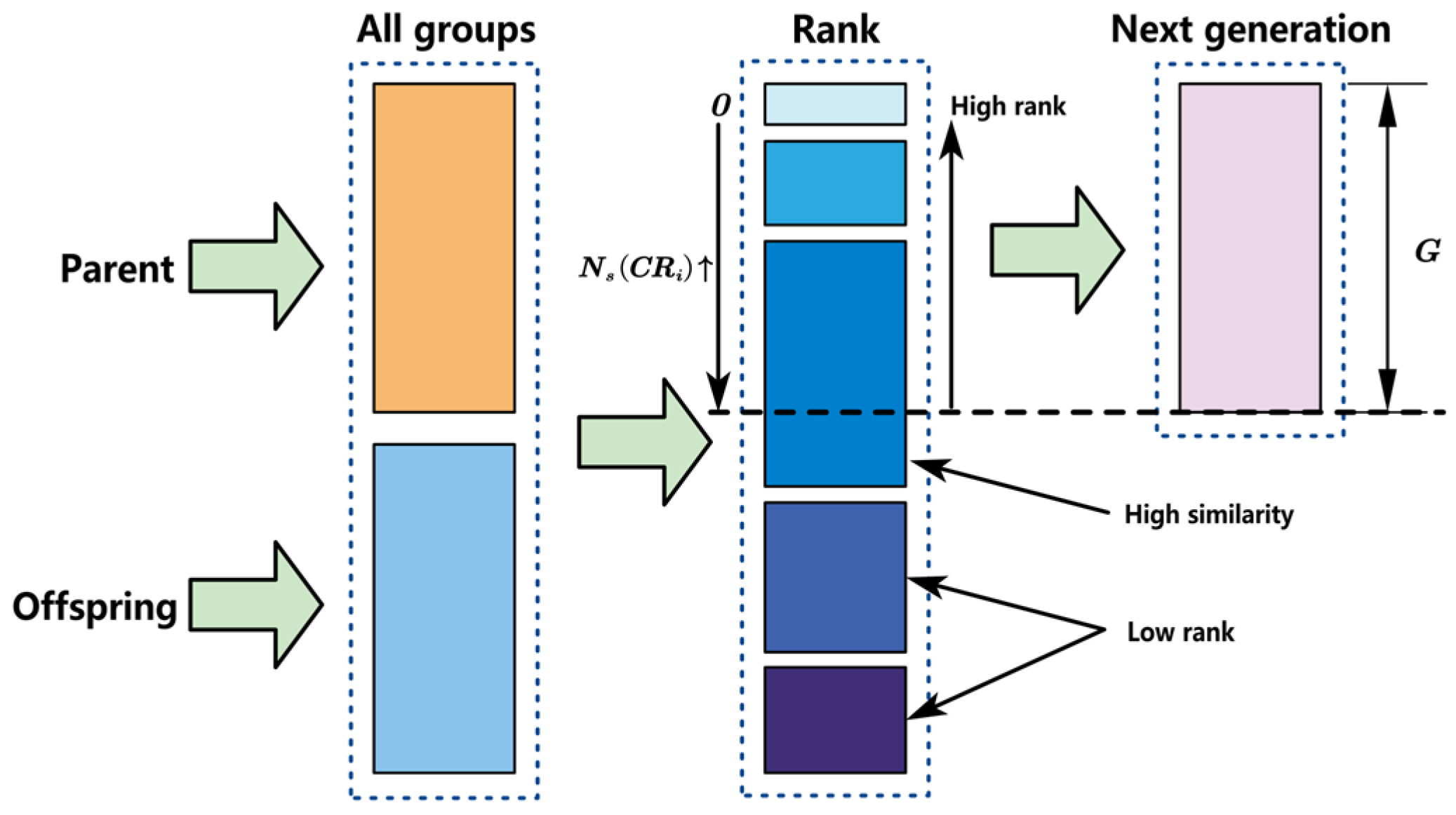
4.2.4. Population Renewal

When selecting individuals to enter the next generation, firstly, individuals with $N_s\left(C{R}_i\right)=0$ will be directly copied into the next generation; secondly, the remaining individuals will be selected according to the individual rank from large to small. When the cumulative number of individuals in the pre-selected class exceeds the size of the original population, the individuals in that class are selected using similarity ranking.

Similarity is used to measure the degree of similarity between individuals and can reflect the position of an individual in the solution space. When an individual has high similarity in the population, it reflects the tendency of the population to be homogeneous. If individuals with higher similarity are generally selected for the next generation, there is a possibility of coming across the local optimal solution and early convergence. To increase the diversity of the population and further fully search for other locations in the solution space, it is necessary to select individuals with less similarity to enter the next generation.

Suppose there exist $S$ individuals that need to be compared in terms of similarity. First, the similarity between any two of these individuals needs to be calculated as follows.

$$sim\left(C{R}_m,C{R}_n\right)={\displaystyle \sum _{j=1}^{C_{n_s+n_a}^2}c{r}_{mj}\odot c{r}_{nj}}$$

(52)

where $\odot$ is the Boolean operator and $sim\left(C{R}_m,C{R}_n\right)$ indicates the number of genes that individual $C{R}_m$ shares with individual $C{R}_n$.

Then, the similarity of individual $C{R}_m$ in the population to be compared is calculated as follows.

$$sim\left(C{R}_m\right)={\displaystyle \frac{{\displaystyle \sum _{n=1}^{S-1}sim\left(C{R}_m,C{R}_n\right)}}{{\displaystyle \sum _{m=1}^S{\displaystyle \sum _{n=1}^{S-1}sim\left(C{R}_m,C{R}_n\right)}}}}$$

(53)

The method to obtain the next generation is shown in Figure 10.

5. Simulation Experiment

5.1. Scene Setting

An area in Nanjing was selected as the test scenario for simulation analysis. The area was about 1800 m wide and 2025 m long. There were 58 nodes in the region, including 2 supply nodes and 56 demand nodes. The building data and elevation data of this area were extracted according to Google Earth, and after rasterizing the airspace, $390\times 450$ grids were obtained at the same flight level, and each grid size was $4.5 \mathrm{m}\times 4.5 \mathrm{m}$. Combined with consideration of the local population distribution and logistics needs, through field investigation, we presumed that the total demand of the 56 demand nodes was around 8880 kg, of which the demand for supply node 1 was 4940 kg, and the demand for supply node 2 was 3940 kg. The demand of each node is shown in

Table 1. Variation in logistics distribution demand between nodes.

Demand Node	Distribution Demand (kg)		Demand Node	Distribution Demand (kg)
	Supply Node 1	Supply Node 2		Supply Node 1	Supply Node 2
1	60	80	29	120	120
2	80	80	30	120	80
3	40	60	31	120	100
4	100	60	32	80	60
5	100	60	33	120	80
6	120	100	34	180	140
7	100	100	35	80	40
8	120	80	36	100	60
9	60	60	37	80	40
10	80	80	38	80	80
11	60	40	39	60	80
12	40	40	40	60	80
13	80	60	41	80	80
14	40	40	42	60	40
15	60	40	43	100	80
16	60	40	44	40	60
17	80	60	45	80	40
18	100	120	46	60	40
19	60	40	47	40	60
20	120	80	48	140	80
21	80	40	49	100	60
22	100	60	50	60	60
23	100	80	51	80	40
24	120	120	52	80	80
25	120	120	53	100	40
26	100	80	54	100	80
27	120	120	55	120	40
28	100	100	56	100	60

.

The simulation experiments were carried out using MATLAB 2022a, and the environment was an 11th Gen Intel(R) Core(TM) i7-11800H@2.30GHz CPU 2.30GHz. The main parameters were set as shown in

Table 2. Simulation parameters.

Variable	Value
$k_{\max },w_{\max }$	1000 kg, 20 kg
$\tau$	5 times
$r_a,d_u,\Delta d_u,h$	200 m, 3000 m, 200 m, 90 m
$v_1,v_2$	10 m/s, 3 m/s

.

5.2. Experimental Results

The route network planning environment is shown in Figure 11a. Based on the building environment, the low-altitude airspace was rasterized, and the distribution demand was estimated according to the population distribution. By solving the double-layer planning model, 17 transshipment nodes were obtained in the upper model, and a route repository with 171 transshipment routes and 56 delivery routes was generated in the lower model, as shown in Figure 11b.

The final route network is shown in Figure 12, which consisted of 26 transshipment routes and 56 delivery routes. In the following section, the location of transshipment nodes and the results of network planning are analyzed in detail. The red numbers in the figure indicate the code of the transshipment node and the black numbers indicate the code of the demand node.

5.3. Numerical Analysis

(1)

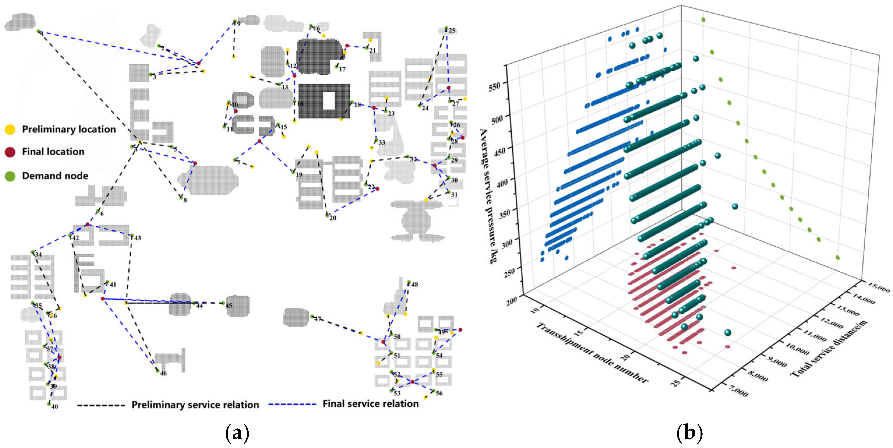
Transshipment node location analysis

In the upper model, the initial temperature $T_0$ was set to 100, and the temperature decay coefficient $\alpha$ was 0.995. After 1380 iterations, a Pareto frontier with 732 solutions was finally obtained. The final solution with the highest score was selected from the Pareto front, which enabled there to be 17 transshipment nodes with a total service distance of 7088.9 m and an average service pressure of 522.35 kg. Each transshipment node served an average of 3.3 demand nodes, and the service relationship is shown in

Table 3. Transshipment node service relationship.

Transshipment Node	Service Demand Node	Delivery Cargo Volume (kg)
		From Supply Node 1	From Supply Node 2
A1	B35, B36, B37, B38, B39, B40	460	380
A2	B6, B34, B42, B43	460	360
A3	B41, B44, B45, 46	260	220
A4	B4, B5, B8	320	200
A5	B1, B2, B3, B9	240	280
A6	B10, B11	140	120
A7	B7, B15, B19	220	180
A8	B12, B13, B14, B16	220	180
A9	B17, B21	160	100
A10	B18, B23, B33	320	280
A11	B20, B22	220	140
A12	B47, B48, B50, B51	320	240
A13	B52, B53, B55, B56	400	220
A14	B29, B30, B31, B32	440	360
A15	B24, B25, B27	360	360
A16	B49, B54	200	140
A17	B26, B28	200	180

.

The location results for the transshipment nodes are shown in Figure 13a. The yellow dots are the initial transshipment nodes, and the black dotted lines are the initial service relationship. The red dots are the transshipment node locations of the final solution, and the blue dotted lines are the service relationships of the final solution. By comparing the initial solution with the final solution, it was found that the locations and service connections of the final solution were more reasonable. In the initial location selection, a large number of transshipment nodes were used, with a total scale of 37. The total service distance was as high as 15,450 m, while the distance between some transshipment nodes and demand nodes was large, and the terminal distribution efficiency is low. Although the average service pressure of the transshipment nodes was relatively small, the distance between some transshipment nodes was small, which indicated that there was a possibility of combining multiple transshipment nodes with low service pressure and close spacing. In the final solution, the number of global transshipment nodes was reduced to 17, and the total service distance was reduced to 7088.9 m. Although the service pressure was increased, the distribution efficiency was effectively improved on the whole. Regarding the distribution of transshipment nodes, when the number of demand nodes in an area was relatively concentrated, the number of transshipment nodes was greater, and the service pressure on the transshipment nodes in this area was significantly greater than that on other transshipment nodes.

Figure 13b shows the Pareto frontier of the upper model. The different colored points on the coordinate plane are planar projections of the Pareto frontier, showing the relationship between the different objective functions, where the number of transshipment nodes is negatively correlated with the total service distance and average service pressure, while the total service distance and average service pressure are positively correlated. When the number of demand nodes served by the transshipment nodes is large, considering the limit case, that is, the one-to-one correspondence of a transshipment node with a service demand node, the total service distance tends toward zero. As the number of transshipment nodes decreases, the transshipment nodes cannot take care of every demand node they serve, which will inevitably increase the service distance between the transshipment nodes and some demand nodes, thus increasing the total service distance. At the same time, when the transshipment node only serves one demand node, the service pressure on each transshipment node will not be too great. However, with a reduction in the number of transshipment nodes, the number of demand nodes served by the same transshipment node will increase, which will lead to a significant increase in the overall service pressure.

Therefore, the number of transshipment nodes is the core factor controlling the upper model. By adjusting the number of transshipment nodes, the total service distance and the average service pressure can be effectively controlled.

(2)

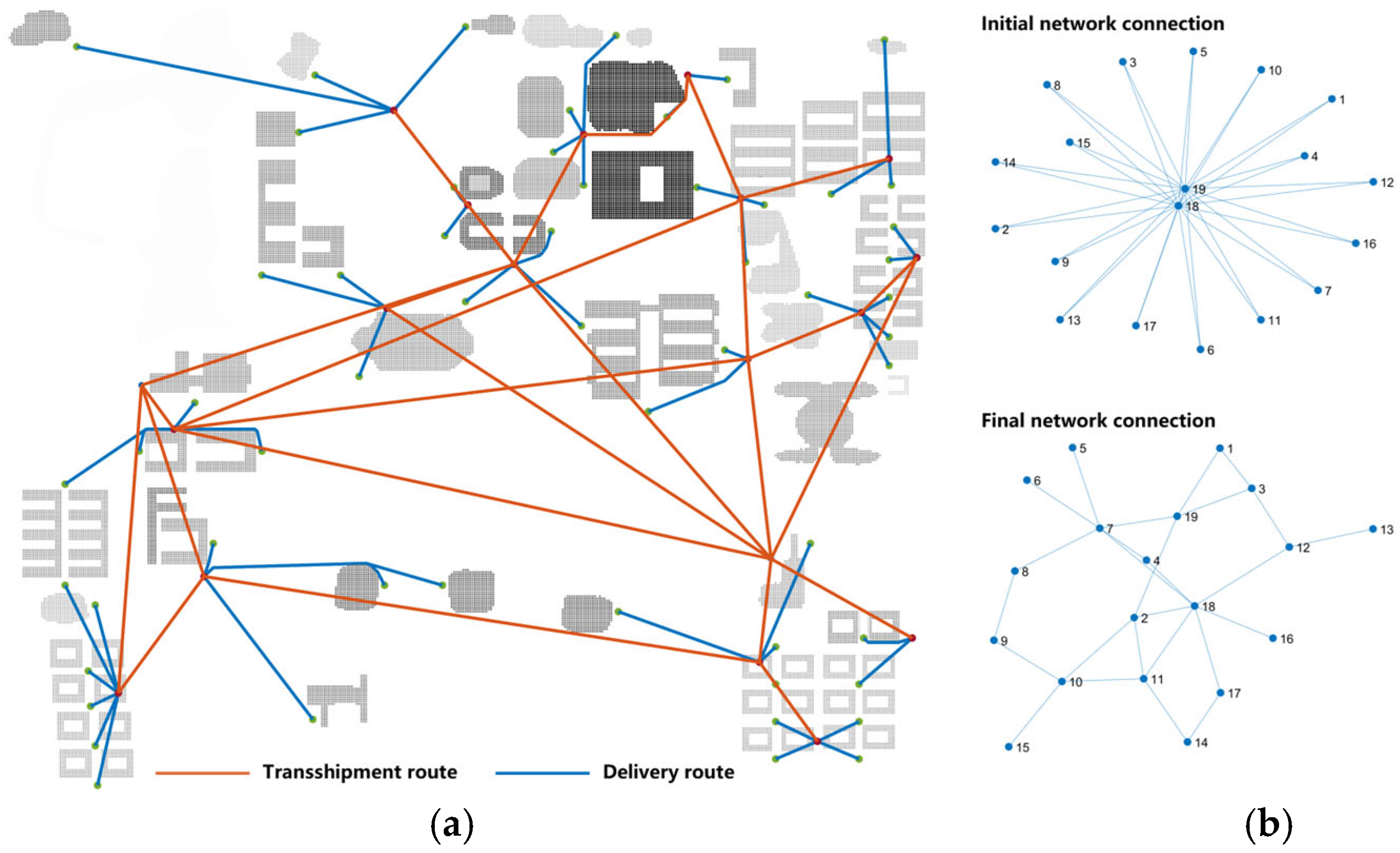
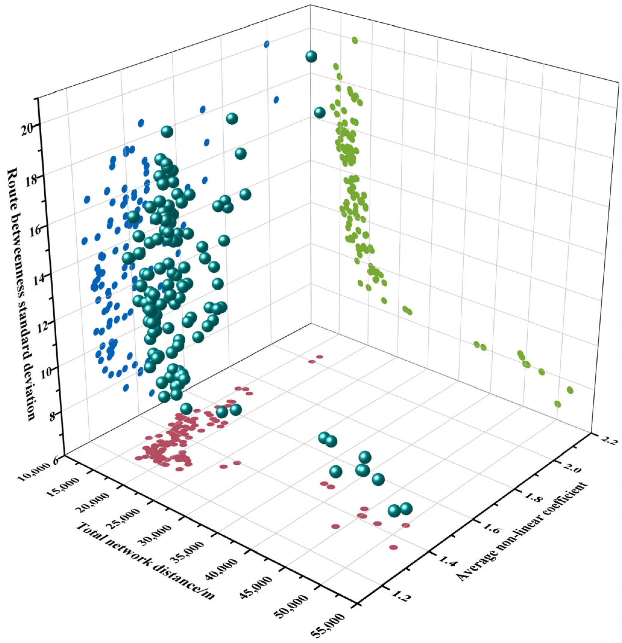
Route network structure analysis

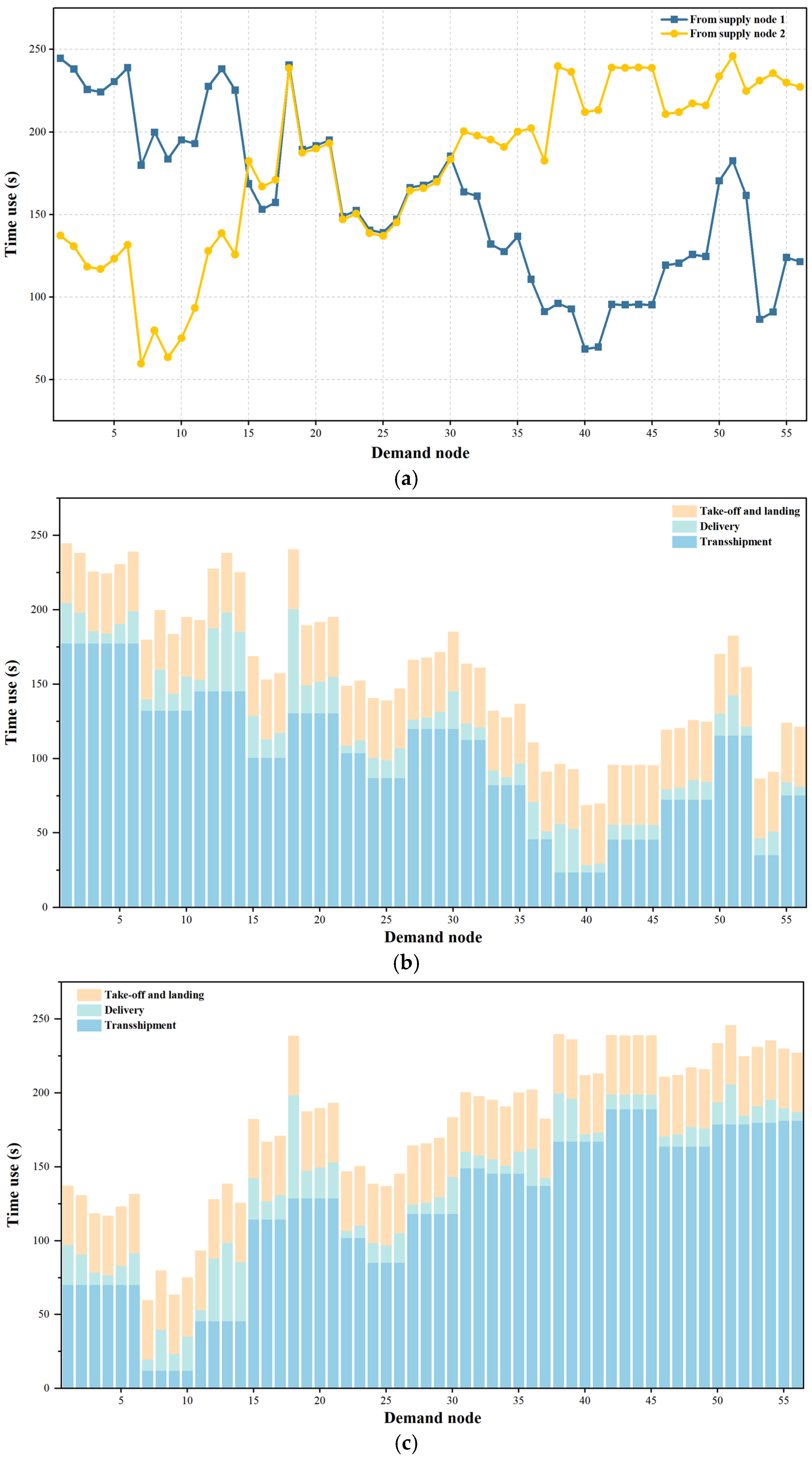
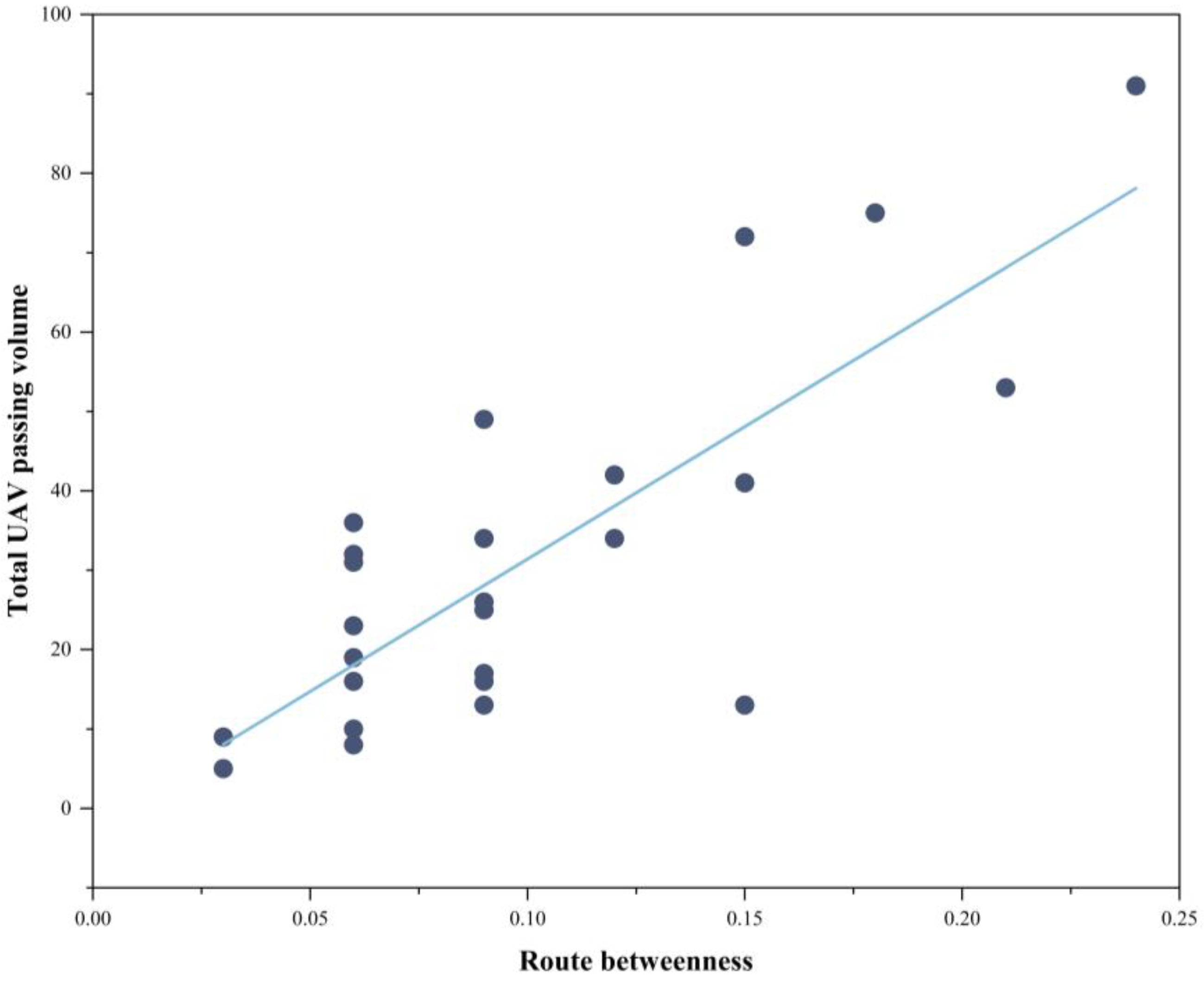
In the lower model, the population size of the NSGA-II was 100, and the probabilities of crossover and mutation were 1% and 0.1%, respectively. Through 500 population evolutions, the optimal solution for each generation was extracted, and these optimal solutions were sorted in a non-dominated manner to obtain a Pareto frontier containing 135 solutions, as shown in Figure 14. The final solution with the highest score was extracted from the Pareto front, and the transshipment route service relationship is shown in

Table 4. Transshipment layer route assignment information.

Supply	Transshipment	Route	Distance (m)	Supply	Transshipment	Route	Distance (m)
S1	A1	S1, A12, A3, A1	1775.25	S2	A1	S2, A1	701.78
S1	A2	S1, A2	1323.3	S2	A2	S2, A2	122.07
S1	A3	S1, A12, A3	1452.07	S2	A3	S2, A3	455.47
S1	A4	S1, A4	1006.88	S2	A4	S2, A7, A4	1143.29
S1	A5	S1, A7, A5	1306.02	S2	A5	S2, A7, A5	1286.68
S1	A6	S1, A7, A6	1038.02	S2	A6	S2, A7, A6	1018.68
S1	A7	S1, A7	870.01	S2	A7	S2, A7	850.68
S1	A8	S1, A7, A8	1200.96	S2	A8	S2, A7, A8	1181.62
S1	A9	S1, A11, A10, A9	1125.74	S2	A9	S2, A7, A8, A9	1491.52
S1	A10	AS1, A11, A10	823.05	S2	A10	S2, A2, A10	1455.85
S1	A11	S1, A11	457.74	S2	A11	S2, A2, A11	1372.35
S1	A12	S1, A12	236.33	S2	A12	S2, A3, A12	1671.21
S1	A13	S1, A12, A13	455.47	S2	A13	S2, A3, A12, A13	1890.35
S1	A14	S1, A11, A14	724.29	S2	A14	S2, A2, A11, A14	1638.9
S1	A15	S1, A11, A10, A15	1155.46	S2	A15	S2, A2, A10, A15	1788.26
S1	A16	S1, A16	354.15	S2	A16	S2, A2, A18, A16	1799.52
S1	A17	S1, A17	753.96	S2	A17	S2, A2, A11, A14, A17	1812.17

. The final route network had a total distance of 25,525 m, a non-linear coefficient of 1.47, and a route BSD of 17.74. As shown in Figure 14a, in the transshipment network, 26 routes enabled the connection of 2 supply nodes and 17 transshipment nodes, with a total distance of 14,452 m. In the delivery network, 17 transshipment nodes and 56 demand nodes were connected by 56 routes, with a total distance of 9332 m. In addition, there were 75 vertical routes with a total distance of 1740 m connecting the two layers of the network.

Figure 14b shows the topological relationship between nodes in the transshipment layer. In the initial transshipment network, the supply node and the transshipment node were set to be directly connected, the non-linear coefficient was close to 1, and the transshipment route BSD was 0. However, the total distance of the transshipment network was 35,823 m, and there were many structural intersections, which made the operation of the transshipment route very risky. With the number of enabled transshipment routes gradually decreasing, the network scale also decreased, and the total distance of the final transshipment route dropped to 14,452 m, which was 59.6% lower than that of the initial solution. The number of structural intersections was reduced from 102 in the initial solution to 4, with a decrease rate of 96%. At this time, some transshipment nodes needed to be reached through transit routes, which increased the route’s non-linear coefficient and the route BSD, indicating that it is necessary to sacrifice a certain amount of distribution efficiency to reduce the network scale and improve the overall safety performance.

Figure 15 shows the Pareto front of the lower model. The total network distance is negatively correlated with the route BSD and the non-linear coefficient, while the non-linear coefficient is positively correlated with the route BSD. When the total network distance is higher, a greater number of routes are enabled, and the non-linear coefficient is close to 1. When the total network distance decreases, the non-linear coefficient increases sharply, because there is no direct route between some transshipment nodes and supply nodes, and they need to be reached through a certain transit route. Similarly, if there is a direct route between the supply node and the transshipment node, then each route is the shortest route between the two nodes, and the route BSD tends toward 0. As the number of routes decreases, the usage of each route in the network is different, resulting in an increase in the route BSD, which reflects the restrictive relationship between the network efficiency and scale.

Therefore, the total network distance is the core parameter of the lower model, and choosing the right route is the key to reducing the network scale, improving the transportation efficiency, and reducing route crossing. By controlling the non-linear coefficient, the decrease in transportation efficiency caused by excessively reducing the total network distance can be effectively avoided. By controlling the route BSD, this can balance the importance of each route in the overall network, so that the use of routes is more balanced.

(3)

Operational evaluation of network

In terms of the route network’s traffic efficiency, the average flight durations from supply node 1 and supply node 2 to the 56 demand nodes were 157.51 s and 177.91 s, the longest flight durations were 244.59 s and 245.84 s, and the shortest flight durations were 68.58 s and 59.7 s, respectively. The flight durations for each demand node are shown in Figure 16. The dark blue column, light blue column, and orange column, respectively, represent the flight duration of the first, second, and third parts. According to the three parts of the flight duration for each demand node, the UAV distribution time was mainly spent on the transshipment route, and the delivery route and the take-off and landing route were not long. Therefore, the key to improving the efficiency of UAV distribution is to ensure a smooth transshipment route.

In terms of logistics transportation, in order to meet the distribution needs of 56 demand nodes with a total of 8840 kg of goods, a total of 442 UAV sorties were deployed. The average single-mission time was 165.01 s, the overall mission flight distance was 483,170 m, and the average flight distance of a single mission was 1088 m. Furthermore, the transshipment route betweenness and the UAVs’ total passing volume were analyzed, and the relationship between them is shown in Figure 17. It can be seen from the figure that there was a strong positive correlation between route betweenness and the UAV passing volume. The total UAV passing volume on transshipment routes was 845, the average passing volume of each route was 10.3, and the standard deviation of the passing volume among routes was 22.3. Since the UAV gives priority to the route with the shortest total distance when selecting the distribution path, in the early stage of route planning, by controlling the route BSD, the use of each route is relatively average, thus reducing the potential congestion as much as possible. In addition, the UAV passing volume is also related to the transshipment node connected to it. If the service pressure of the transshipment node is high, the UAV passing volume on the route will also increase.

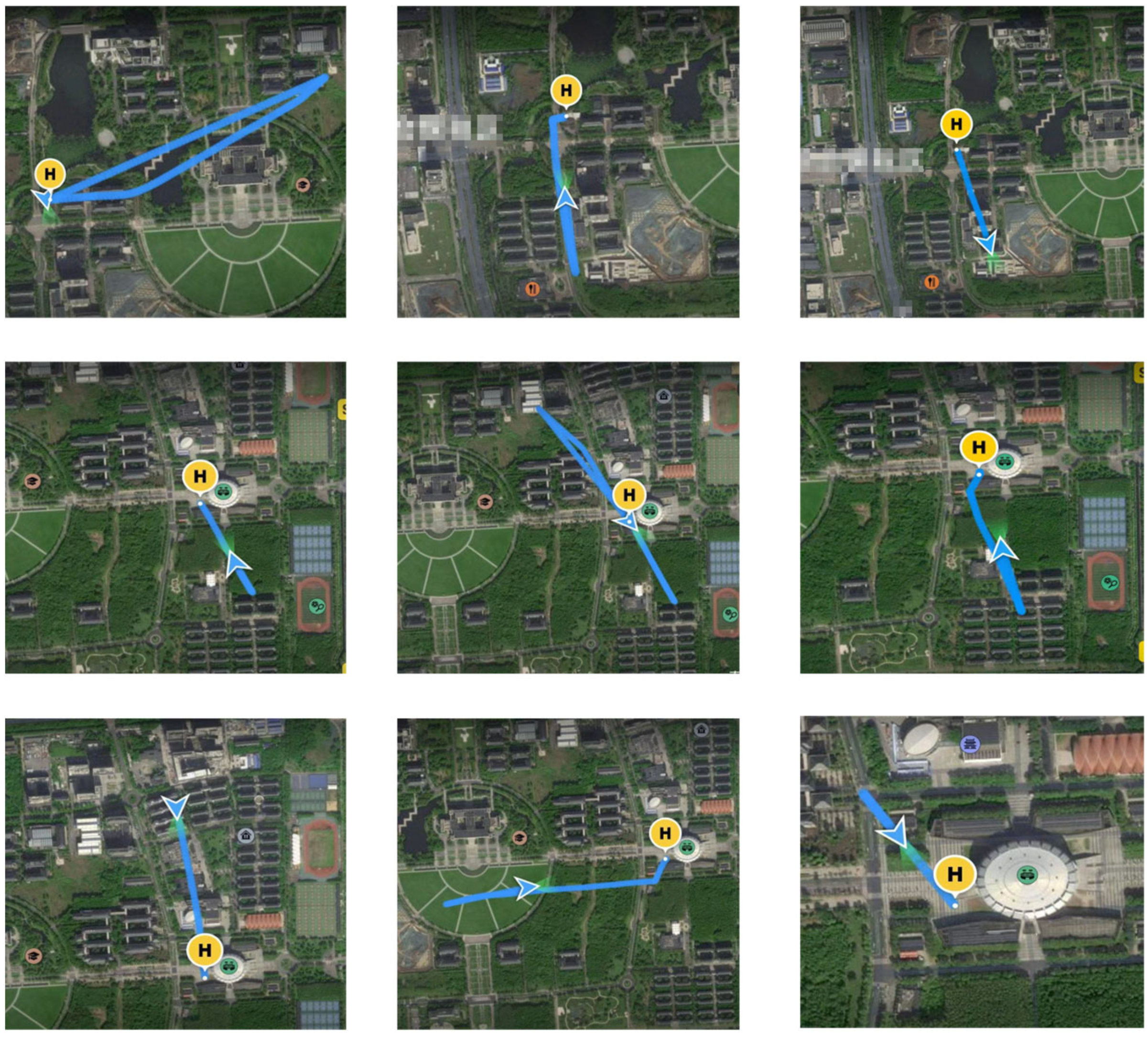
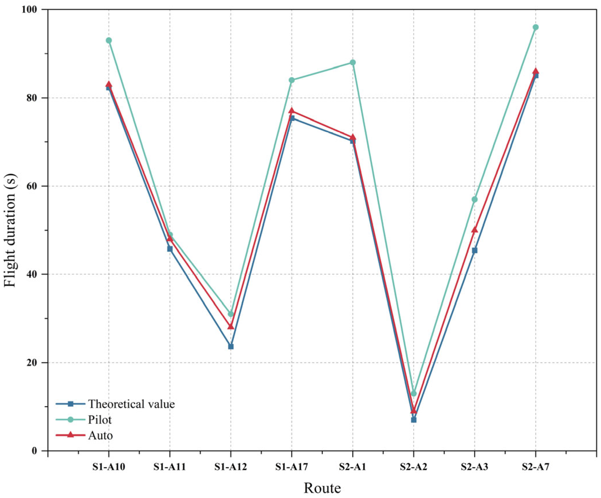
5.4. Route Flight Test

To further validate the rationality of the route planning, we selected eight routes in the transshipment layer from two supply nodes, respectively. We then conducted experimental flights using UAVs based on the DJI platform. The flight environment was characterized by sunny days and a wind force of level 2 from the southwest. The specific flight scenarios are depicted in Figure 18. The drones and obstacles are shown in the red boxed lines in the figure. Additionally, some of the routes intercepted at the DJI platform are illustrated in Figure 19. The H symbol in the figure indicates the set-up take-off and landing points.

Four flights were conducted on each route, comprising two flights operated by a human pilot and two flights executed by the autonomous route planner. The average flight time for each test route was calculated to yield specific comparative results, which are presented in Figure 20.

The flight results indicate that the theoretical values were lower than both the human pilot’s flight time and the UAV’s autonomous flight time. The difference between the human pilot’s flight time and the theoretical value was more pronounced, while the autonomous flight time closely approximated the theoretical value, with an average deviation of merely 2.15 s. All test routes could effectively avoid obstacles to ensure the safe flight of the drone. Considering the flight’s environmental conditions and communication delays, we can conclude that the simulation parameters fundamentally correspond to real-world demands.

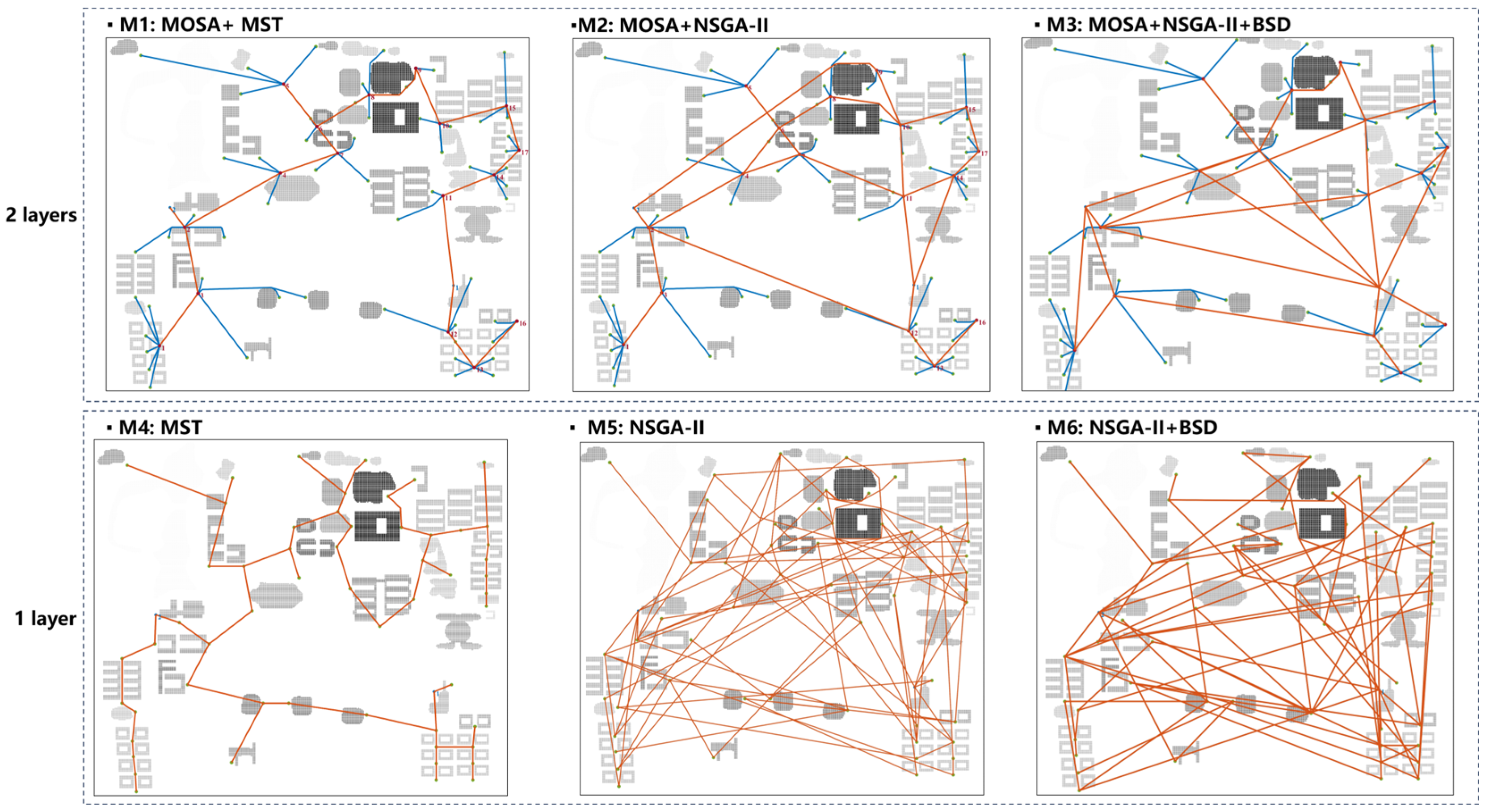
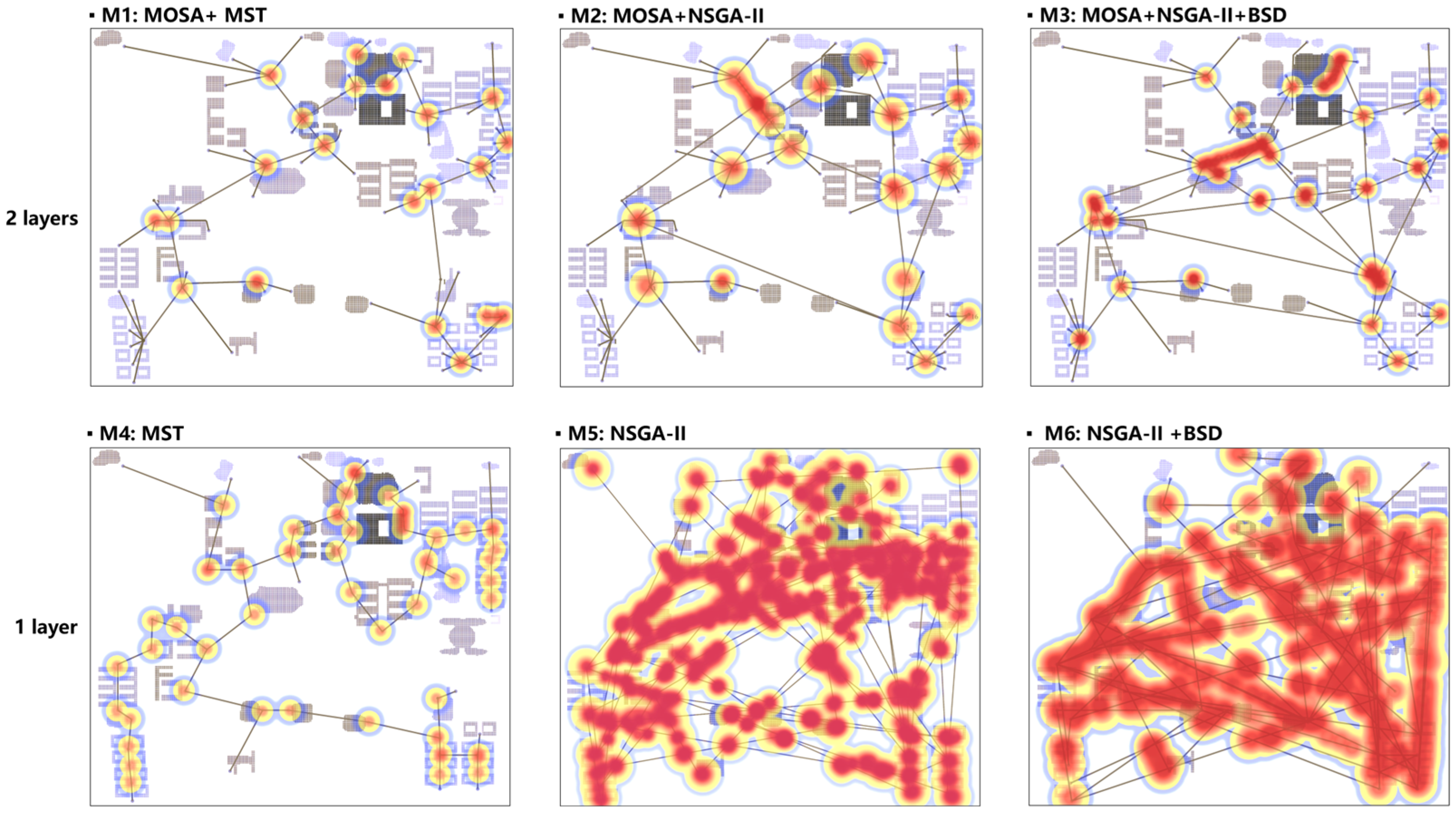
5.5. Comparison Tests

In this section, we describe how six comparative experiments were set up, and the main variables were controlled as follows.

(1)

Route network structure.

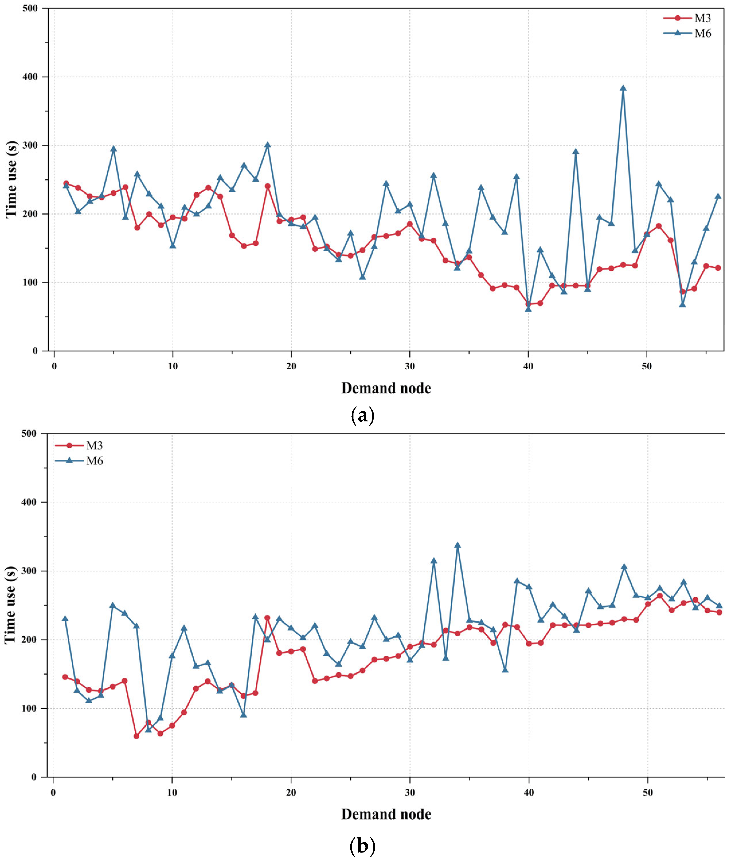
In the context of the same simulation experiment, this paper describes how we compared the single-layer route structure presented in the literature [40] with the double-layer route structure proposed herein. The aim was to elucidate the superiority and safety of the double-layer route structure by examining and contrasting the network parameters.

(2)

Route selection method and flight performance.

The MST algorithm [43] was compared with the NSGA-II utilized herein. The objective was to investigate which algorithm offers a superior strategy for route selection, both in single-layer and double-layer route networks. Furthermore, by comparing the operational efficiencies, the aim was to verify that the two-layer network structure boasts a more efficient distribution capability than the single-layer structure.

(3)

Route betweenness standard deviation effectiveness.

The role of the route BSD in mitigating potential congestion risks was explored by comparing its use as an objective function in both double-layer and single-layer route networks.

(4)

Sensitivity analysis.

The impact of the BSD factor on various networks was examined by incrementally increasing the demand in a uniform manner as well as randomly on a local scale.

Based on the above three types of variable control, the results of the route network under different conditions were obtained as shown in Figure 21, and the variable control and operation evaluation results of the network are shown in

Table 5. Results of operation evaluation and comparison of route network.

Item		Method
		M1	M2	M3	M4	M5	M6
Variable control	Layers	2	2	2	1	1	1
	Method	MST	NSGA-II	NSGA-II	MST	NSGA-II	NSGA-II
	BSD	-	NO	YES	-	NO	YES
Network structure	Size of route dataset	227 *	227 *	227 *	1653	1653	1653
	Total distance (m)	22,026	21,527 *	25,525	23,650	67,355	68,150
	Transshipment (m)	10,384	9884.4 *	14,452	20,170	63,875	64,670
	Delivery (m)	9332	9332	9332	-	-	-
	Take-off/landing (m)	2310 *	2310 *	2310 *	3480	3480	3480
	Route BSD	0.201	0.172	0.051 *	0.365	0.075	0.054
	Non-linear coefficient	1.88	1.47	1.34 *	2.88	1.78	1.59
	Intersection number	0 *	1	4	0 *	142	128
Logistics efficiency	Average flight duration (s)	250.38	175.23	167.71 *	281.96	199.81	220.09
	From supply node 1 (s)	259.3	172.03	157.51 *	329.43	195.28	212.01
	From supply node 2 (s)	241.47	178.43	177.91 *	190.92	205.25	228.16
UAV operation	Total task flight distance (m)	839,390	519,500	483,170 *	955,220	709,560	737,700
	Total UAV passing volume	1581	1110	800 *	2034	1213	1101
	Average route passing volume	21.36	13.87	9.75 *	18.01	28.20	24.3
	Standard deviation of passing volume	55.23	42.67	22.3	92.62	25.21	19.18 *

*: optimal value in four sets of experiments.

.

5.5.1. Analysis of Route Network Structure

Comparing experiments highlighted that the route database for the single-layer structure was more intricate than that for a double-layer structure, with the database size of the double-layer route being a mere 13.7% the size of the single-layer one. In the location model for the double-layer route, once the transshipment point is established, planning the delivery layer routes can be achieved. Therefore, in the planning model, the only task is to determine the optimal combination of routes in the transshipment layer. In contrast, for single-layer routes, there is no separation between transshipment and delivery functions; each route effectively handles both tasks simultaneously. Consequently, when optimizing route combinations, single-layer routes have a longer genetic code, a larger search space, and slower algorithm convergence, and it becomes more difficult to identify superior solutions.

In terms of the route distance, the double-layer structure was substantially smaller than the single-layer structure. The comparison between M3 and M6 showed a total distance reduction of up to 62.5%, and the non-linear coefficient was also significantly improved, indicating higher operational efficiency for the double-layer structure.

Figure 22 shows the location and concentration of all intersections. Double-layer routes had significantly fewer structural intersections than single-layer routes. In the figure below, the red area marks the locations of intersections (including functional and structural intersections). M6 had as many as 128 structural intersections, while a double-layer route reduced this number to just 4. This pattern was not only observed in M3 and M6 but also consistently across other experiments, with double-layer routes consistently having far fewer structural intersections than single-layer routes. This means that double-layer routes provide a safer operating environment than single-layer routes.

5.5.2. Analysis of Route Selection Method and Flight Performance

By comparing experiment M3 and M1, it is clear that although the total distance obtained using the MST algorithm was slightly shorter than that obtained using the NSGA-II, the NSGA-II obtained a route network with a smaller non-linear coefficient and route BSD by slightly sacrificing its mileage advantage. In terms of logistics distribution, the average flight durations of the route networks obtained by M3 and M6 were 82.67 s and 61.87 s faster than those of M1 and M4, respectively. Moreover, the delivery time for nearly every demand point was shorter than that obtained using the MST algorithm. Regarding the total task flight distance, M3 and M6 achieved shorter distances to fulfill distribution demands, with reduction rates of 42.4% and 29.4% compared to M1 and M4, respectively.

By comparing different network structures, it is evident that the double layer achieves better flight performance. Figure 23a,b show the average flight duration from supply node 1 and supply node 2 to each demand node in M3 and M6. The expressway mode of the transshipment layer in M3 enhanced the distribution efficiency. Consequently, the average flight duration in M3 was significantly shorter than that in M6, with a reduction of 24% of the average flight duration.

In the single-layer structure, demand points closer to the supply point experience a shorter flight time due to a more direct link. However, the double-layer structure involves two steps—transshipment and delivery—which can relatively increase the time for demand points that are closer to the supply node. From a global perspective, the transshipment layer in the double-layer structure is more efficient, with fewer transfers and a more stable overall performance. In contrast, the single-layer structure requires multiple transit routes, which significantly diminishes the distribution efficiency. From this, we can infer that in future route planning research, it may be beneficial to consider the supply node as also fulfilling part of the transshipment point’s function. This would allow for direct distribution to closer demand points, thereby optimizing the overall distribution process.

In terms of route operation, the total task flight distance of M3 was also notably less than that of M6, effectively reducing operational costs and completing distribution tasks with fewer UAV sorties.

Nevertheless, double-layer structures are not without drawbacks. The standard deviation of the UAV passing volume is marginally higher in a double-layer structure compared to a single-layer one. This stems from the separation of distribution and transshipment functions in the double-layer structure. Once the demand is met, the delivery routes become idle. In contrast, in the single-layer structure, the airway handles both transshipment and distribution. Even after demand satisfaction, it can still serve as a transit route for other demand points, thus resulting in a lower standard deviation of the usage frequency for single-layer airways than double-layer ones. Consequently, future research could focus on optimizing the link structure of delivery layer routes to enhance their utilization efficiency.

5.5.3. Analysis of Route BSD Effectiveness

The bar charts in Figure 24 depict the number of UAV passes for each route, with the double-layer routes representing the transshipment layer. As the colors deepen and the columns get taller, it indicates an increase in usage. The red dashed box highlights the route with the highest usage. Among the models, M1, M2, M4, and M5 do not utilize the BSD as an optimization objective, while M3 and M6 incorporate the BSD as one of their objective functions.

In M1, M2, M4, and M5, there were significant disparities in the total UAV passing volume, with the maximum difference in usage reaching as high as 102 and 93 times. However, when the BSD was integrated into the algorithm, as seen in M3 and M6, there was a marked reduction in the column heights, and the maximum difference in usage decreased to 78 and 41.

By comparing experiment M3 and M2, it can be seen that the total distance of M3 was slightly higher than that of M2, and the non-linear coefficient of M3 was smaller. In terms of logistics efficiency, that of M3 was significantly better than that of M2, and the average flight duration was 7.52 s shorter. In terms of UAV operation, the average passing volume of M3 was relatively lower and more balanced as a whole. For example, in M3 and M2, the routes S2 and A2 were enabled at the same time, and both routes had the largest passing volume of UAVs. However, the passing volume of route S2-A2 in M2 was as high as 192, compared to 91 in M3, which means that the potential congestion of the M3 network was lower.

However, specifically concerning network M2 and M3, given the bias in the demand volume, it could not be conclusively proven that the improvement in the operating condition could be solely attributed to the BSD factor. Therefore, we further substantiated the role of the BSD factor through sensitivity analyses.

5.5.4. Analysis of Sensitivity Effectiveness

The impact of the BSD factor on the sensitivity of double-layer network operations was examined through three methods: a uniformly increasing demand (UI), a locally randomly increasing demand (LI), and an equilibrial increase in demand (EI). The results are presented in Figure 25, which comprehensively compares three key indicators: the standard deviation of the passing volume, the total task flight distance, and the total UAV passing volume. In all three scenarios, the demand was increased in increments of 20 kg, with a maximum increment reaching 200 kg.

In the UI scenario, as the demand increased, all metrics showed improvement, yet the extent of this improvement varied significantly. The standard deviation of the passing volume for M2 increased much more significantly than that for M3. Specifically, the standard deviation for M2 exceeded 100 when the demand increment reached 100 kg. In contrast, for M3, which incorporated the BSD factor, the standard deviation of the passing volume remained below 100 even when the demand increment reached 200 kg. Similarly, the increase in the total task flight distance and the total UAV passing volume for M3 were notably smaller than those for M2.

In the LI scenario, each time 28 demand points were randomly selected, the same random sampling points were used across different route networks. The results indicated that the trends of the indexes were relatively consistent with those observed in the UI scenario. This showed that random variation still could not eliminate the disadvantage of M2. Nevertheless, it was still necessary to further rule out network differences that may have arisen due to the deviation in the initial demand.

Therefore, to mitigate the impact of preliminary demand deviations on route usage, the initial demand at each demand point was standardized to 20 kg in the EI scenario. In this case, route usage deviation was solely associated with the number of services at the transshipment nodes. Since M2 and M3 utilized the same transshipment nodes, the deviation in the route passing volume was exclusively linked to the BSD factor. The results demonstrated that, although the initial difference between the two was minimal and growth was slower than in the UI scenario, the overall performance of M2 remained inferior to that of M3 as the demand escalated. This trend aligns with the findings from the previous two sets of experiments.

Although demand bias does lead to the intensive use of some routes, the BSD factor can balance and enhance the role of the selected routes within the overall network. This allows drones to have a greater selection of optimal paths when delivering to different demand points, thereby avoiding route congestion that results from an over-reliance on single-path choices.

In summary, comparing the four route network planning methods from M1 to M6, the double-layer network structure is better than the single-layer network, and the intelligent algorithm in this paper is more reasonable than the MST algorithm in route selection, and the route BSD can effectively promote the balance of route selection. Furthermore, from comparing actual flights with theoretical calculations, we believe the simulation parameters are reasonable.

As we introduced in the background, the transshipment route in the double-layer network can be compared with an expressway in the ground road network, which speeds up the delivery of goods, effectively reduces the number of structural intersections, and ensures the safety of route operation. The lower delivery route directly connects the transshipment node with the demand node, which reduces unnecessary transit procedures and makes the distribution process simpler. Through the combination of upper and lower routes, the double-layer network structure embodies the characteristics of a simple structure, high efficiency, and safe operation.

6. Conclusions

Facing the future transportation needs of logistics UAVs, this paper proposes an urban logistics UAV route network planning method for the last-mile delivery problem. Considering the needs of different stakeholders and the complexity of the large-scale mixed operation of UAVs, combined with the demand characteristics of residents and the operation service mode of service providers, a double-layer urban low-altitude UAV logistics route network was designed. Evaluation indexes were established in terms of safety and efficiency to analyze the performance of the route network. The main contributions of this work are as follows:

(1) Aiming to address the phenomenon of many structural intersections and slow logistics efficiency in the construction of traditional route networks, the distribution mode of the “supply node—transshipment node—demand node” was put forward, and a layered route network structure was planned. The upper transshipment network composed of supply nodes and transshipment nodes was designed as the expressway of logistics distribution, and the lower delivery network composed of transshipment nodes and demand nodes was designed as the direct distribution channel.

(2) Aiming to address the issue of the location of the transshipment node under complex airspace conditions, this paper fully considers the service scope, operating pressure, and overall scale of the transshipment node and puts forward the transshipment node service location model. The experimental results show that the model can effectively determine the optimal location of transshipment nodes in the airspace and match the optimal service relationship between them and the demand nodes.

(3) Aiming to address the problem of route planning for large-scale UAV operation, a network planning model was proposed to reduce the route scale and the potential congestion risk, and improve the logistics distribution efficiency. The experimental results show that the model can effectively connect supply nodes, transshipment nodes, and demand nodes and fully meet the distribution needs of various stakeholders within the UAV cruising range.

(4) Aiming at verifying the feasibility of route planning, we selected eight transshipment layer routes to carry out actual flight tests. The results show that the actual flight time was very close to the theoretical calculation time. Thus, the approach presented in this paper can be credible to a certain extent.

(5) Through comparative experiments, we found that compared with the traditional single-layer route network structure, the proposed route network structure can effectively reduce the total network distance and mitigate the intersection risk. Compared with the traditional algorithm, the intelligent algorithm adopted in this paper has a more reasonable route structure and more efficient logistics distribution. The route BSD index can make the route use more balanced and effectively alleviate the potential operation congestion of the route.

In summary, the route network planning framework proposed in this study is helpful to the standardized, efficient, and safe operation of a large-scale urban UAV logistics network. The UAV operation environment considered in this paper is mainly complex urban obstacles. In the future, the flight performance of UAVs under different meteorological conditions can be further explored, and the influence of special weather on the route network can be studied. In addition, in view of the limitations of the current communication coverage and UAV automation capability, this paper only carried out the actual flight tests on a single route. In subsequent research, it will be possible to expand the UAV flight environment and carry out large-scale UAV route network flight tests to analyze the network performance, and sensor-based hardware systems can be implemented for real-time flight status monitoring, enabling the comprehensive safety assessment and operational integrity verification of the network. Our analysis also revealed the inherent advantages of single-layer networks in mitigating route congestion. This advantage can be effectively integrated into the subsequent optimization of double-layer networks. In addition, we will further explore the application of the double-layer network structure in scenarios such as drone–rider delivery systems and urban high-voltage power line inspection.

References

1. Zhang, H.; Zou, Y.; Zhang, Q.; Liu, H. Future urban air mobility management: Review. Acta Aeronauti. Astronaut. Sin. 2021, 42, 82–106. [Google Scholar]
2. Chung, S.H. Applications of smart technologies in logistics and transport: A review. Transp. Res. Part E Logist. Transp. Rev. 2021, 153, 102455. [Google Scholar] [CrossRef]
3. NASA. Urban Air Mobility (UAM) Market Study. 2018. Available online: https://ntrs.nasa.gov/api/citations/20190001472/downloads/20190001472.pdf (accessed on 10 September 2024).
4. Liao, X.; Qu, W.; Xu, C.; He, H.; Wang, J.; Shi, W. A review of urban air mobility and its new infrastructure low-altitude public routes. Acta Aeronauti. Astronaut. Sin. 2023, 44, 6–34. [Google Scholar]
5. Li, C.; Qu, W.; Li, Y.; Huang, L.; Wei, P. Overview of traffic management of urban air mobility (UAM) with eVTOL aircraft. J. Traffic Transp. Eng. 2020, 20, 35–54. [Google Scholar]
6. Gharibi, M.; Boutaba, R.; Waslander, S.L. Internet of drones. IEEE Access 2016, 4, 1148–1162. [Google Scholar] [CrossRef]
7. Hu, Z.; Chen, H.; Lyons, E.; Solak, S.; Zink, M. Towards sustainable UAV operations: Balancing economic optimization with environmental and social considerations in path planning. Transp. Res. Part E Logist. Transp. Rev. 2024, 181, 103314. [Google Scholar] [CrossRef]
8. Gugan, G.; Haque, A. Path planning for autonomous drones: Challenges and future directions. Drones 2023, 7, 169. [Google Scholar] [CrossRef]
9. ICAO. Innovation Driving Sustainable Aviation. 2021. Available online: https://chinaerospace.oss-cn-beijing.aliyuncs.com/uploads/2021/11/26/x13XY_Innovation%20Driving%20Sustainable%20Aviation%20-%20November%202021.pdf (accessed on 20 October 2024).
10. Holden, J.; Goel, N. Fast-Forwarding to a Future of on Demand Urban Air Transportation; Uber Elevate: San Francisco, CA, USA, 2016. [Google Scholar]
11. Rothfeld, R.; Balac, M.; Ploetner, K.O.; Antoniou, C. Agent-based simulation of urban air mobility. In Proceedings of the Modeling and Simulation Technologies Conference, Kissimmee, FL, USA, 8–12 January 2018; AIAA: Reston, VA, USA, 2018. [Google Scholar]
12. Darshan, C.; Avinash, U.; Miguel, F. Maximum coverage capacitated facility location problem with range constrained drones. Transp. Res. Part C Emerg. Technol. 2019, 99, 1–18. [Google Scholar]
13. Vascik, P.D.; Hansman, R.J. Development of vertiport capacity envelopes and analysis of their sensitivity to topological and operational factors. In Proceedings of the AIAA SciTech 2019 Forum, San Diego, CA, USA, 7–11 January 2019; AIAA: Reston, VA, USA, 2019. [Google Scholar]
14. Fu, M.; Rothfeld, R.; Antoniou, C. Exploring preferences for transportation modes in an urban air mobility environment: Munich case study. Transp. Res. Rec. 2019, 2673, 427–442. [Google Scholar] [CrossRef]
15. Qian, X. Research on Optimization Model of Coordinated Location and Layout of Urban Logistics UAV Landing and Landing Sites. Master’s Thesis, Nanjing University of Aeronautics and Astronautics, Nanjing, China, 2021. [Google Scholar]
16. Zhang, H.; Feng, D.; Zhang, X.; Liu, H.; Zhong, G.; Zhang, L. Urban logistics unmanned aerial vehicle vertiports layout planning. J. Transp. Syst. Eng. Inf. Technol. 2022, 22, 207–214. [Google Scholar]
17. Fadhil, D.N. A GIS-Based Analysis for Selecting Ground Infrastructure Locations for Urban Air Mobility. Ph.D. Thesis, Technical University of Munich, Munich, Germany, 2018. [Google Scholar]
18. Salama, M.R.; Srinivas, S. Collaborative truck multi-drone routing and scheduling problem: Package delivery with flexible launch and recovery sites. Transp. Res. Part E Logist. Transp. Rev. 2022, 164, 102788. [Google Scholar] [CrossRef]
19. Gao, J.; Zhen, L.; Laporte, G.; He, X. Scheduling trucks and drones for cooperative deliveries. Transp. Res. Part E Logist. Transp. Rev. 2023, 178, 103267. [Google Scholar] [CrossRef]
20. Cao, Y.; Chen, H. Research on truck and drone joint distribution scheduling based on cluster. Comput. Eng. Appl. 2022, 58, 287–294. [Google Scholar]
21. Kuo, R.J.; Lu, S.H.; Lai, P.Y.; Mara, S.T.W. Vehicle routing problem with drones considering time windows. Expert Syst. Appl. 2022, 191, 116264. [Google Scholar] [CrossRef]
22. Zhou, Y.; Su, Y.; Xie, A.; Kong, L. A newly bio-inspired path planning algorithm for autonomous obstacle avoidance of UAV. Chin. J. Aeronaut. 2021, 34, 199–209. [Google Scholar] [CrossRef]
23. Niu, Y.; Yan, X.; Wang, Y.; Niu, Y. 3D real-time dynamic path planning for UAV based on improved interfered fluid dynamical system and artificial neural network. Adv. Eng. Inform. 2024, 59, 102306. [Google Scholar] [CrossRef]
24. Hu, X.; Wu, Y. Risk-based discrete multi-path planning method for UAVs in urban environments. Chin. J. Aeronaut. 2021, 42, 463–474. [Google Scholar]
25. Rojas Viloria, D.; Solano-Charris, E.L.; Muñoz-Villamizar, A.; Montoya-Torres, J.R. Unmanned aerial vehicles/drones in vehicle routing problems: A literature review. Int. Trans. Oper. Res. 2021, 28, 1626–1657. [Google Scholar] [CrossRef]
26. Zhao, Q.; Lu, F.; Wang, L.; Wang, S. Research on drones and riders joint take-out delivery routing problem. Comput. Eng. Appl. 2022, 58, 269–278. [Google Scholar]
27. Lu, F.; Jiang, R.; Bi, H.; Gao, Z. Order distribution and routing optimization for takeout delivery under drone-rider joint delivery mode. J. Theor. Appl. Electron. Commer. Res. 2024, 19, 774–796. [Google Scholar] [CrossRef]
28. Shao, Q.; Li, J.; Li, R.; Zhang, J.; Gao, X. Study of urban logistics drone path planning model incorporating service benefit and risk cost. Drones 2022, 6, 418. [Google Scholar] [CrossRef]
29. Karaman, S.; Frazzoli, E. Sampling-based algorithms for optimal motion planning. Int. J. Robot. Res. 2011, 30, 846–894. [Google Scholar] [CrossRef]
30. Lavalle, S.M.; Kuffner, J.J. Rapidly-exploring random trees: Progress and prospects. Algorithm. Comput. Robot. New Dir. 2001, 5, 293–308. [Google Scholar]
31. Li, J.; Liu, H.; Lai, K.K.; Ram, B. Vehicle and UAV collaborative delivery path optimization model. Mathematics 2022, 10, 3744. [Google Scholar] [CrossRef]
32. Shen, L.; Hou, Y.; Yang, Q.; Lv, M.; Dong, J.; Yang, Z.; Li, D. Synergistic path planning for ship-deployed multiple UAVs to monitor vessel pollution in ports. Transp. Res. Part D Transp. Environ. 2022, 110, 103415. [Google Scholar] [CrossRef]
33. Gong, Y. Research on Air Route Network Planning Technology. Master’s Thesis, Nanjing University of Aeronautics and Astronautics, Nanjing, China, 2015. [Google Scholar]
34. Mohammed Salleh, M.F.B.; Chi, W.; Wang, Z.; Huang, S.; Tan, D.; Huang, T. Preliminary concept of adaptive urban airspace management for unmanned aircraft operations. In Proceedings of the 2018 AIAA SciTech Forum, Kissimmee, FL, USA, 8–12 January 2018; AIAA: Reston, VA, USA, 2018. [Google Scholar]
35. Xu, C.; Liao, X.; Yue, H.; Lu, M.; Chen, X. Construction of a UAV low-altitude public air route based on an improved ant colony algorithm. J. Geo-Inf. Sci. 2019, 21, 570–579. [Google Scholar]
36. Cohen, A.P.; Shaheen, S.A.; Farrar, E.M. Urban air mobility: History, ecosystem, market potential, and challenges. IEEE Trans. Intell. Transp. Syst. 2021, 22, 6074–6087. [Google Scholar] [CrossRef]
37. Xu, C.; Liao, X.; Ye, H.; Yue, H. Iterative construction of low-altitude UAV air route network in urban areas: Case planning and assessment. J. Geogr. Sci. 2020, 30, 1534–1552. [Google Scholar] [CrossRef]
38. Hu, X.; Yang, C.; Zhou, J. Route network modeling for unmanned aerial vehicle in complex urban environment. J. Transp. Syst. Eng. Inf. Technol. 2023, 23, 251–261. [Google Scholar]
39. He, X.; He, F.; Li, L.; Zhang, L.; Xiao, G. A route network planning method for urban air delivery. Transp. Res. Part E Logist. Transp. Rev. 2022, 166, 102872. [Google Scholar] [CrossRef]
40. Li, S.; Zhang, H.; Yi, J.; Liu, H. A bi-level planning approach of logistics unmanned aerial vehicle route network. Aerosp. Sci. Technol. 2023, 141, 108572. [Google Scholar] [CrossRef]
41. D’Urso, F.; Santoro, C.; Santoro, F.F. Integrating Heterogeneous Tools for Physical Simulation of Multi-Unmanned Aerial Vehicles; WOA: Genova, Italy, 2018. [Google Scholar]
42. Li, S.; Zhang, H.; Liu, H. Route planning for logistics unmanned aerial vehicle based on improved cellular automata algorithm. J. Huazhong Univ. Sci. Technol. (Nat. Sci. Ed.) 2023, 51, 14–19. [Google Scholar]
43. Li, S.; Zhang, H.; Li, Z.; Liu, H. An air route network planning model of logistics UAV terminal distribution in urban low altitude airspace. Sustainability 2021, 13, 13079. [Google Scholar] [CrossRef]
Figure 1. Schematic diagram of layered network architecture.
Drones 09 00193 g001
Figure 2. The logic of the delivery process.
Drones 09 00193 g002
Figure 3. Rasterization of airspace.
Drones 09 00193 g003
Figure 4. Topological connectivity and microstructure of air routes.
Drones 09 00193 g004
Figure 5. Double-layer air route network.
Drones 09 00193 g005
Figure 6. Route intersection type. (a) Functional intersection. (b) Structural intersection.
Drones 09 00193 g006
Figure 7. Algorithm implementation framework.
Drones 09 00193 g007
Figure 8. MOSA individual coding.
Drones 09 00193 g008
Figure 9. Population and chromosome.
Drones 09 00193 g009
Figure 10. Offspring generation flow.
Drones 09 00193 g010
Figure 11. The route network planning environment and foundation. (a) Site analysis. (b) Network planning foundation.
Drones 09 00193 g011
Figure 12. Three-dimensional layout of the final route network.
Drones 09 00193 g012
Figure 13. The results of transshipment node service location in the upper model. (a) Transshipment node location. (b) The Pareto frontier.
Drones 09 00193 g013
Figure 14. The final route network structure. (a) Route connection relationship. (b) Network topology comparison.
Drones 09 00193 g014
Figure 15. The Pareto front of the lower model.
Drones 09 00193 g015
Figure 16. Flight duration from different supply nodes to each demand node. (a) Average flight duration. (b) Composition of flight duration to demand nodes from supply node 1. (c) Composition of flight duration to demand nodes from supply node 2.
Drones 09 00193 g016
Figure 17. Relationship between route betweenness and total UAV passing volume.
Drones 09 00193 g017
Figure 18. Flight scenarios.
Drones 09 00193 g018
Figure 19. Some routes.
Drones 09 00193 g019
Figure 20. Comparative results.
Drones 09 00193 g020
Figure 21. Route network comparison.
Drones 09 00193 g021
Figure 22. Comparison of the structural intersection distribution.
Drones 09 00193 g022
Figure 23. Comparison of flight duration. (a) Flight duration from supply node 1 to each demand node. (b) Flight duration from supply node 2 to each demand node.
Drones 09 00193 g023
Figure 24. Comparison of the total UAV passing volumes.
Drones 09 00193 g024
Figure 25. Sensitivity analysis.
Drones 09 00193 g025