Estimation of Amorphophallus Konjac Above-Ground Biomass by Integrating Spectral and Texture Information from Unmanned Aerial Vehicle-Based RGB Images

Abstract

The estimation of Above-Ground Biomass (AGB) in Amorphophallus konjac (Konjac) is essential for field management and yield prediction. While previous research has demonstrated the efficacy of Unmanned Aerial Vehicle (UAV) RGB imagery in estimating AGB for monoculture crops, the applicability of these methods to AGB estimation in Konjac remains uncertain due to its distinct morphological traits and prevalent intercropping practices with maize. Additionally, the Vegetation Indices (VIs) and Texture Features (TFs) obtained from UAV-based RGB imagery exhibit significant redundancy, raising concerns about whether the selected optimal variables can maintain estimation accuracy. Therefore, this study assessed the effectiveness of Variable Selection Using Random Forests (VSURF) and Principal Component Analysis (PCA) in variable selection and compared the performance of Stepwise Multiple Linear Regression (SMLR) with four Machine Learning (ML) regression techniques: Random Forest Regression (RFR), Extreme Gradient Boosting Regression (XGBR), Partial Least Squares Regression (PLSR), and Support Vector Regression (SVR), as well as Deep Learning (DL), in estimating the AGB of Konjac based on the selected features. The results indicate that the integration (PCA_(PCA_VIs+PCA_TFs)) of PCA-based VIs and PCA-based TFs using PCA achieved the best prediction accuracy (R² = 0.96, RMSE = 0.08 t/hm², MAE = 0.06 t/hm²) with SVR. In contrast, the DL model derived from AlexNet, combined with RGB imagery, yielded moderate predictive accuracy (R² = 0.72, RMSE = 0.21 t/hm², MAE = 0.17 t/hm²) compared with the optimal ML model. Our findings suggest that ML regression techniques, combined with appropriate variable-selected approaches, outperformed DL techniques in estimating the AGB of Konjac. This study not only provides new insights into AGB estimation in Konjac but also offers valuable guidance for estimating AGB in other crops, thereby advancing the application of UAV technology in crop biomass estimation.

1. Introduction

Amorphophallus konjac (Konjac) is an important economic crop in Southwest China. Accurate and timely monitoring of its growth status is critical for agricultural production and management, significantly enhancing production efficiency and optimizing yield. The Above-Ground Biomass (AGB), which refers to the total dry organic matter of above-ground plant parts per unit area, is an essential phenotypic indicator for evaluating crop growth and forecasting yield [1]. Therefore, the monitoring and prediction of AGB not only helps in understanding crop growth dynamics but also provides a scientific basis for the implementation of effective field management practices [2].

Traditional AGB measurement methods require sample collection followed by drying and weighing, which involves substantial labor, time, and financial costs. These methods are typically only suitable for small-scale crop AGB acquisition, making them less feasible for larger-scale applications [3]. In contrast, the emergence of remote sensing technology has overcome the limitations of traditional methods in AGB estimation. Fu et al. [4] have successfully used satellite remote sensing for AGB estimation in rubber plantations. However, the lower resolution of satellite remote sensing makes it unsuitable for precision agriculture [5]. Therefore, ground-based platforms and Unmanned Aerial Vehicles (UAVs), as applications of remote sensing technology, have become the primary means of acquiring high-resolution imagery. Due to the low operational efficiency of ground platforms, they are not suitable for larger-scale applications [6], while UAVs provide a rapid and efficient method for acquiring high-resolution images. Recent advancements have demonstrated the potential of Unmanned Aerial Vehicles (UAVs) for AGB estimation, particularly in larger-scale applications, overcoming the limitations of traditional methods [7,8]. UAVs equipped with various sensors (RGB, multispectral, hyperspectral, LiDAR) offer ultra-high resolution, high data acquisition efficiency, and ease of operation [9] and have been widely applied in monitoring crops such as potatoes [10], wheat [11], and rice [12]. Among these sensors, the RGB camera stands out due to its lower cost, ease of processing, and relatively minimal sensitivity to weather conditions compared to other sensors, which has contributed to its widespread application in crop AGB estimation [13]. High temporal and spatial resolution RGB imagery obtained from UAVs can be used to extract Vegetation Indices (VIs) and Texture Features (TFs) related to the physiological and biochemical parameters of crop growth, reflecting the structure and growth status of the crops. A recent study demonstrated that the combination of VIs and TFs derived from UAV-acquired RGB imagery achieved promising prediction accuracy (coefficient of determination (R²) = 0.86, Root Mean Square Error (RMSE) = 0.23 kg/m², Mean Absolute Error (MAE) = 0.16 kg/m²) for the AGB estimation of cotton [14].

Previous studies have shown that spectral bands, VIs, or TFs acquired from UAV-based RGB imagery exhibit information redundancy, which can negatively affect the model’s performance [15]. To address this issue, dimensionality reduction techniques, such as Principal Component Analysis (PCA) [16] and Variable Selection Using Random Forests (VSURF) [17], have been developed to extract the most relevant features, reduce multicollinearity, and improve the accuracy and efficiency of the estimation model. According to the findings of the study by Wengert et al. [18], the most relevant predictors extracted using the VSURF method in combination with Random Forest Regression (RFR) achieved encouraging accuracy in predicting the biomass of whole barley plants (R² = 0.62). Similarly, the research conducted by Zhai et al. [19] revealed that the Vegetation Indices of Excess Green Vegetation Index (EXG), Visible Atmospherically Resistant Index (VARI), and Excess Green minus Excess Red Vegetation Index (EXGR), derived using the PCA approach, explained over 99.9% of the cumulative variance. By comparing Support Vector Regression (SVR) and Random Forest Regression (RFR), it was found that RFR achieved the best performance for estimating the AGB of wheat. These studies suggest that regression techniques, when combined with variable selection techniques such as VSURF or PCA, can maintain model accuracy even with a reduced number of predictors.

UAV-RGB data combined with regression techniques have been widely applied in crop AGB estimation [2]. When addressing the nonlinear relationships between crop AGB and remote sensing parameters, regression techniques can effectively capture underlying features and patterns within the data, significantly enhancing the accuracy of AGB estimation [4]. Currently, regression techniques, including Stepwise Multiple Linear Regression (SMLR), as well as Machine Learning (ML) regression algorithms such as RFR, Extreme Gradient Boosting Regression (XGBR), Partial Least Squares Regression (PLSR), and SVR, have been successfully applied to estimate the AGB of crops such as wheat [13], potatoes [20], and rice [19]. However, Konjac is characterized by a single stem and an umbrella-shaped canopy structure, which distinguishes it morphologically from other crops. The economic yield of Konjac is primarily derived from its underground organs, whereas the growth dynamics of its aboveground stems and leaves play a crucial role in regulating the accumulation of AGB. In contrast, cereal crops such as rice and wheat exhibit an upright growth habit, producing multiple stems during the tillering stage. Their canopy structures are markedly different from that of Konjac, with AGB being predominantly concentrated in the aboveground parts, including stems, leaves, and panicles. Although potatoes, like Konjac, derive their economic yield from underground organs, their canopy structure differs from the umbrella-shaped canopy of Konjac. During the growth cycle of potatoes, the number of stem nodes and leaves and the canopy coverage area increase progressively, further differentiating their canopy structure from that of Konjac [21]. To our knowledge, no prior research has employed UAV-derived RGB imagery for the estimation of Konjac AGB. Given these unique morphological and growth characteristics of Konjac, AGB estimation methods developed for other crops may produce inaccurate results when applied to Konjac. Furthermore, compared to monoculture crops, Konjac intercropped with maize tends to exhibit mixed pixels in UAV-acquired imagery, particularly during the middle to late growth stages. The intercropping of maize influences the extraction of VIs or TFs related to the growth status of Konjac. Additionally, the spectral and structural features sensitive to Konjac’s AGB may exhibit distinct characteristics compared to those of monoculture crops, potentially compromising the accuracy of AGB estimation in such intercropping systems. A recent study conducted by Liu et al. [22] indicates that extracting pure potato crop features, such as crop coverage, from UAV imagery significantly improved the estimation accuracy of AGB for potatoes. Thus, to build a reliable AGB estimation model, it is critical to extract Konjac features from complex growth environments to eliminate the influence of background elements and maize crops.

Although ML regression techniques have shown great potential in crop AGB estimation, recent studies have demonstrated that Deep Learning (DL) methods, particularly Convolutional Neural Networks (CNNs), can automatically extract hierarchical features from images, eliminating the need for manual feature extraction from remote sensing data, and have been successfully applied to AGB estimation [23]. For instance, Sapkota et al. [24] employed the DL method for weed detection and biomass estimation in cotton with an R² of 0.66. Similarly, the research conducted by Vahidi et al. [25] indicated that DL methods outperformed ML algorithms in estimating pasture biomass, achieving an R² value of 0.92. Nevertheless, current research predominantly focuses on the application of DL techniques for AGB estimation in conventional crops such as wheat [26], maize [27], and barley [28]. Given the distinct morphological characteristics of Konjac and its unique intercropping system with maize, its phenotypic traits differ significantly from those of other crops. Consequently, it remains uncertain whether DL methods outperform ML regression techniques in estimating the AGB of Konjac. Thus, the objectives of this study were: (1) to evaluate the variable selection performance of VSURF and PCA for estimating Konjac AGB using four ML regression techniques (RFR, XGBR, PLSR, SVR) and (2) to determine the optimal AGB estimation model of Konjac by comparing SMLR, ML, and DL regression techniques.

2. Materials and Methods

In this study, three experimental plots were established to collect field measurements of Konjac AGB. A consumer-grade UAV was deployed to capture high-resolution RGB imagery across critical growth stages of Konjac. By performing comprehensive feature extraction and selection on UAV-derived RGB imagery data, the optimal estimation model was determined through a rigorous evaluation of statistical performance metrics. The descriptions of experimental terminology and abbreviations are presented in

Table 1. Descriptions of experimental terminology and abbreviations.

Name	Description
Exp.	The experiment was conducted in three plots; each experimental plot is prefixed with “Exp.”
Exp. 1	Exp. 1 denotes the first plot.
Exp. 2	Exp. 2 denotes the second plot.
Exp. 3	Exp. 3 denotes the third plot.
D	The planting density is categorized into four levels, represented by “D”, followed by a number to indicate different density levels.
D1	D1 represents the planting density of Konjac at 7 plants/m2.
D2	D2 represents the planting density of Konjac at 10 plants/m2.
D3	D3 represents the planting density of Konjac at 9 plants/m2.
D4	D4 represents the planting density of Konjac at 9 plants/m2.
1-1	Each plot was further divided into two subplots; 1-1 represents the first subplot in Exp. 1.
1-2	1-2 represents the second subplot in Exp. 1.
2-1	2-1 represents the first subplot in Exp. 2.
2-2	2-2 represents the second subplot in Exp. 2.
3-1	3-1 represents the first subplot in Exp. 3.
3-2	3-2 represents the second subplot in Exp. 3.

.

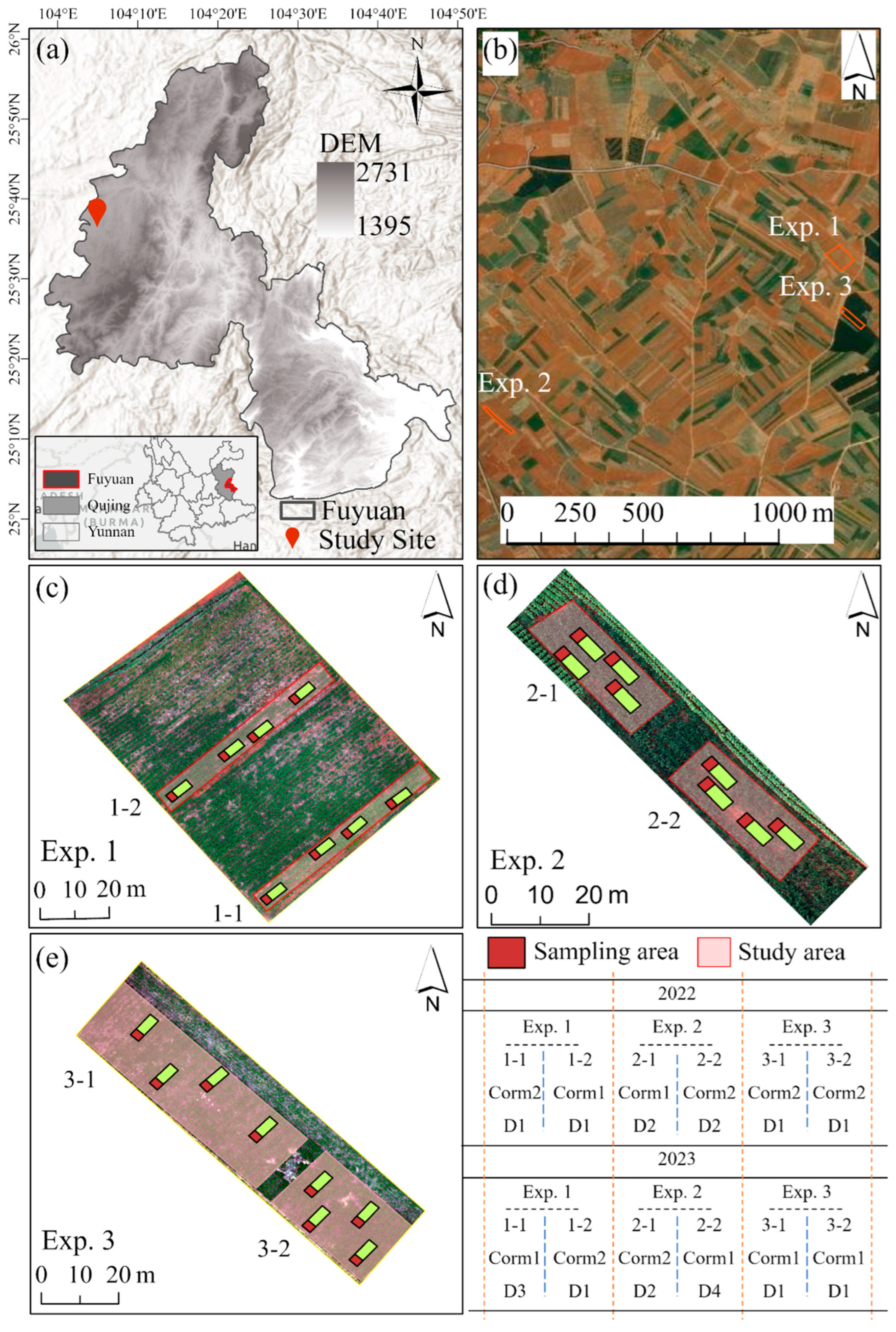
2.1. Experimental Design

The field experiments were conducted in Dazhaizikou Village, Fuyuan County, Qujing City, Yunnan Province (located at 25°36′25″ N, 104°4′55″ E, altitude: 2072 m), in 2022 and 2023 (Figure 1). Konjac is annually planted in April, with 0.896 t/hm² of organic fertilizer applied prior to planting and an additional 0.075 t/hm² of blended fertilizer (N:P:K = 15:15:15) applied before leaf emergence, as it prefers shaded conditions and is often intercropped with maize, which promotes its growth. The inclusion of one-year-old (corm 1) and two-year-old corms (corm 2), along with varying planting densities (D1: 7 plants/m², D2: 10 plants/m², D3: 9 plants/m², D4: 12 plants/m²) across three experimental plots (Exp. 1, Exp. 2, Exp. 3), was intended to enhance sample diversity, thereby better representing the range of conditions typically encountered in practical agricultural production. Overall, the study area consisted of 24 plots, each measuring 7 m × 2.5 m, and divided into two subplots. One subplot, measuring 2 m × 2.5 m, was designated for a destructive sampling area to obtain the measured AGB of Konjac, while the other subplot, measuring 5 m × 2.5 m, was used for a spectral sampling area to capture UAV-based spectral images during critical growth periods of Konjac.

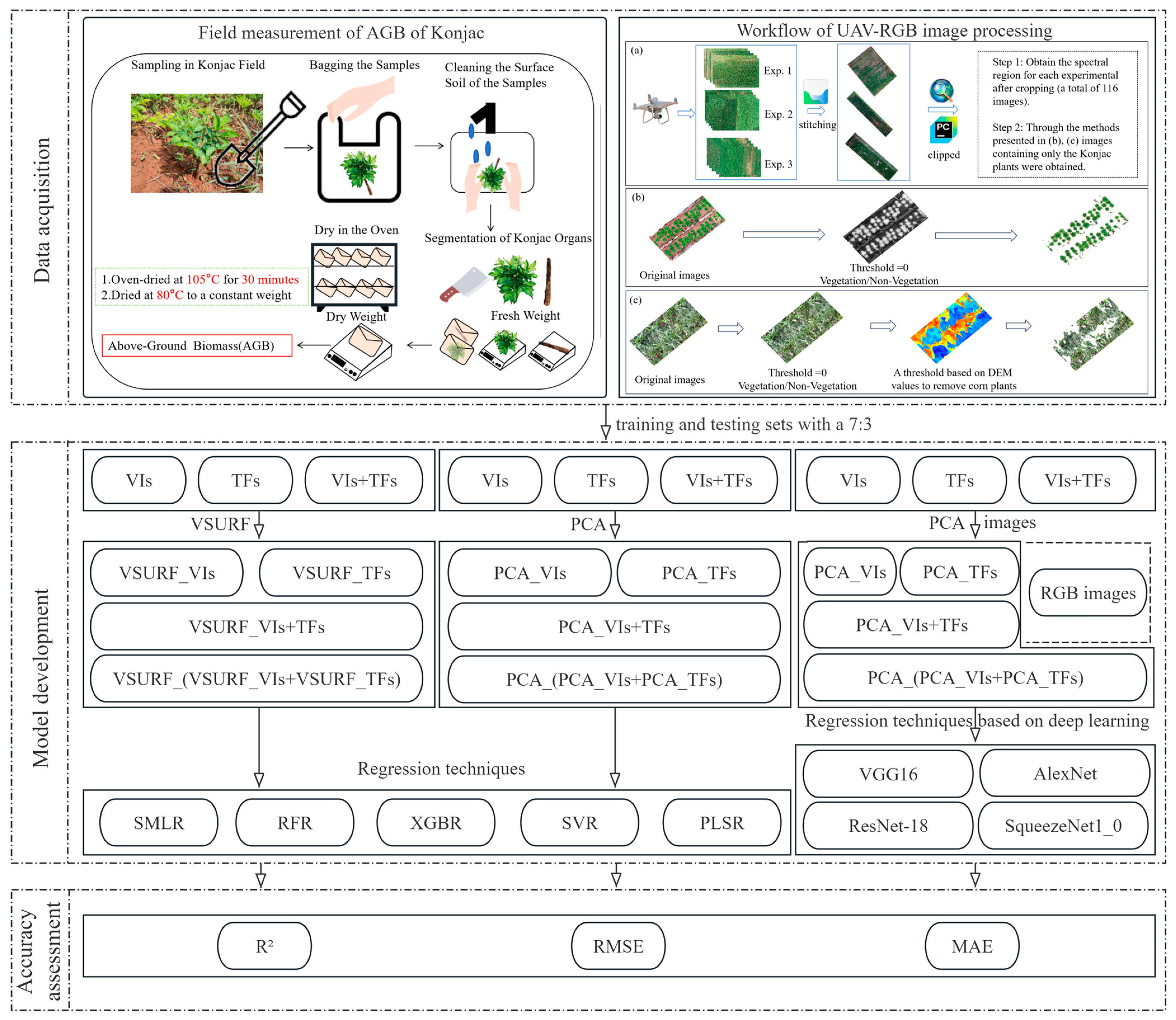
2.2. Data Acquisition

To acquire synchronized AGB and remote sensing data for Konjac, systematic field AGB measurements were conducted during critical growth stages, alongside the simultaneous acquisition of high-resolution RGB imagery using the UAV platform.

2.2.1. Field Measurement of Konjac AGB

The AGB of Konjac was collected at the critical growth stages indicated in

Table 2. The detailed information on the sampling date.

Date/Growth Period
Year	Seedling Stage (P1)	Tuber Initiation Stage (P2)	Tuber Enlargement Stage (P3)
2022	June 28	August 4	September 24
2023	July 28	August 17	-

Note: Delayed rainfall in the year 2023 postponed P1, while abundant rainfall during P2 supported normal growth, and climatic conditions during P3 resulted in the exclusion of this period from the dataset.

, specifically during the seedling stage (P1), tuber initiation stage (P2), and tuber enlargement stage (P3). A total of 116 Konjac AGB samples were collected from 24 plots over two years. However, due to variations in geographic location and extreme weather events, the dataset does not include the P3 period for Exp. 1 (from Subset 1-1 illustrated in Figure 1) in 2022, nor does it cover P3 periods for all plots in 2023. As shown in Figure 2, to obtain field AGB, three representative plants were selected from each of the 24 plots during each growth phase, with the selected plants chosen to represent the overall growth of their plots. Destructive sampling was conducted manually, with the samples immediately placed in plastic bags and transported to the laboratory, where the stem of Konjac was washed with clean water to remove surface soil. Subsequently, the stem and leaf organs of the Konjac plants were separated, and their fresh weights were recorded. The stem and leaf organs were then cut into small pieces, placed in envelopes, oven-dried at 105 °C for 30 min, and further dried at 80 °C until a constant weight was achieved. The AGB of the entire Konjac plant was calculated by summing the dry matter mass of the stem and leaf, with the average AGB of three plants per plot (in units of plant/hm²) used to determine the Konjac AGB for each plot, which is then adjusted based on the actual number of Konjac plants present in the plot.

2.2.2. Image Collection

This study employed the DJI Phantom 4 RTK (SZ DJI Technology Co., Shenzhen, China) to acquire high-resolution RGB images during three critical growth stages of Konjac. The DJI Phantom 4 RTK is an advanced UAV specifically designed for high-precision aerial mapping, surveying, and geospatial data collection. Equipped with a high-performance imaging system, the UAV incorporates a 1-inch 20-megapixel CMOS sensor, enabling the capture of detailed aerial imagery with a resolution of 5472 × 3648 pixels per image. The integration of RTK technology facilitates real-time differential corrections, achieving exceptional positional accuracy, with horizontal and vertical precision of 1 cm + 1 ppm and 1.5 cm + 1 ppm, respectively. The high precision and reliability of the DJI Phantom 4 RTK make it suitable for crop monitoring, yield estimation, and precision farming. To ensure the generation of high-precision point clouds and digital images, the flight altitude was set to 30 m, with a forward overlap of 80% and a side overlap of 70%. This parameter configuration ensures flight safety while enabling the acquisition of high-resolution imagery of Konjac, enhancing the quality and accuracy of orthomosaic generation in the image stitching process and mitigating errors caused by insufficient image overlap [29]. The camera ISO was set to 100, with the exposure adjusted based on weather conditions [13]. To minimize the impact of uneven sunlight on the quality and accuracy of RGB images captured by the UAV, flight campaigns were conducted under clear, stable weather conditions between 1:00 PM and 3:00 PM, following a consistent flight path throughout the critical growth stages of Konjac. In addition, the flight campaigns for the three experimental sites during each critical growth period of Konjac were conducted first, followed by field sampling on the same day.

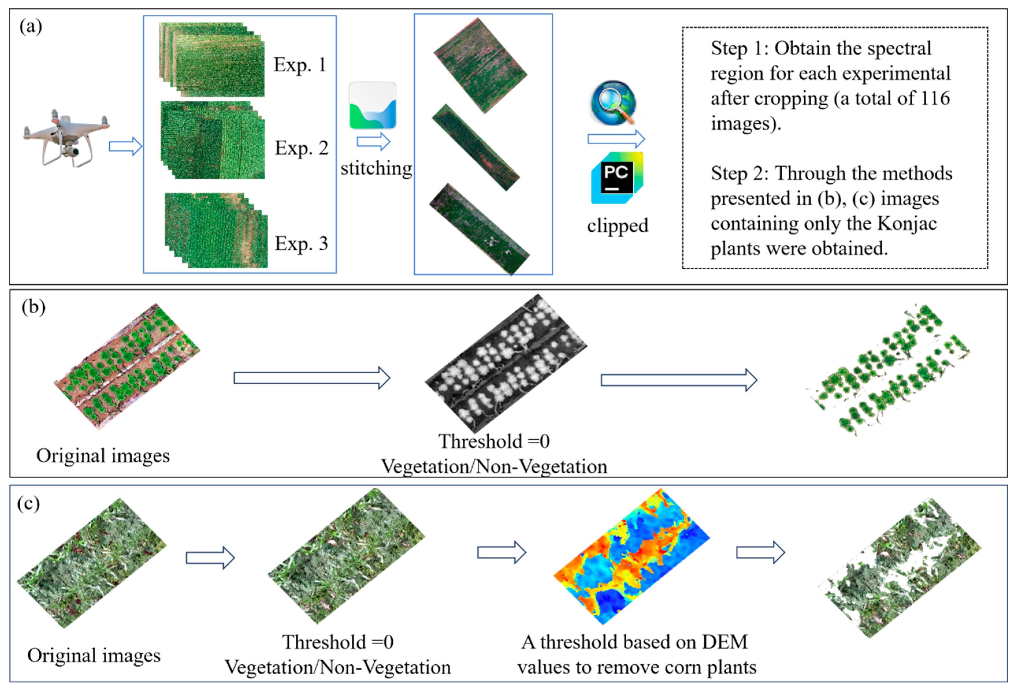
2.2.3. Image Processing

Orthomosaics and a Digital Elevation Model (DEM) of Konjac for each period were generated using Agisoft Metashape 1.8 software (Agisoft LLC, St. Petersburg, Russia) by stitching the original RGB images captured by the UAV for each period (Figure 3a). The software has been widely used in UAV image processing and is recognized in the field for its efficiency and reliability [13]. During the P1 (seedling) stage of Konjac, corn has not yet entered its developmental phase, and its plant height remains significantly lower than that of Konjac. Consequently, corn is rarely present in the acquired imagery, and its influence on the captured images can be considered negligible. However, during the P2 (tuber initiation) stage and P3 (tuber enlargement) stage, corn grows more rapidly than Konjac, and its plant height gradually surpasses that of Konjac. To eliminate the effects of soil and corn, as well as the portions of the image containing only Konjac plants, we first applied a threshold of 0 to the Modified Green Red Vegetation Index (MGRVI) (Table 3) image to remove non-vegetated areas (Figure 3b). Next, during the P2 and P3 stages, based on the height histogram distribution characteristics of Konjac and corn, we utilized the Otsu algorithm [30] to determine the optimal threshold for removing corn plants from the DEM. This process enabled the construction of a Konjac mask, which was subsequently used for extracting Konjac imagery (Figure 3c).

2.3. Feature Extraction

Feature extraction from UAV-acquired imagery includes the calculation of VIs and TF extraction, as well as feature selection and dimensionality reduction. These processes ensure the selection of optimal variables, reduce redundancy in the features, and contribute to more accurate AGB estimation.

2.3.1. Spectral Vegetation Calculation

VIs can reflect various characteristics of plants, such as growth status, coverage, and health, and are commonly used to estimate the AGB of different crops [31]. In this study, the Digital Number (DN) values of the R, G, and B channels, which quantitatively reflect the radiometric characteristics of the crops in the visible spectrum, were normalized using an equation (Equations (1)–(3)) to minimize the impact of illumination. The conversion from DN to reflectance was not performed due to the unavailability of spectral response functions. This study selected 13 representative VIs for Konjac AGB estimation (Table 3) based on relevant literature on estimating crop AGB using UAV-derived RGB images. The VI images were generated from the cropped spectral region, ensuring that the boundaries of the survey plots were excluded to avoid edge effects. The mean values extracted from these regions were used to represent individual survey plots.

$$r={\displaystyle \frac{R}{R+G+B}}$$

(1)

$$g={\displaystyle \frac{G}{R+G+B}}$$

(2)

$$b={\displaystyle \frac{B}{R+G+B}}$$

(3)

Table 3. The definition and description of Vegetation Indices.

VIs	Name	Formula	Reference
CIVE	Color Index of Vegetation	0.441r − 0.811g + 0.385b + 18.78745	[32]
EXB	Excess Blue Vegetation Index	1.4b − g	[33]
EXG	Excess Green Vegetation Index	2g − r − b	[33]
EXGR	Excess Green minus Excess Red Vegetation Index	3g − 2.4r − b	[33]
EXR	Excess Red Vegetation Index	1.4r − g	[34]
GLI	Green Leaf Index	(2g − r − b)/(2g + r + b)	[35]
GRRI	Green Red Ratio Index	r/g	[36]
MGRVI	Modified Green Red Vegetation Index	(g2 − r2)/(g2 + r2)	[37]
NDI	Normalized Difference Vegetation Index	(r − g)/(r + g + 0.01)	[38]
NGBDI	Normalized Green Blue Difference Index	(g − b)/(g + b)	[37]
NGRDI	Normalized Green Red Difference Index	(g − r)/(g + r)	[37]
RGBVI	Red Green Blue Vegetation Index	(g2 − br)/(g2 + br)	[37]
VARI	Visible Atmospherically Resistant Index	(g − r)/(g + r − b)	[39]

Table 3. The definition and description of Vegetation Indices.

VIs	Name	Formula	Reference
CIVE	Color Index of Vegetation	0.441r − 0.811g + 0.385b + 18.78745	[32]
EXB	Excess Blue Vegetation Index	1.4b − g	[33]
EXG	Excess Green Vegetation Index	2g − r − b	[33]
EXGR	Excess Green minus Excess Red Vegetation Index	3g − 2.4r − b	[33]
EXR	Excess Red Vegetation Index	1.4r − g	[34]
GLI	Green Leaf Index	(2g − r − b)/(2g + r + b)	[35]
GRRI	Green Red Ratio Index	r/g	[36]
MGRVI	Modified Green Red Vegetation Index	(g2 − r2)/(g2 + r2)	[37]
NDI	Normalized Difference Vegetation Index	(r − g)/(r + g + 0.01)	[38]
NGBDI	Normalized Green Blue Difference Index	(g − b)/(g + b)	[37]
NGRDI	Normalized Green Red Difference Index	(g − r)/(g + r)	[37]
RGBVI	Red Green Blue Vegetation Index	(g2 − br)/(g2 + br)	[37]
VARI	Visible Atmospherically Resistant Index	(g − r)/(g + r − b)	[39]

2.3.2. Texture Feature Extraction

The study utilizes 8 TFs based on Grayscale Co-occurrence Matrix (GLCM)—Mean (Mea), Variance (Var), Homogeneity (Hom), Contrast (Con), Dissimilarity (Dis), Entropy (Ent), Second Moment (Sec), and Correlation (Cor), as these are among the most commonly employed features in predictive models for crop AGB [2]. We set the GLCM displacement parameter to 3 pixels because the Konjac plants are relatively small, and their leaves exhibit an umbrella-shaped leaf blade characteristic, which helps capture the texture variation extending from the center to the outer edges of the leaves. This displacement also helps avoid excessive focus on noise, ensuring that the extracted TFs reflect biologically meaningful surface characteristics of the plant. In addition, we systematically evaluated the effects of the TF parameter window size (3 × 3, 5 × 5, 7 × 7, 9 × 9) and orientation (0°, 45°, 90°, 135°). To ensure clarity and conciseness, TFs were prefixed with ‘r.’, ‘g.’, or ‘b.’ to denote the texture extracted from the three channels based on GLCM (e.g., r.con refers to the contrast of the red band).

2.3.3. Feature Selection and Dimensionality Reduction

The combination of feature variables plays a crucial role in predicting Konjac AGB, but the inclusion of a large number of independent variables can increase model complexity and potentially lead to overfitting. Therefore, before feature combination and model construction, variable selection or dimensionality reduction is crucial for addressing the issue. Previous studies have demonstrated that VSURF and PCA methods can effectively perform variable selection or dimensionality reduction, leading to improved accuracy in biomass estimation [18,40]. Therefore, this study aims to evaluate the performance of variable selection using two distinct methods in estimating Konjac AGB. Specifically, PCA was applied separately to VIs (PCA_VIs), TFs (PCA_TFs), and their combination (Pacifists), as well as to the combination of PCA_VIs and PCA_TFs (PCA_(PCA_VIs+PCA_TFs)). Similarly, VSURF was applied separately to VIs (VSURF_VIs), TFs (VSURF_TFs), and their combination (VSURF_VIs+TFs), as well as the combination of VSURF_VIs and VSURF_TFs (VSURF_(VSURF_VIs+VSURF_TFs)), intending to optimize the predictive model by evaluating different variable selection and combination strategies. In the DL methods, PCA is applied to VI imagery, TF imagery, and their combination imagery.

2.4. Regression Techniques

To build a practical and reliable Konjac AGB model, this study assessed the performance of SMLR, ML, and DL-based regression techniques using high-resolution UAV-RGB imagery. Except for the DL-based regression method, which was implemented in Python 3.9, all other regression techniques were performed using the R programming language [41].

2.4.1. Stepwise Multiple Linear Regression

SMLR [42] dynamically introduces candidate predictor variables into the regression model one by one, thereby achieving feature selection, preventing overfitting, and reducing computational complexity in the process of building the linear model. Previous studies have demonstrated that SMLR achieves high accuracy in estimating wheat AGB [13], with an R² of 0.75 and an RMSE of 1.46 t/ha.

2.4.2. ML Regression Techniques

This study assessed the performance of four common ML regression algorithms (RFR, XGBR, PLSR, and SVR) for estimating the AGB of Konjac.

RFR, which was proposed by Breiman [43], is an ensemble learning method that estimates the target variable by constructing multiple decision trees, offering high estimation accuracy and robustness against overfitting. It has been demonstrated to achieve satisfactory accuracy (R² = 0.62) in estimating barley biomass [18].

XGBR, which was proposed by Chen and Guestrin [44], is a powerful model widely used in ML regression tasks due to its efficiency, accuracy, and strong ability to prevent overfitting. A recent study compared several regression models (SMLR, RFR, XGBR) and found that XGBR exhibited the highest estimation accuracy in monitoring maize AGB, with an R² of 0.81 and an RMSE of 0.27 t/ha [45].

PLSR, which was proposed by Wold et al. [46], was designed to reduce the dimensionality of the data by extracting latent variables, effectively preventing overfitting and enhancing the predictive performance of the model. Yue et al. [47] used Partial Least Squares Regression (PLSR) to estimate Winter Wheat Biomass, achieving an R² of 0.89, RMSE of 1.20 t/ha, and MAE of 0.90 t/ha.

SVR, which was proposed by Cortes and Vapnik [48], is capable of effectively handling the nonlinear relationships between independent and dependent variables and exhibits strong resistance to overfitting, making it widely applicable in various regression prediction tasks. For instance, Liang et al. [49] demonstrated that SVR achieved excellent accuracy in estimating the AGB of rubber plantations (R² = 0.752, RMSE = 28.72 t/ha).

Previous studies have shown that the hyperparameters of the ML regression technique can impact prediction accuracy [50]. Therefore, in this study, the hyperparameters for each regression model were directly set based on established guidelines and recommendations from prior work, and the specific parameter values are presented in

Table 4. The parameters of regression techniques.

Regression Techniques	Parameters
RFR	ntree = 500, nodesize = 1
XGBR	max_depth = 6, eta = 0.01
PLSR	-
SVR	kernel = “radial”

.

2.4.3. DL-Based Regression Techniques

DL methods can automatically extract meaningful features from images by learning convolutional filters, thereby replacing the traditional manual feature extraction process. DL methods typically require large datasets for training. For example, Jia et al. [51] employed a DL model for plant detection, utilizing over 1000 images. However, in biomass estimation tasks, due to the costs associated with sample acquisition, the number of plots, and time constraints, it is often not feasible to achieve such a scale of training. This study employs the following networks from Pytorch: AlexNet, ResNet-18, SqueezeNet1_0, and VGG16. To adapt the model for regression tasks, the architecture of the final fully connected layer was modified. All experiments were conducted using the Adam optimizer [25] with a fixed learning rate of 0.0001, and the early stopping mechanism was set to 50 epochs to determine the final epoch. Pre-trained models from torchvision were used for all models [52]. Castro et al. [53] found that when estimating grass biomass using a small sample size with DL, the augmented samples improved prediction accuracy. Therefore, data augmentation was applied to all training data in this study to enhance the model’s performance (including horizontal flip, vertical flip, and rotation). Before training the model, the images were normalized to the range [0, 1] to enhance the stability of the DL model during training [54]. The network input consisted of images resized to 224 × 224 pixels and their corresponding AGB target values. Although previous studies have demonstrated good accuracy (R² = 0.94, RMSE = 62 g/m²) in estimating pasture biomass using RGB images combined with DL [25], there is limited research on using VIs and texture feature images with DL for biomass estimation. These datasets often contain many correlated bands or features, and PCA helps reduce the number of input features while retaining the majority of the important information. In this study, PCA is applied to the individual VIs and texture images, as well as their combinations, which may offer alternative perspectives and enhanced information, potentially improving biomass estimation performance. Therefore, the input images consist not only of RGB images but also PCA-based images. For each of these PCA-based image sets, the first three principal components were selected to correspond to the three channels of the RGB images. The processor used is an Intel(R) Core(TM) i9-14900HX, with a graphics card of NVIDIA GeForce RTX 4070 and 64 GB of RAM.

2.5. Accuracy Assessment

The statistical analysis process following data collection is shown in Figure 4. The data are divided based on different collection dates and plots to ensure an even distribution, preventing substantial discrepancies. To ensure reproducibility, a random seed was set during the data splitting. The data, comprising a total of 116 samples, are divided into training and testing sets in a 7:3 ratio [49], with 81 samples in the training set and 35 samples in the testing set. In DL, the augmented training set includes 162 samples. The performance of five ML algorithms was systematically evaluated using different variable groups derived from PCA and VSURF. In the DL approach, we also compared the performance of four DL methods using RGB imagery and images derived from different variable sets obtained through PCA. Finally, the coefficient of determination (R²), Root Mean Square Error (RMSE), and Mean Absolute Error (MAE) were used to evaluate the performance of the model in estimating the Konjac AGB. A detailed summary of the statistics is provided in

Table 5. The statistics of the field-measured Konjac AGB (t/hm²) for the training and testing datasets.

Dataset	Min	Mean	Max	Standard Deviation	Coefficient of Variation (%)
Training	0.03	0.56	1.46	0.39	68.63
Testing	0.02	0.60	1.46	0.40	66.93
All	0.02	0.57	1.46	0.39	67.86

.

3. Results

This study systematically investigates the correlation between AGB and multiple UAV-derived variables while performing a comprehensive evaluation of several regression approaches, including SMLR, diverse ML regression algorithms, and DL-based regression methods for AGB estimation.

3.1. Correlation Analysis Between AGB and UAV-Derived Variables

To determine the most significant features derived from VIs and TFs for AGB estimation and to elucidate their interrelationships, a comprehensive correlation analysis was conducted between AGB and the extracted features from both VIs and TFs. Furthermore, to enhance feature selection efficiency and mitigate the impact of feature redundancy, an additional correlation analysis was performed among the optimized feature variables.

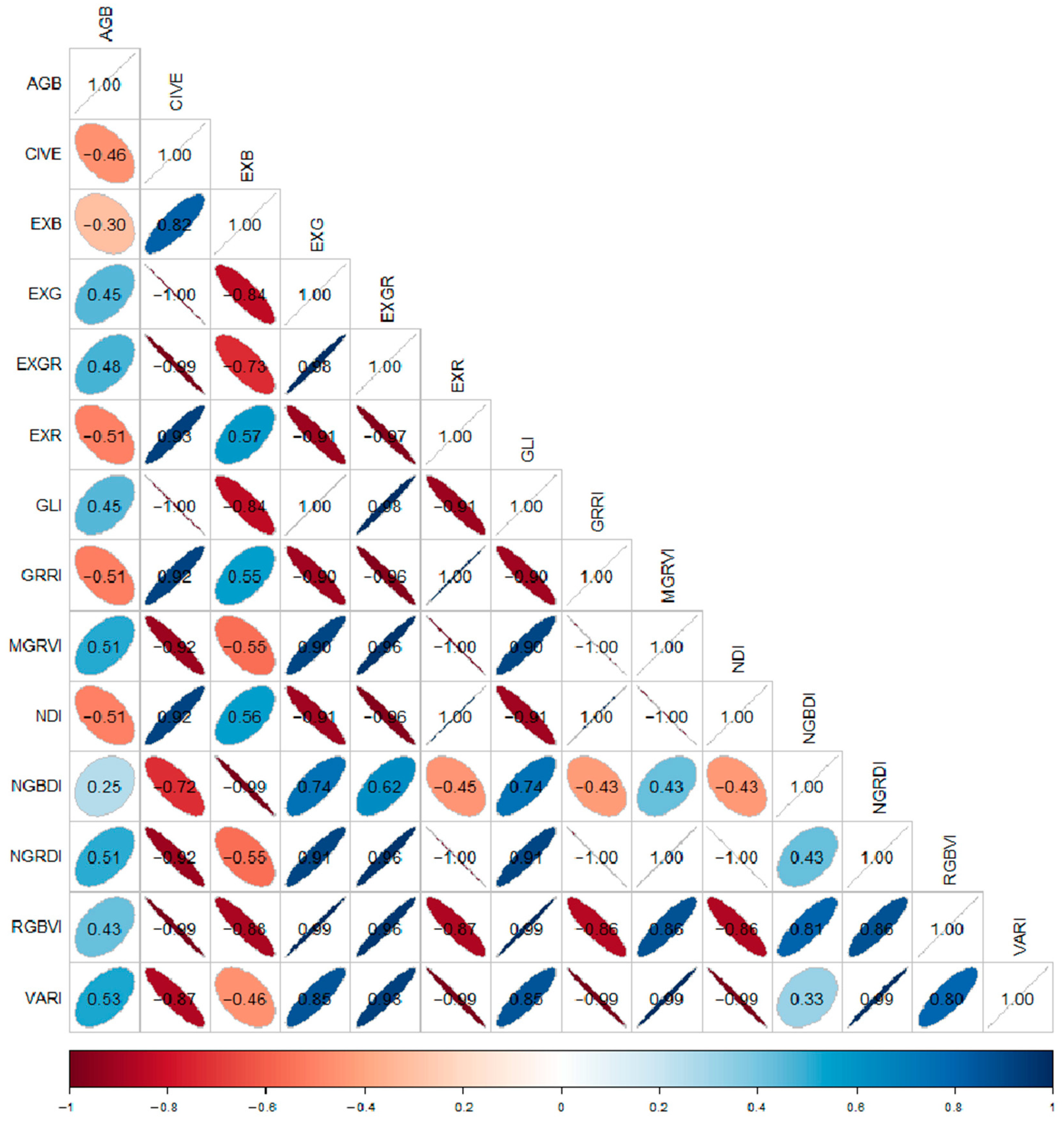
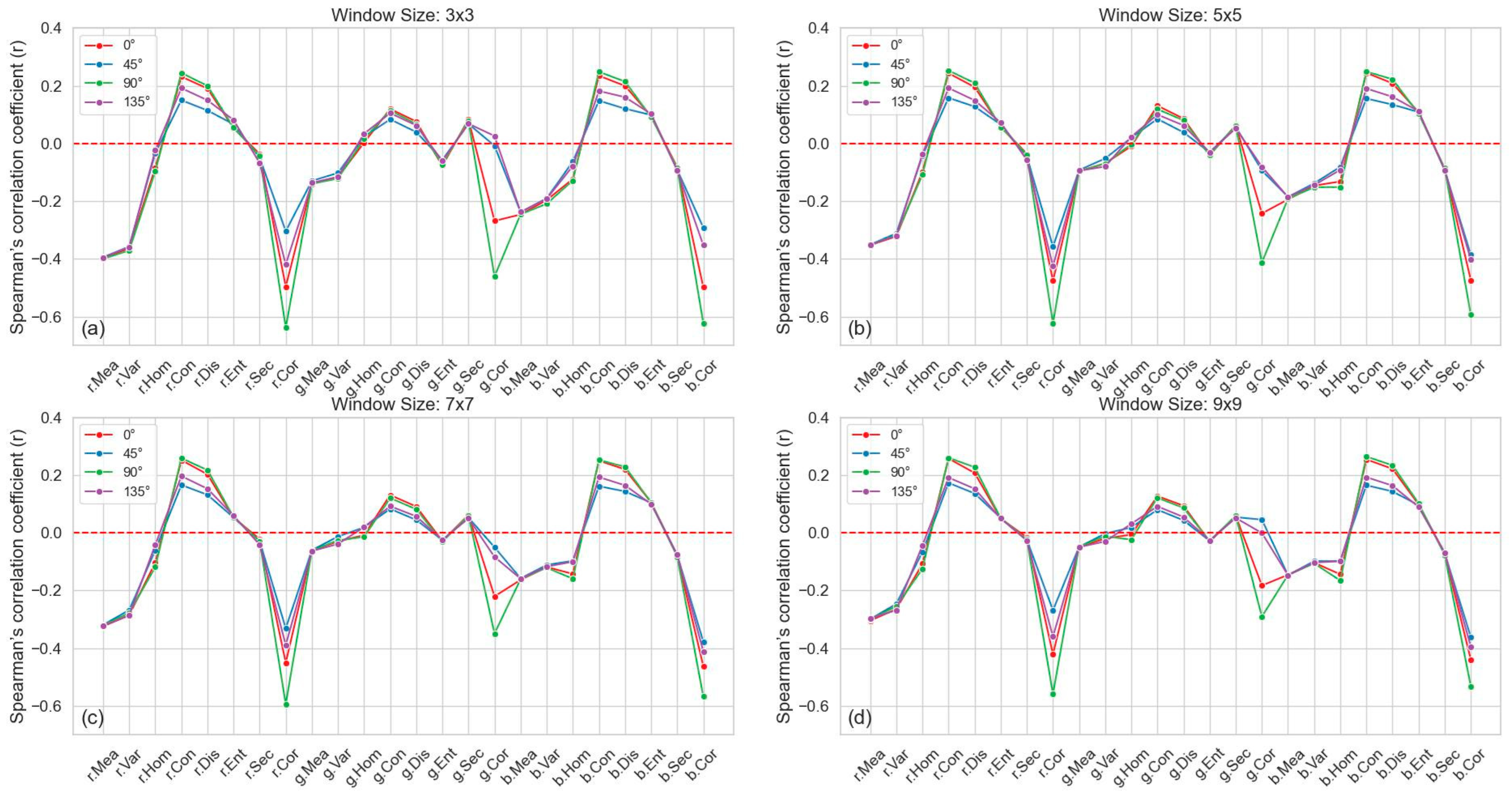
3.1.1. Correlation Analysis of AGB with VIs and TFs

Figure 5 demonstrates Spearman’s correlation coefficient (r) between the measured AGB of Konjac and 13 VIs used in this study. The results show a significant correlation between the VIs and AGB, particularly with the highest positive correlation between VARI and AGB (r = 0.53). These 13 VIs demonstrate a strong positive or negative correlation, with (|r|) values equal to 1 (CIVE vs. EXG, GLI; EXG vs. GLI; EXR vs. GRRI, MGRVI, NDI, NGRD; GRRI vs. MGRVI, NDI, NGRDI, VARI, MGRVI vs. NDI, NGRDI; NDI vs. NGRDI).

To determine the optimal GLCM parameters for TF extraction from UAV-based RGB images, a systematic evaluation was conducted to assess the impact of different directions and window sizes on Spearman’s correlation coefficient (r) with the AGB of Konjac. As shown in Figure 6, the correlation between TFs and the AGB of Konjac varies across different directions and window sizes. The results demonstrate that the TFs exhibit minimal sensitivity to changes in window size while showing a strong dependence on orientation. Specifically, the optimal correlation between the TFs and the AGB of Konjac was achieved at an orientation of 90° and a window size of 3 × 3. Thus, this study adopts GLCM parameters with a 3 × 3 window size and a 90° orientation. The correlation-based features, including b.cor, g.cor, and r.cor, exhibit the highest influence on AGB correlation, with their relationship being most affected by orientation settings.

Figure 7 shows Spearman’s correlation coefficients (r) between the measured AGB of Konjac and the 24 TFs, calculated with a 3 × 3 window size and a 90° orientation. The analysis revealed that AGB is most strongly negatively correlated with the r.cor texture feature (r = −0.64) and most weakly positively correlated with the g.hom texture feature (r = 0.02). Among the twenty-four TFs, eight exhibited highly positive correlations, with the (|r|) values reaching 1 (r.Cor vs. r.Sec; g.Ent vs. g.Sec; b.Con vs. b.Dis; b.Ent vs. b.Sec).

3.1.2. Correlation Analysis Between AGB and Feature-Optimized Variables

To optimize model performance and minimize overfitting, we employed VSURF to identify the most influential variables. VSURF was applied separately to the VIs, TFs, their combination, and the variables selected from individual VSURF analyses of both the VIs and TFs. The results of the selected variable groups are presented in

Table 6. Different feature groups were selected to estimate Konjac AGB using VSURF.

Variable Name	Parameters
VSURF_VIs	VARI, GRRI, RGBVI
VSURF_TFs	r.Cor, b.Cor, r.Con, r.Mea, b.Con, g.Sec, b.Sec
VSURF_(VIs+TFs)	VARI, r.Cor, GRRI, MGRVI, b.Cor, RGBVI, CIVE, r.Con, g.Var, g.Mea
VSURF_(VSURF_VIs+VSURF_TFs)	VARI, GRRI, r.Cor, b.Cor, RGBVI, r.Con

Note: VSURF_VIs represents the optimized variables set derived from VIs using VSURF. VSURF_TFs represents the optimized variables set derived from TFs using VSURF. VSURF_(VIs+TFs) represents the optimized variables set derived from VIs and TFs using VSURF. VSURF_(VSURF_VIs+VSURF_TFs) represents the optimized variables set derived from VSURF_VIs and VSURF_TFs using VSURF.

. The results indicate that VSURF effectively reduces redundant information while retaining the most informative and relevant features. Both VSURF_VIs+TFs and VSURF_(VSURF_VIs+VSURF_TFs) preserve a richer set of feature information. Similarly, we performed PCA separately on the VIs, the TFs, their combination, and the principal components obtained from the individual PCA of both the VIs and TFs. This study utilized the top three principal components, as illustrated in the PCA analysis presented in Figure 8, accounting for the majority of the significant information and explaining over 70% of the variance.

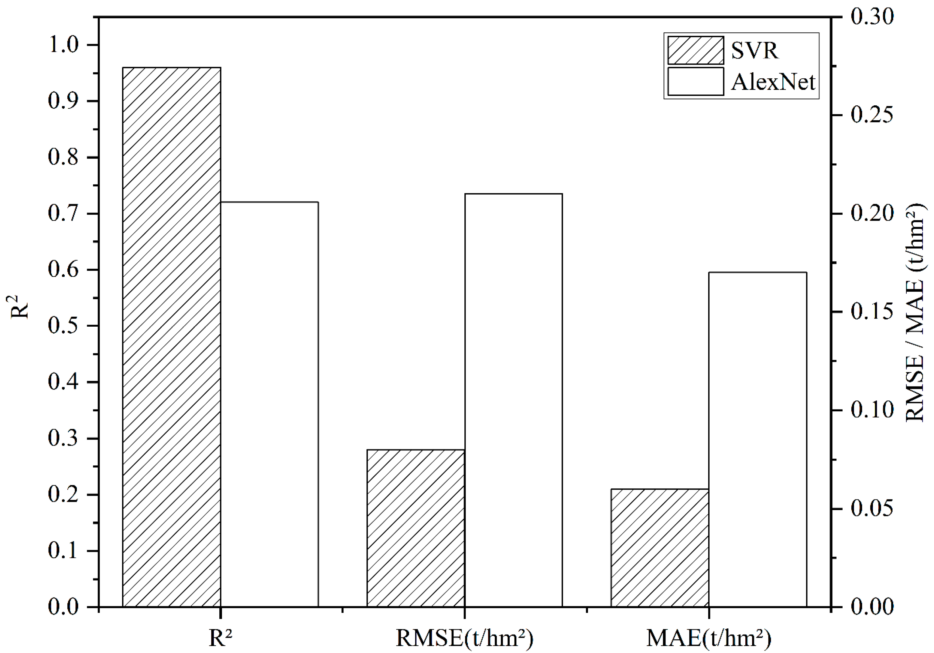
3.2. The Performance of SMLR and ML Regression Techniques Using Selected Variables

The variable groups selected using VSURF were evaluated using five regression techniques (SMLR, RFR, XGBR, PLSR, SVR) to identify the optimal model for estimating Konjac AGB (

Table 7. Different selected variable groups using VSURF for estimating Konjac AGB.

Method	Assessment Metrics	VSURF_VIs	VSURF_TFs	VSURF_VIs+TFs	VSURF_(VSURF_VIs+VSURF_TFs)
SMLR	R2	0.22	0.41	0.60	0.44
	RMSE (t/hm2)	0.35	0.30	0.25	0.30
	MAE (t/hm2)	0.27	0.25	0.20	0.23
RFR	R2	0.50	0.46	0.64	0.62
	RMSE (t/hm2)	0.28	0.29	0.24	0.24
	MAE (t/hm2)	0.20	0.20	0.18	0.18
XGBR	R2	0.45	0.42	0.51	0.52
	RMSE (t/hm2)	0.29	0.30	0.27	0.27
	MAE (t/hm2)	0.22	0.22	0.22	0.21
PLSR	R2	0.24	0.40	0.60	0.44
	RMSE (t/hm2)	0.34	0.31	0.25	0.29
	MAE (t/hm2)	0.26	0.24	0.2	0.23
SVR	R2	0.42	0.31	0.57	0.53
	RMSE (t/hm2)	0.30	0.33	0.26	0.27
	MAE (t/hm2)	0.21	0.22	0.20	0.19

). When it comes to feature variable optimization, the variable optimized combination (VSURF_VIs+TFs, VSURF_(VSURF_VIs+VSURF_TFs)) of VIs and TFs using VSURF outperformed the use of VSURF_VIs or VSURF_TFs alone across different regression techniques. Among the five regression models, ML models outperformed SMLR in estimating Konjac AGB. Specifically, the RFR combined with the selected variables of VSURF_VIs+TFs exhibited the highest accuracy, with R² of 0.64, RMSE of 0.24 t/hm², and MAE of 0.18 t/hm². In contrast, SMLR performed the worst with the VSURF_VIs, showing R² of 0.22, RMSE of 0.35 t/hm², and MAE of 0.27 t/hm².

The study utilized PCA for the dimensionality reduction of variables and evaluated different feature combinations using five regression techniques to establish the optimal model for estimating Konjac AGB. Figure 9 demonstrates that the feature combination of PCA_(PCA_VIs +PCA_TFs) achieved outstanding performance across all five regression techniques. Moreover, the feature combination (PCA_(PCA_VIs +PCA_TFs)) coupled with SVR obtained the highest estimation accuracy with R² of 0.96, RMSE of 0.08 t/hm², and MAE of 0.06 t/hm². In contrast, the variable group of PCA_VIs+TFs performed the worst with the SMLR, showing R² of 0.27, RMSE of 0.34 t/hm², and MAE of 0.25 t/hm².

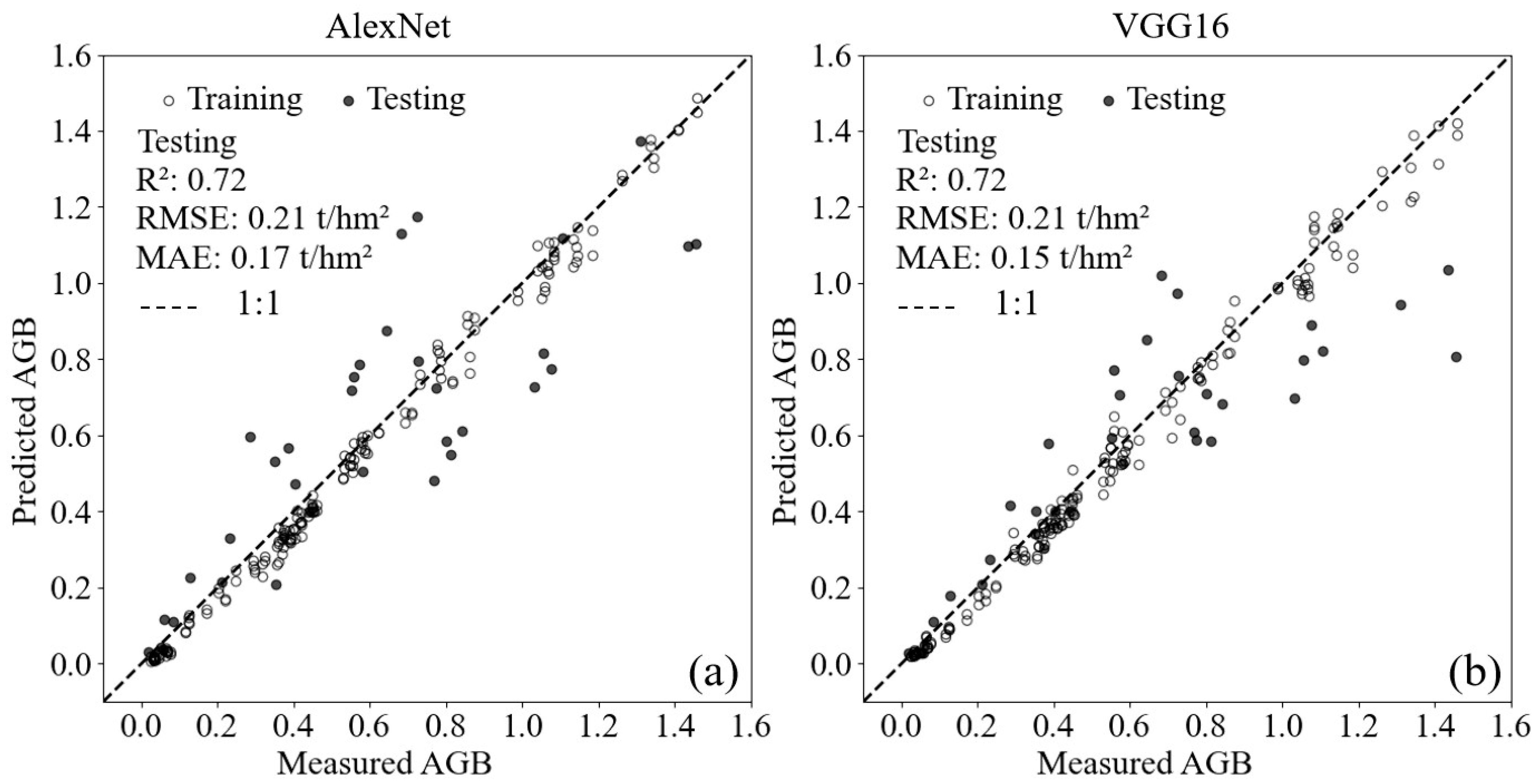
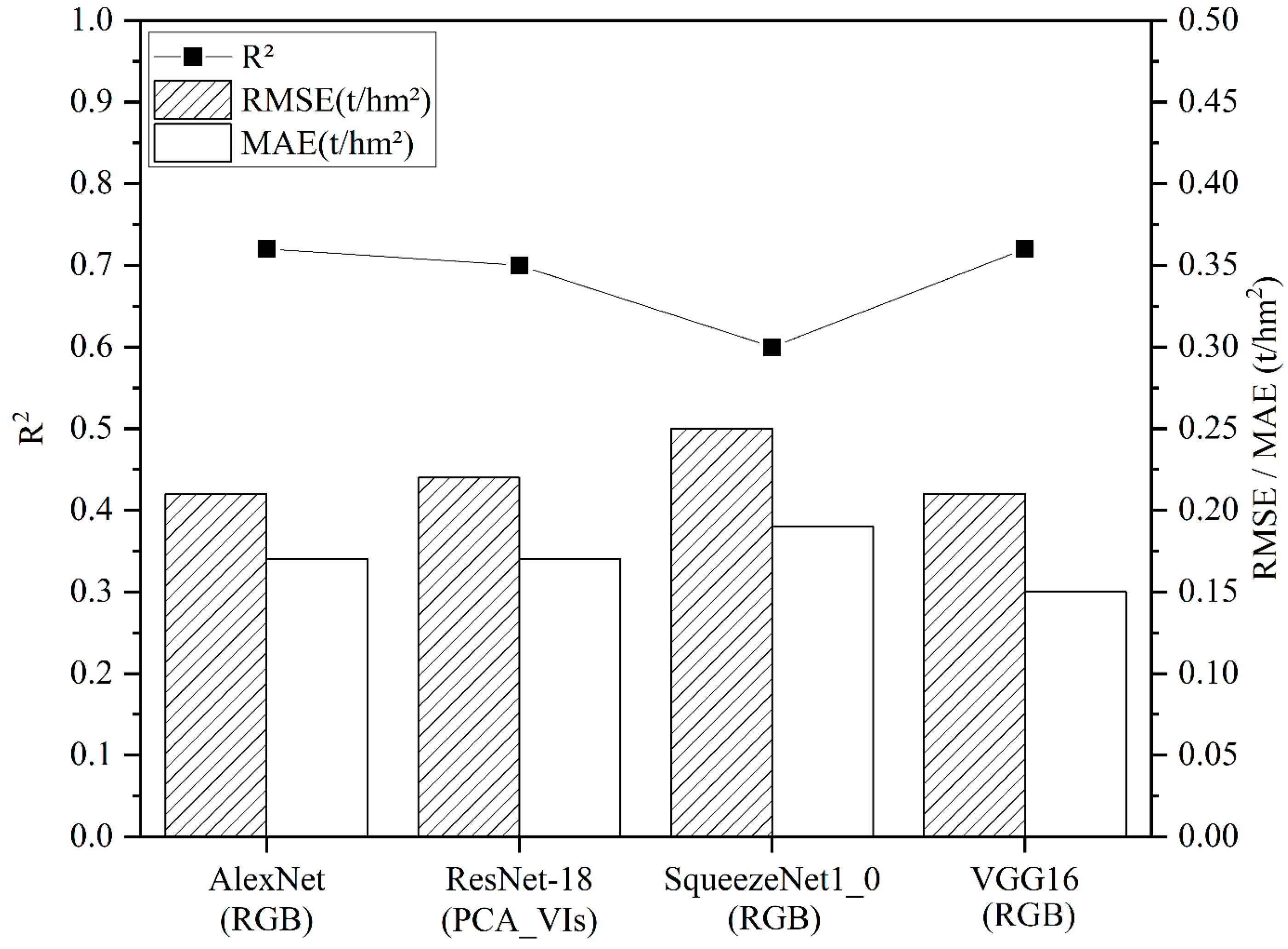
3.3. The Effectiveness of DL-Based Network Models Utilizing Selected Variables

This study systematically evaluated the performance of different input image groups in predicting Konjac AGB across four DL network models (AlexNet, ResNet-18, SqueezeNet1_0, VGG16). Figure S1 in Supplementary Materials demonstrates that among the four DL network models, the input RGB images resulted in the highest accuracy, except for the ResNet-18 model. Specifically, both the AlexNet and VGG16 networks demonstrated high accuracy in AGB prediction using RGB images, with R² of 0.72 and RMSE of 0.21 t/hm². However, VGG16 exhibited slightly better performance than AlexNet, as its MAE was 0.02 t/hm² lower (Figure 10).

4. Discussion

This study systematically examines the impact of GLCM parameters on their correlation with Konjac AGB estimation, with particular emphasis on how optimal parameter selection can significantly improve the correlation in AGB estimation. The investigation further elucidates the distinctive advantages of ML approaches, specifically highlighting their robustness in handling limited sample sizes and complex computational tasks. A comparative analysis was subsequently performed between DL methodologies utilizing RGB imagery and PCA-based imagery, demonstrating the superior feature extraction capabilities and predictive performance of DL models with RGB inputs. The study concludes with a comprehensive evaluation of ML and DL approaches, critically assessing their respective potentials and limitations in practical agricultural applications and proposing methodological recommendations and future research directions for improved AGB estimation in Konjac cultivation.

4.1. The Influence of GLCM Parameters on the Correlation with Konjac AGB

Our results indicate that the orientation of GLCM parameters has a more sensitive impact on the Spearman correlation with Konjac AGB than the window size (Figure 6). This is inconsistent with the findings of Liu et al. [2], who reported that the direction and window size of GLCM texture parameters have no significant impact on the correlation with potato AGB. This difference may be attributed to the distinct plant traits between the two species, with Konjac exhibiting more pronounced texture variations at specific directions or window sizes due to its leaves being concentrated around the central stem, whereas potato has leaves distributed along the stem, resulting in less directional texture variation. Among these TFs, b.cor, g.cor, and r.cor exhibit the greatest sensitivity to directional changes, meaning their correlation with AGB varies significantly. This can be explained by the fact that the umbrella-shaped leaf blade of Konjac typically features a denser canopy around the central stem, which results in significant texture variations depending on the observation direction [55]. When the plant structure is viewed from different orientations, these dense arrangements cause changes in the spatial correlation between pixels. This directional variation enhances the sensitivity of the correlation-based features (b.cor, g.cor, r.cor) to changes in the observation orientation. The results of this study indicate that when the window size is 3 × 3 and the orientation is 90°, the TFs show the best correlation with the AGB of Konjac. This is consistent with the findings of Niu et al. [56], who observed that a 90° orientation yielded the best performance in estimating the fresh and dry biomass of maize. The intercropping of Konjac with maize, with rows planted in the same direction, better reflects vegetation distribution, arrangement, and morphological features along the 90° direction.

4.2. Advantages of ML Techniques

In this study, the variable selection methods PCA and VSURF were compared across five different regression techniques (SMLR, RFR, XGBR, PLSR, SVR) to estimate the AGB of Konjac. The results indicate that the predictive performance of ML models outperforms SMLR. This can be attributed to the fact that remote sensing variables do not exhibit a simple linear relationship with Konjac AGB. While SMLR is effective for simple linear regression problems, ML models are better suited to handle more complex tasks [49]. Furthermore, among the various feature combinations evaluated using the VSURF method, the combination of VSURF_VIs+TFs with RFR achieved the best performance (R² = 0.64, RMSE = 0.24 t/hm², MAE = 0.18 t/hm²). This finding is consistent with the results of Wengert et al. [18], who applied VSURF for variable selection in RFR to predict barley whole crop biomass, achieving an R² of 0.60. As VSURF is a feature selection method based on random RFR, their combination enables more efficient identification and retention of significant variables during the feature selection process, thereby improving the overall accuracy of the model. Figure 11 illustrates the performance of various feature selection methods, including VSURF and PCA. Compared to the VSURF-based models, the PCA-based approach, particularly using PCA_(PCA_VIs+PCA_TFs), demonstrated superior performance, with SVR for estimating the AGB of Konjac achieving R² of 0.96, RMSE of 0.08 t/hm², and MAE of 0.06 t/hm². Previous research has shown that VSURF may not yield as accurate results as PCA-based variable selection [57]. This implies that the dimensionality reduction performed by PCA may have better alleviated the inherent redundancy and collinearity in the data, which is particularly advantageous for models such as SVR, which are more susceptible to these issues. Previous studies have shown that combining PCA with RFR for estimating wheat AGB outperformed other ML models [19]. However, in our study, the PCA-based approach with RFR yielded inferior performance compared to SVR, which may be attributed to the differences in traits between the two crops, as such differences could affect the efficacy of PCA in feature selection and the performance of the model. The superior performance of the PCA-based method in this case highlights the potential advantages of dimensionality reduction when applied to models that benefit from a simpler, more compact feature space [58].

4.3. Advantages of DL Methods Combined with RGB Imagery for Konjac AGB Estimation Compared to PCA-Based Images

Our results demonstrate that, when estimating Konjac AGB using DL methods, RGB images consistently achieved the highest accuracy across all models, except for the ResNet-18 network, where the PCA-based vegetation index images yielded superior performance (Figure 12). This may be attributed to the fact that RGB images contain rich color information, which can effectively capture features related to plant growth [22], in contrast to PCA-based images, which may lose some of this crucial information. In contrast, PCA-based vegetation index images may, in specific instances, enhance feature extraction for the ResNet-18 model. Among these DL models, AlexNet and VGG16 demonstrated the best performance, which is consistent with recent studies that reported favorable results when using the AlexNet network for AGB estimation in rubber plantations [53]. Although the accuracy of VGG16 slightly outperforms that of the AlexNet network in this study, the training time for VGG16 is approximately 120 min, while the AlexNet network, along with other networks, requires only about 2 min (

Table 8. Accuracy assessment for estimating the AGB of Konjac using four DL models.

DL	Images	R2	RMSE (t/hm2)	MAE (t/hm2)	Training Time
AlexNet	RGB	0.72	0.21	0.17	2 min
ResNet-18	PCA_VIs	0.70	0.22	0.17	2 min
SqueezeNet1_0	RGB	0.6	0.25	0.19	4 min
VGG16	RGB	0.72	0.21	0.15	120 min

). Given the lower complexity of the AlexNet network compared to VGG16 [59], it is better suited for the dataset used in this study. This suggests that, despite VGG16 having higher accuracy, AlexNet may be more advantageous in terms of computational efficiency, especially for large-scale or time-sensitive applications.

4.4. Potential Applications and Limitations

This study developed an AGB estimation model for Konjac utilizing high-resolution RGB imagery obtained from the DJI Phantom 4 RTK UAV platform. The model demonstrated promising estimation accuracy, highlighting its applicability for precise AGB assessment. In alignment with the findings of Liang et al. [49], the consumer-grade DJI Phantom 4 RTK exhibits great potential for biomass estimation in agricultural and forestry applications. Among the regression techniques evaluated, SVR combined with the variable integration of PCA_(PCA_VIs+PCA_TFs) derived from UAV-based RGB imagery using PCA for estimating the AGB of Konjac achieved the best performance compared to RFR, XGBR, PLSR, and SMLR. Previous studies have also demonstrated that SVR exhibits high accuracy, even under small sample conditions [49]. In addition, the performance of the AlexNet model in the DL approaches was inferior to that of the SVR model in the ML approaches (Figure 13), which may be attributed to the relatively small sample size (116 samples). Consistent with these findings, Tamiminia et al. [60] demonstrated in their comprehensive investigation of shrub willow biomass estimation that ML approaches exhibited superior performance compared to DL methodologies, primarily attributed to the substantial training data requirements inherent to DL model architectures. However, a recent study by Tan et al. [57] demonstrated that DL methods outperformed ML in estimating AGB in rubber plantations despite using a similar small sample size (80 samples). The difference between the two studies is likely attributed to the greater variability in Konjac images across different plots in this study, primarily due to variations in planting and acquisition times. In contrast, the variability between plots in rubber plantations is comparatively smaller, which suggests that DL models may require fewer samples than Konjac images to achieve optimal performance. Therefore, future research will focus on expanding the sample size by incorporating additional Konjac samples, which is expected to enhance the performance of the DL model. Furthermore, the imagery used in this study only included Konjac plants, with corn plants being removed based on DEM threshold values due to the significant height difference between corn and Konjac plants. However, in other planting areas, the height of corn and Konjac plants may be similar, which could limit the effectiveness of the method used in this study for removing corn plants. Given the morphological differences between Konjac and corn, future research will explore the use of DL methods to identify Konjac plants in order to retain the portions of the imagery corresponding to Konjac plants.

5. Conclusions

This study systematically assessed the performance of two variable selection methods (PCA and VSURF) for estimating Konjac AGB using regression techniques (SMLR, ML, DL) with UAV-based RGB imagery that included only Konjac plants. The results indicated that SVR combined with the integration (PCA_(PCA_VIs+PCA_TFs)) of selected variables from PCA-based VIs and PCA-based TFs using PCA produced the most accurate estimations (R² = 0.96, RMSE = 0.08 t/hm², MAE = 0.06 t/hm²). This methodological framework significantly enhances AGB estimation accuracy by effectively reducing the dimensionality of input features while preserving critical information in combination with the robust SVR algorithm. In contrast, the AlexNet network using RGB imagery in DL methods produced moderate accuracy with R² of 0.72, RMSE of 0.21 t/hm², and MAE of 0.17 t/hm². Our findings suggest that SVR integrated with the combination of VIs and TFs derived from UAV RGB imagery using PCA improved the estimation accuracy of Konjac AGB, making it more suitable for small sample estimation than DL methods. This study proposes a method for estimating Konjac AGB by combining imagery that exclusively contains Konjac plants with PCA-selected variables and the SVR technique, providing new insights and potential application directions for monitoring the growth status of other crops. Furthermore, our research highlights the considerable potential of the consumer-grade DJI Phantom 4 RTK in crop AGB estimation, underscoring its utility as a cost-effective and efficient tool for precision agriculture. Future research will focus on expanding the sample size of Konjac to improve model robustness and enhance its generalization capabilities across diverse cultivation conditions. Following this methodological enhancement, subsequent investigations will systematically evaluate the efficacy of DL approaches for AGB estimation in Konjac, incorporating state-of-the-art DL architectures and advanced computational frameworks to optimize predictive performance.

References

1. Zhuo, W.; Huang, J.; Li, L.; Zhang, X.; Ma, H.; Gao, X.; Huang, H.; Xu, B.; Xiao, X. Assimilating soil moisture retrieved from Sentinel-1 and Sentinel-2 data into WOFOST model to improve winter wheat yield estimation. Remote Sens. 2019, 11, 1618. [Google Scholar] [CrossRef]
2. Liu, Y.; Feng, H.; Yue, J.; Jin, X.; Li, Z.; Yang, G. Estimation of potato above-ground biomass based on unmanned aerial vehicle red-green-blue images with different texture features and crop height. Front. Plant Sci. 2022, 13, 938216. [Google Scholar] [CrossRef] [PubMed]
3. Kumar, A.; Tewari, S.; Singh, H.; Kumar, P.; Kumar, N.; Bisht, S.; Kushwaha, S.; Tamta, N.; Kaushal, R. Biomass accumulation and carbon stocks in different agroforestry system prevalent in Himalayan foothills, India. Curr. Sci. 2021, 120, 1083–1088. [Google Scholar] [CrossRef]
4. Fu, Y.; Tan, H.; Kou, W.; Xu, W.; Wang, H.; Lu, N. Estimation of Rubber Plantation Biomass Based on Variable Optimization from Sentinel-2 Remote Sensing Imagery. Forests 2024, 15, 900. [Google Scholar] [CrossRef]
5. Wang, L.; Jia, M.; Yin, D.; Tian, J. A review of remote sensing for mangrove forests: 1956–2018. Remote Sens. Environ. 2019, 231, 111223. [Google Scholar] [CrossRef]
6. Duan, B.; Fang, S.; Gong, Y.; Peng, Y.; Wu, X.; Zhu, R. Remote estimation of grain yield based on UAV data in different rice cultivars under contrasting climatic zone. Field Crops Res. 2021, 267, 108148. [Google Scholar] [CrossRef]
7. Liu, Y.; Feng, H.; Yue, J.; Jin, X.; Fan, Y.; Chen, R.; Bian, M.; Ma, Y.; Li, J.; Xu, B. Improving potato AGB estimation to mitigate phenological stage impacts through depth features from hyperspectral data. Comput. Electron. Agric. 2024, 219, 108808. [Google Scholar] [CrossRef]
8. Guo, Y.; He, J.; Zhang, H.; Shi, Z.; Wei, P.; Jing, Y.; Yang, X.; Zhang, Y.; Wang, L.; Zheng, G. Improvement of Winter Wheat Aboveground Biomass Estimation Using Digital Surface Model Information Extracted from Unmanned-Aerial-Vehicle-Based Multispectral Images. Agriculture 2024, 14, 378. [Google Scholar] [CrossRef]
9. Liu, T.; Yang, T.; Zhu, S.; Mou, N.; Zhang, W.; Wu, W.; Zhao, Y.; Yao, Z.; Sun, J.; Chen, C. Estimation of wheat biomass based on phenological identification and spectral response. Comput. Electron. Agric. 2024, 222, 109076. [Google Scholar] [CrossRef]
10. Yang, H.; Li, F.; Wang, W.; Yu, K. Estimating Above-Ground Biomass of Potato Using Random Forest and Optimized Hyperspectral Indices. Remote Sens. 2021, 13, 2339. [Google Scholar] [CrossRef]
11. Wang, F.; Yang, M.; Ma, L.; Zhang, T.; Qin, W.; Li, W.; Zhang, Y.; Sun, Z.; Wang, Z.; Li, F. Estimation of above-ground biomass of winter wheat based on consumer-grade multi-spectral UAV. Remote Sens. 2022, 14, 1251. [Google Scholar] [CrossRef]
12. Song, E.; Shao, G.; Zhu, X.; Zhang, W.; Dai, Y.; Lu, J. Estimation of Plant Height and Biomass of Rice Using Unmanned Aerial Vehicle. Agronomy 2024, 14, 145. [Google Scholar] [CrossRef]
13. Lu, N.; Zhou, J.; Han, Z.; Li, D.; Cao, Q.; Yao, X.; Tian, Y.; Zhu, Y.; Cao, W.; Cheng, T. Improved estimation of aboveground biomass in wheat from RGB imagery and point cloud data acquired with a low-cost unmanned aerial vehicle system. Plant Methods 2019, 15, 17. [Google Scholar] [CrossRef]
14. Chen, M.; Yin, C.; Lin, T.; Liu, H.; Wang, Z.; Jiang, P.; Ali, S.; Tang, Q.; Jin, X. Integration of Unmanned Aerial Vehicle Spectral and Textural Features for Accurate Above-Ground Biomass Estimation in Cotton. Agronomy 2024, 14, 1313. [Google Scholar] [CrossRef]
15. Shi, L.; Westerhuis, J.A.; Rosén, J.; Landberg, R.; Brunius, C. Variable selection and validation in multivariate modelling. Bioinformatics 2019, 35, 972–980. [Google Scholar] [CrossRef] [PubMed]
16. Maćkiewicz, A.; Ratajczak, W. Principal components analysis (PCA). Comput. Geosci. 1993, 19, 303–342. [Google Scholar] [CrossRef]
17. Genuer, R.; Poggi, J.-M.; Tuleau-Malot, C. VSURF: An R package for variable selection using random forests. R J. 2015, 7, 19–33. [Google Scholar] [CrossRef]
18. Wengert, M.; Piepho, H.-P.; Astor, T.; Graß, R.; Wijesingha, J.; Wachendorf, M. Assessing spatial variability of barley whole crop biomass yield and leaf area index in silvoarable agroforestry systems using UAV-borne remote sensing. Remote Sens. 2021, 13, 2751. [Google Scholar] [CrossRef]
19. Zhai, W.; Li, C.; Cheng, Q.; Mao, B.; Li, Z.; Li, Y.; Ding, F.; Qin, S.; Fei, S.; Chen, Z. Enhancing wheat above-ground biomass estimation using UAV RGB images and machine learning: Multi-feature combinations, flight height, and algorithm implications. Remote Sens. 2023, 15, 3653. [Google Scholar] [CrossRef]
20. Liu, Y.; Feng, H.; Yue, J.; Li, Z.; Yang, G.; Song, X.; Yang, X.; Zhao, Y. Remote-sensing estimation of potato above-ground biomass based on spectral and spatial features extracted from high-definition digital camera images. Comput. Electron. Agric. 2022, 198, 107089. [Google Scholar] [CrossRef]
21. Liu, Y.; Feng, H.; Yue, J.; Fan, Y.; Bian, M.; Ma, Y.; Jin, X.; Song, X.; Yang, G. Estimating potato above-ground biomass by using integrated unmanned aerial system-based optical, structural, and textural canopy measurements. Comput. Electron. Agric. 2023, 213, 108229. [Google Scholar] [CrossRef]
22. Liu, Y.; Yang, F.; Yue, J.; Zhu, W.; Fan, Y.; Fan, J.; Ma, Y.; Bian, M.; Chen, R.; Yang, G. Crop canopy volume weighted by color parameters from UAV-based RGB imagery to estimate above-ground biomass of potatoes. Comput. Electron. Agric. 2024, 227, 109678. [Google Scholar] [CrossRef]
23. Huy, B.; Truong, N.Q.; Khiem, N.Q.; Poudel, K.P.; Temesgen, H. Deep learning models for improved reliability of tree aboveground biomass prediction in the tropical evergreen broadleaf forests. For. Ecol. Manag. 2022, 508, 120031. [Google Scholar] [CrossRef]
24. Sapkota, B.B.; Popescu, S.; Rajan, N.; Leon, R.G.; Reberg-Horton, C.; Mirsky, S.; Bagavathiannan, M.V. Use of synthetic images for training a deep learning model for weed detection and biomass estimation in cotton. Sci. Rep. 2022, 12, 19580. [Google Scholar] [CrossRef]
25. Vahidi, M.; Shafian, S.; Thomas, S.; Maguire, R. Pasture Biomass Estimation Using Ultra-High-Resolution RGB UAVs Images and Deep Learning. Remote Sens. 2023, 15, 5714. [Google Scholar] [CrossRef]
26. Zhu, W.; Rezaei, E.E.; Nouri, H.; Sun, Z.; Li, J.; Yu, D.; Siebert, S. UAV flight height impacts on wheat biomass estimation via machine and deep learning. IEEE J. Sel. Top. Appl. Earth Obs. Remote Sens. 2023, 16, 7471–7485. [Google Scholar] [CrossRef]
27. Yu, D.; Zha, Y.; Sun, Z.; Li, J.; Jin, X.; Zhu, W.; Bian, J.; Ma, L.; Zeng, Y.; Su, Z. Deep convolutional neural networks for estimating maize above-ground biomass using multi-source UAV images: A comparison with traditional machine learning algorithms. Precis. Agric. 2023, 24, 92–113. [Google Scholar] [CrossRef]
28. Patel, M.K.; Padarian, J.; Western, A.W.; Fitzgerald, G.J.; McBratney, A.B.; Perry, E.M.; Suter, H.; Ryu, D. Retrieving canopy nitrogen concentration and aboveground biomass with deep learning for ryegrass and barley: Comparing models and determining waveband contribution. Field Crops Res. 2023, 294, 108859. [Google Scholar] [CrossRef]
29. Yang, Z.; Hu, K.; Kou, W.; Xu, W.; Wang, H.; Lu, N. Enhanced recognition and counting of high-coverage Amorphophallus konjac by integrating UAV RGB imagery and deep learning. Sci. Rep. 2025, 15, 6501. [Google Scholar] [CrossRef]
30. Otsu, N. A threshold selection method from gray-level histograms. Automatica 1975, 11, 23–27. [Google Scholar] [CrossRef]
31. Liu, Y.; Feng, H.; Yue, J.; Fan, Y.; Jin, X.; Song, X.; Yang, H.; Yang, G. Estimation of Potato Above-Ground Biomass Based on Vegetation Indices and Green-Edge Parameters Obtained from UAVs. Remote Sens. 2022, 14, 5323. [Google Scholar] [CrossRef]
32. Cohen, J. Color Science: Concepts and Methods, Quantitative Data and Formulae. Am. J. Psychol. 1968, 81, 128–129. [Google Scholar] [CrossRef]
33. Guijarro, M.; Pajares, G.; Riomoros, I.; Herrera, P.; Burgos-Artizzu, X.; Ribeiro, A. Automatic segmentation of relevant textures in agricultural images. Comput. Electron. Agric. 2011, 75, 75–83. [Google Scholar] [CrossRef]
34. Meyer, G.E.; Neto, J.C. Verification of color vegetation indices for automated crop imaging applications. Comput. Electron. Agric. 2008, 63, 282–293. [Google Scholar] [CrossRef]
35. Louhaichi, M.; Borman, M.M.; Johnson, D.E. Spatially Located Platform and Aerial Photography for Documentation of Grazing Impacts on Wheat. Geocarto Int. 2001, 16, 65–70. [Google Scholar] [CrossRef]
36. Shigeto, K.; Makoto, N. An algorithm for estimating chlorophyll content in leaves using a video camera. Ann. Bot. 1998, 81, 49–54. [Google Scholar]
37. Bendig, J.; Yu, K.; Aasen, H.; Bolten, A.; Bennertz, S.; Broscheit, J.; Gnyp, M.L.; Bareth, G. Combining UAV-based plant height from crop surface models, visible, and near infrared vegetation indices for biomass monitoring in barley. Int. J. Appl. Earth Obs. Geoinf. 2015, 39, 79–87. [Google Scholar] [CrossRef]
38. Rouse Jr, J.W.; Haas, R.H.; Deering, D.; Schell, J.; Harlan, J.C. Monitoring the Vernal Advancement and Retrogradation (Green Wave Effect) of Natural Vegetation; ScienceOpen: Berlin, Germany, 1974. [Google Scholar]
39. Gitelson, A.A.; Kaufman, Y.J.; Stark, R.; Rundquist, D. Novel algorithms for remote estimation of vegetation fraction. Remote Sens. Environ. 2002, 80, 76–87. [Google Scholar] [CrossRef]
40. Xu, L.; Zhou, L.; Meng, R.; Zhao, F.; Lv, Z.; Xu, B.; Zeng, L.; Yu, X.; Peng, S. An improved approach to estimate ratoon rice aboveground biomass by integrating UAV-based spectral, textural and structural features. Precis. Agric. 2022, 23, 1276–1301. [Google Scholar] [CrossRef]
41. The R Project for Statistical Computing. Available online: https://www.r-project.org/ (accessed on 28 February 2025).
42. Silhavy, R.; Silhavy, P.; Prokopova, Z. Analysis and selection of a regression model for the use case points method using a stepwise approach. J. Syst. Softw. 2017, 125, 1–14. [Google Scholar] [CrossRef]
43. Breiman, L. Random forests. Mach. Learn. 2001, 45, 5–32. [Google Scholar] [CrossRef]
44. Chen, T.; Guestrin, C. Xgboost: A scalable tree boosting system. In Proceedings of the 22nd Acm Sigkdd International Conference on Knowledge Discovery and Data Mining, San Francisco, CA, USA, 13–17 August 2016; pp. 785–794. [Google Scholar]
45. Zhang, Y.; Xia, C.; Zhang, X.; Cheng, X.; Feng, G.; Wang, Y.; Gao, Q. Estimating the maize biomass by crop height and narrowband vegetation indices derived from UAV-based hyperspectral images. Ecol. Indic. 2021, 129, 107985. [Google Scholar] [CrossRef]
46. Wold, S.; Ruhe, A.; Wold, H.; Dunn, I.W.J. The collinearity problem in linear regression. The partial least squares (PLS) approach to generalized inverses. SIAM J. Sci. Stat. Comput. 1984, 5, 735–743. [Google Scholar] [CrossRef]
47. Yue, J.; Feng, H.; Yang, G.; Li, Z. A Comparison of Regression Techniques for Estimation of Above-Ground Winter Wheat Biomass Using Near-Surface Spectroscopy. Remote Sens. 2018, 10, 66. [Google Scholar] [CrossRef]
48. Cortes, C.; Vapnik, V. Support-Vector Networks. Mach. Learn. 1995, 20, 273–297. [Google Scholar] [CrossRef]
49. Liang, Y.; Kou, W.; Lai, H.; Wang, J.; Wang, Q.; Xu, W.; Wang, H.; Lu, N. Improved estimation of aboveground biomass in rubber plantations by fusing spectral and textural information from UAV-based RGB imagery. Ecol. Indic. 2022, 142, 109286. [Google Scholar] [CrossRef]
50. Weerts, H.; Mueller, A.C.; Vanschoren, J. Importance of tuning hyperparameters of machine learning algorithms. arXiv 2020, arXiv:2007.07588. [Google Scholar]
51. Jia, Z.; Zhang, X.; Yang, H.; Lu, Y.; Liu, J.; Yu, X.; Feng, D.; Gao, K.; Xue, J.; Ming, B. Comparison and Optimal Method of Detecting the Number of Maize Seedlings Based on Deep Learning. Drones 2024, 8, 175. [Google Scholar] [CrossRef]
52. Models and Pre-Trained Weights. Available online: https://pytorch.org/vision/stable/models.html (accessed on 28 February 2025).
53. Castro, W.; Marcato Junior, J.; Polidoro, C.; Osco, L.P.; Goncalves, W.; Rodrigues, L.; Santos, M.; Jank, L.; Barrios, S.; Valle, C.; et al. Deep Learning Applied to Phenotyping of Biomass in Forages with UAV-Based RGB Imagery. Sensors 2020, 20, 4802. [Google Scholar] [CrossRef]
54. Arumai Shiney, S.S.; Geetha, R.; Seetharaman, R.; Shanmugam, M. Leveraging Deep Learning Models for Targeted Aboveground Biomass Estimation in Specific Regions of Interest. Sustainability 2024, 16, 4864. [Google Scholar] [CrossRef]
55. Zheng, H.; Ma, J.; Zhou, M.; Li, D.; Yao, X.; Cao, W.; Zhu, Y.; Cheng, T. Enhancing the Nitrogen Signals of Rice Canopies across Critical Growth Stages through the Integration of Textural and Spectral Information from Unmanned Aerial Vehicle (UAV) Multispectral Imagery. Remote Sens. 2020, 12, 957. [Google Scholar] [CrossRef]
56. Niu, Y.; Song, X.; Zhang, L.; Xu, L.; Wang, A.; Zhu, Q. Enhancing Model Accuracy of UAV-based Biomass Estimation by Evaluating Effects of Image Resolution and Texture Feature Extraction Strategy. IEEE J. Sel. Top. Appl. Earth Obs. Remote Sens. 2024, 18, 878–891. [Google Scholar] [CrossRef]
57. Tan, H.; Kou, W.; Xu, W.; Wang, L.; Wang, H.; Lu, N. Improved Estimation of Aboveground Biomass in Rubber Plantations Using Deep Learning on UAV Multispectral Imagery. Drones 2025, 9, 32. [Google Scholar] [CrossRef]
58. Kurek, J.; Niedbała, G.; Wojciechowski, T.; Świderski, B.; Antoniuk, I.; Piekutowska, M.; Kruk, M.; Bobran, K. Prediction of Potato (Solanum tuberosum L.) Yield Based on Machine Learning Methods. Agriculture 2023, 13, 2259. [Google Scholar] [CrossRef]
59. Zheng, C.; Abd-Elrahman, A.; Whitaker, V.M.; Dalid, C. Deep learning for strawberry canopy delineation and biomass prediction from high-resolution images. Plant Phenomics 2022, 2022, 9850486. [Google Scholar] [CrossRef]
60. Tamiminia, H.; Salehi, B.; Mahdianpari, M.; Beier, C.M.; Klimkowski, D.J.; Volk, T.A. comparison of machine and deep learning methods to estimate shrub willow biomass from UAS imagery. Can. J. Remote Sens. 2021, 47, 209–227. [Google Scholar] [CrossRef]
Figure 1. Study area and planting information. (a) The location information of the study site, (b) the distribution of the three experimental plots (Exp. 1, Exp. 2, Exp. 3), (ce) represent Exp. 1, Exp. 2, and Exp. 3, respectively, showing the extent of the study area for each experimental site, as well as the distribution of the destructive sampling areas (red regions) and spectral sampling areas (green regions). The planted Konjac includes one-year-old (Corm1) and two-year-old (Corm2) corms, with planting densities of D1: 7 plants/m2, D2: 10 plants/m2, D3: 9 plants/m2, and D4: 12 plants/m2 for obtaining its AGB.
Drones 09 00220 g001
Figure 2. Field measurement of AGB of Konjac.
Drones 09 00220 g002
Figure 3. Workflow of UAV-RGB image processing. (a) The process of UAV image acquisition, image stitching, and final processing, (b) the acquisition of images containing only Konjac plants through MGRVI thresholding, and (c) the retained Konjac images exclude maize by applying a threshold based on DEM values. Corn is located in areas with higher DEM values (red areas), while Konjac is found in areas with lower DEM values (blue areas).
Drones 09 00220 g003
Figure 4. The workflow of this study. Note: Vegetation Indices (VIs), Texture Features (TFs) based on Grayscale Co-occurrence Matrix (GLCM), and their combination (VIs+TFs); PCA was applied separately to the VIs (PCA_VIs), TFs (PCA_TFs), their combination (PCA_VIs+TFs), and the combination of PCA_VIs and PCA_TFs (PCA_(PCA_VIs+PCA_TFs)); VSURF was applied separately to the VIs (VSURF_VIs), TFs (VSURF_TFs), their combination (VSURF_VIs+TFs), and the combination of VSURF_VIs and VSURF_TFs (VSURF_(VSURF_VIs+VSURF_TFs)).
Drones 09 00220 g004
Figure 5. Spearman’s correlation analysis between spectral variables and the measured AGB of Konjac.
Drones 09 00220 g005
Figure 6. Spearman’s correlation variations between TFs and AGB of Konjac across different orientations and window sizes. The (ad) correspond to different window sizes: 3 × 3, 5 × 5, 7 × 7, and 9 × 9, respectively. The four polylines in each figure, depicted in distinct colors, represent different orientations (0°, 45°, 90°, and 135°).
Drones 09 00220 g006
Figure 7. Spearman’s correlation analysis between the measured AGB of Konjac and TFs, calculated using a 3 × 3 window size at a 90° orientation.
Drones 09 00220 g007
Figure 8. Variable Principal Component Analysis from VIs, TFs, and their combination using PCA. (a) PCA based on the VIs (PCA_VIs), (b) PCA based on the TFs (PCA_TFs), (c) PCA based on the combination of VIs and TFs (PCA_VIs+TFs), and (d) PCA based on the combination of PCA_VIs and PCA_TFs (PCA_(PCA_VIs+PCA_TFs)).
Drones 09 00220 g008
Figure 9. The accuracy assessment of the AGB estimation of Konjac using the selected variables from PCA along with five regression techniques. (ac) represent R2, RMSE, and MAE, respectively.
Drones 09 00220 g009
Figure 10. The performance evaluation of predicting Konjac AGB using RGB image sets on AlexNet and VGG16 network architectures. (a) AGB prediction performance using AlexNet network architectures and (b) AGB prediction performance using VGG16 network architectures.
Drones 09 00220 g010
Figure 11. Performance of different variable selection methods in regression techniques.
Drones 09 00220 g011
Figure 12. The performance of different DL networks in estimating the AGB of Konjac.
Drones 09 00220 g012
Figure 13. Performance comparison of ML and DL techniques for estimating the Konjac AGB.
Drones 09 00220 g013