Influence of Ground Control Point Placement and Surrounding Environment on Unmanned Aerial Vehicle-Based Structure-from-Motion Forest Resource Estimation

Abstract

Ground control points (GCPs) are used in forest surveys employing unmanned aerial vehicle (UAV)-based structure from motion (SfM). In that context, the influence of the surrounding environment on GCP placement requires further analysis. This study investigated the effects of GCP placement and the surrounding environment on the estimation of forest information by UAV-SfM. Forest resource estimation was performed using UAV (Inspire2) aerial images and SfM analysis (via Pix4Dmapper) under varying environmental conditions around GCPs within the same forest stand. The results indicated that GCP placement had no significant effect on SfM processing, tree top extraction (the number of extracted target trees was 151 or 150), or tree crown area estimation (RMSEs ranged from approximately 5 to 6.5 m²). However, when GCPs were placed in open areas, the tree height estimation accuracy improved, without significant differences between estimated and measured values (patterns A, B, D and E, had RMSEs of 1.60 to 3.09 m; patterns C and D had RMSEs of 5.69 to 7.92 m). These findings suggest that in UAV-SfM-based forest resource surveys, particularly for tree height estimation, both the number and placement of GCPs, as well as the surrounding environment, are crucial in enhancing estimation accuracy.

1. Introduction

In recent years, unmanned aerial vehicles (also called UAVs and drones) have been increasingly utilized across various industries, including agriculture, civil engineering, and transportation. The forestry sector is no exception, with numerous documented applications. Based on forest-related UAV applications summarized in several review articles [1,2], these applications include the following: (1) estimation of forest structural parameters, (2) tree species mapping and classification, (3) quantification of spatial gaps in forests, (4) post-fire recovery monitoring and forest fire measurement [3], (5) forest health monitoring and disease mapping [4], (6) forest canopy assessment, (7) forest regeneration monitoring, (8) assessment of soil disturbances in post-harvest areas, (9) analysis of selective logging impacts, and (10) tree stump detection and rot assessment. Additional applications include the interpretation of strip roads [5,6], tree height and stand volume estimation using UAV light detection and ranging (LiDAR) [7,8], aerial photography within forests using artificial intelligence-enabled UAVs, and the construction of in-forest three-dimensional models [9]. Research has also been conducted on detecting canopy gaps and classifying tree species in uneven forests using UAV imagery and deep learning [10,11]. Among these applications, forest parameter estimation is crucial for forest management. A review by Guimarães et al. [2] highlighted that a significant focus has been placed on this topic. Additionally, the number of scholarly articles on UAV applications in forestry has increased substantially [12]. Consequently, UAVs have garnered considerable attention for acquiring forest resource data, particularly for estimating tree height and timber volume. The author has previously worked on improving the efficiency and accuracy of UAV structure from motion (SfM) by examining UAV flight conditions. This includes studies combining multiple flight altitudes, overlaps, and side overlaps [13], research on grid flights [14], and investigations into the effects of different SfM software [15].

In general, estimating forest resources using UAVs involves processing aerial images captured by UAVs through SfM to generate 3D point clouds, digital surface models (DSMs), orthomosaics, and other related data. By calculating the difference between the DSM and the digital terrain model (DTM), digital canopy height model (DCHM) data can be obtained. These data allow for the measurement of the tree height and crown area, which are then used to estimate forest resources. In Japan, national and local governments have been promoting the development of manuals for these methods [16,17,18,19]. To estimate forest resources using these methods, high-precision DSMs and DTMs obtained through UAV-SfM are required. In Japan, high-precision DTMs are available from sources such as the Forestry Agency, the Geospatial Information Authority of Japan, and local governments. Among these, the 5 m and 10 m mesh data published by the Geospatial Information Authority [20] are widely used due to their accessibility. Recently, open data initiatives by the Forestry Agency and local governments have further facilitated access to such data online. The acquisition of high-precision DSMs is influenced by several factors, including flight conditions, camera models, SfM software and its processing steps, and weather conditions. Additionally, correction of the DSM’s horizontal and vertical positions (latitude, longitude, and altitude) is necessary, and this process heavily depends on using ground control points (GCPs) [21]. In forested areas, GCPs with high-precision positional information (latitude, longitude, and altitude) need to be placed in multiple open areas using targets such as black-and-white markers. These GCPs serve as reference points for DSM position correction. Therefore, determining the optimal placement of GCPs is crucial for improving estimation accuracy.

Previous studies have examined the verification of GCP quantity, placement, and measurement accuracy, e.g., [21,22,23,24,25,26,27,28,29,30,31,32,33,34,35,36]. A comprehensive review of these studies indicated that accuracy improved when GCPs were distributed evenly or placed around the survey area [27,37,38,39,40]. Regarding specific placement locations, for road surveys, the highest accuracy was achieved by placing GCPs at both ends of the road [28]. For 3D terrain modeling of steep cliffs, placing GCPs at both the upper and lower parts of the slope resulted in a highly precise terrain model [29]. Specifically, in terms of GCP quantity, achieving the optimal horizontal accuracy required more than three GCPs for small areas (7 ha), more than six for medium-sized areas (39 ha), and more than six for large areas (342 ha) [26]. For vertical accuracy, 12 GCPs were sufficient for small and medium areas, while 18 GCPs were required for large areas to achieve optimal precision [26]. Similarly, for overall accuracy, which includes both horizontal and vertical components, 12 GCPs for small and medium-sized areas and 18 for large areas resulted in the highest accuracy, mirroring vertical accuracy trends [26]. Additionally, some studies suggested that optimal horizontal and vertical accuracy could be achieved with 15 GCPs [41]. It has been shown that 10 GCPs are sufficient to achieve accuracy [42]. For planar accuracy, at least one GCP was sufficient for every 35 images [24]. Since adding more GCPs did not significantly enhance absolute accuracy, seven GCPs were recommended as the optimal number for survey planning [43]. However, vertical accuracy was generally lower than horizontal accuracy [44,45,46,47]. Furthermore, studies explored the combination of oblique images with GCPs [48,49] and the development of automated and precise marking methods for incorporating GCPs into SfM software [50].

In addition, various forest resource measurement manuals and SfM software manuals highlight important considerations regarding GCPs. The Forestry Agency’s manual states that (1) GCPs should be selected in shapes and colors that are easily recognizable from above, and (2) overhead obstructions may prevent accurate marking of GCPs on the orthophoto [16]. Therefore, standard practice is to place GCPs in locations with clear overhead visibility and to install at least two GCPs [16]. If necessary, increasing the number of GCPs should be considered as a mitigation measure [16]. The Pix4Dmapper (pix4D) manual states the following: (1) A minimum of three GCPs are required for consideration in the reconstruction, with each GCP marked in at least two images. (2) A minimum of five GCPs are recommended, as 5 to 10 GCPs are generally sufficient even for large projects. Additional GCPs do not significantly improve accuracy. (3) In areas with complex topography, additional GCPs enhance reconstruction accuracy. (4) Using at least five GCPs, each identified in five images, is recommended to minimize measurement inaccuracies and detect potential errors in GCP placement. (5) GCPs should be evenly distributed across the landscape to minimize errors in scale and orientation. (6) GCPs should not be placed at the edges of the area, as they will be visible in only a few images [51]. The Metashape manual states that for aerial photography and georeferencing tasks, an even distribution of at least 10 GCPs across the reconstruction area is required to achieve the highest geometric precision and georeferencing accuracy [52]. However, Metashape can complete reconstruction and georeferencing tasks even without GCPs [52].

Furthermore, marking GCPs in SfM software is typically performed manually, which can result in inefficiencies and human errors [50]. Additionally, an increased number of GCPs extends the time required for marking during image processing [26].

If setting up a GCP is difficult, an alternative is to use UAVs equipped with a real-time kinematic (RTK) or global navigation satellite system (GNSS). In recent years, UAVs equipped with GNSS-RTK have become more affordable, leading to a significant increase in market demand [53,54,55]. Also, UAVs with GNSS and RTK have been used for accuracy verification without relying on GCPs [53,54,55,56,57,58,59,60]. Consequently, UAV-RTK has been recognized as an alternative approach in environments such as forests, where GCP placement is not feasible [53]. However, the highest model accuracy is generally achieved when UAV-RTK is used in conjunction with GCPs [55]. In flat terrain or areas with open canopies, acceptable accuracy can be achieved even without GCPs. However, in closed and dense forest canopies, additional considerations are required [58]. Studies comparing RTK UAVs with non-RTK UAVs have found similar horizontal accuracy but noted vertical errors, reinforcing the necessity of GCPs [59]. Although UAVs equipped with RTK and GNSS have become more accessible, integrating GCPs with these technologies remains essential. Therefore, continued evaluation of GCPs in UAV-SfM (structure from motion) applications is necessary.

Based on previous studies and various manuals, GCPs play a crucial role in improving the accuracy of forest resource surveys using UAV-SfM. Additionally, the number and placement of GCPs are key factors in achieving high-precision measurements. However, in forested environments, terrain and tree cover make it challenging to place GCPs effectively in arbitrary locations and multiple areas. Since suitable placement sites are limited, the difficulty of this task increases. Therefore, when GCP placement is constrained, it is essential to consider the environmental conditions surrounding each site and analyze their potential impact. While previous studies on GCPs in UAV-SfM have extensively examined their number, placement, and impact on accuracy, no research, to the best of the author’s knowledge, has specifically addressed how environmental variations at GCP placement sites influence estimation accuracy and results. Therefore, the objective of this study was to examine the impact of GCP placement and the surrounding environment on the estimation accuracy of tree crown area and tree height, which can be directly measured through UAV aerial imaging and SfM processing in a small-scale survey area. Specifically, within the same forest stand but under different environmental conditions, this study investigated how GCP placement—particularly the influence of open overhead space or placement on a forest road rather than in a gap—affects estimation accuracy. Additionally, UAV aerial images were captured and processed using SfM under various flight conditions for a comparative analysis.

Although this study focused on a case in Japan, the UAV, flight applications, and SfM software employed have been used in previous studies, making the findings highly generalizable. Furthermore, this research provides valuable insights into UAV-SfM applications in forest resource surveys and GCP usage. It also contributes to expanding knowledge on UAV and SfM technology in forested environments, supporting their broader application in forestry operations.

2. Materials and Methods

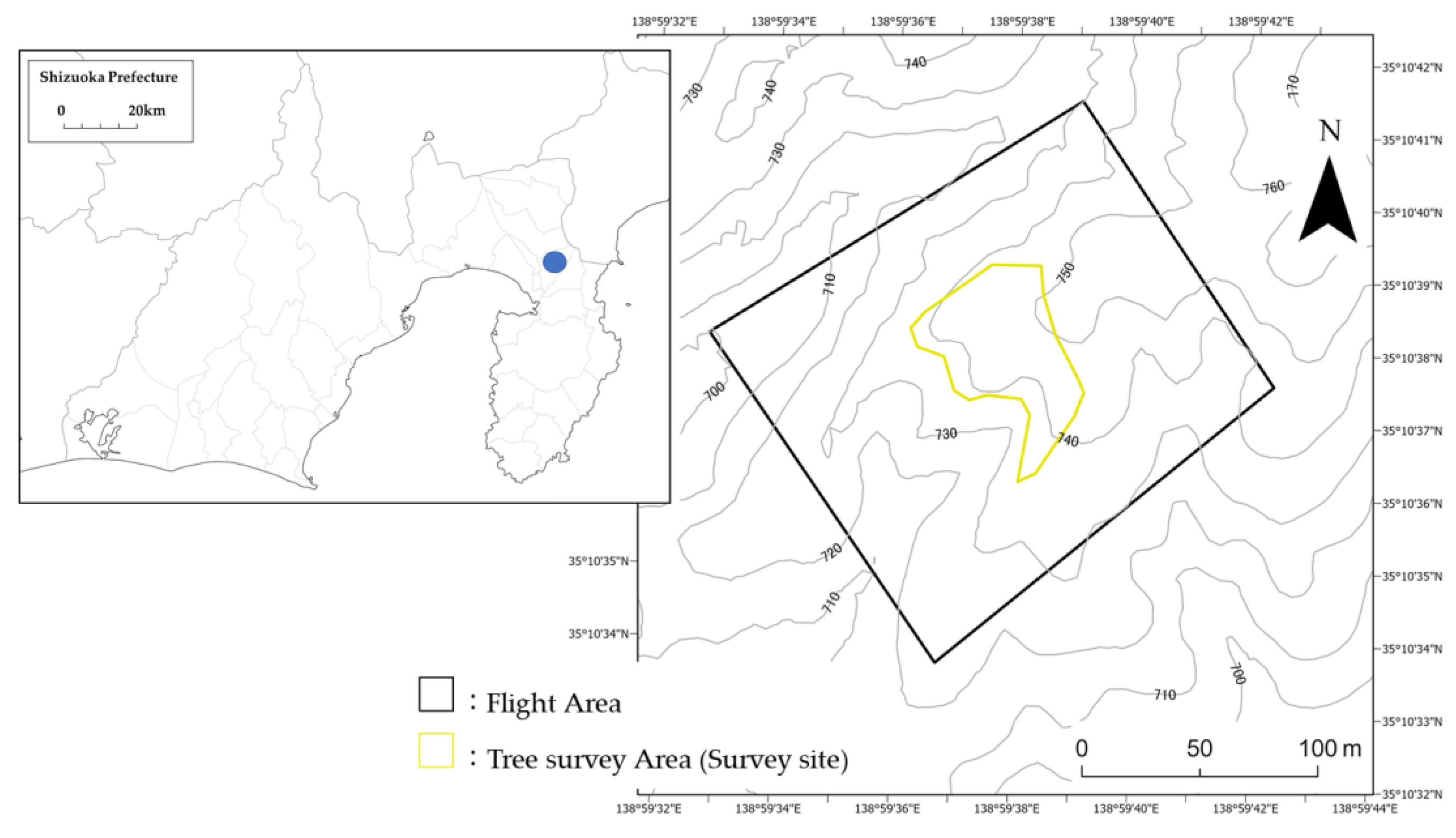
This study was conducted in the following sequence: (1) aerial image capture using UAVs, (2) SfM processing of aerial images and estimation of tree crown area and tree height, and (3) statistical analysis of the estimated values. (1) Aerial image capture using UAVs was performed as summarized in

Table 1. Overview of conditions pattern (date of capture, flight conditions, GCP number).

Pattern	Date of Capture	Flight Conditions Altitude (m)—Overlap (%)—Side Overlap (%)	GCP Numbers
A	January 2024	H100—OL90—SL90	4: Nos. 1, 2, 3′, 4
B	January 2024	H100—OL90—SL90	5: Nos. 1, 2, 3′, 4, 5
C	September 2023	H100—OL90—SL90	4: Nos. 1, 2, 3, 4
D	January 2024	H120—OL90—SL90	4: Nos. 1, 2, 3′, 4
E	January 2024	H120—OL90—SL90	5: Nos. 1, 2, 3′, 4, 5
F	July 2023	H120—OL90—SL90	4: Nos. 1, 2, 3, 4

. The analysis methods and parameters for each step are detailed below. Patterns A, B, and C are under the same flight conditions. However, compared to pattern A, pattern B has an increased number of GCPs, and when comparing patterns A and B to C, the environmental conditions around the GCPs differ. Also, patterns D, E, and F are under the same flight conditions. However, compared to pattern D, pattern E has an increased number of GCPs, and when comparing patterns D and E to F, the environmental conditions around the GCPs differ.

2.1. Survey Site

This study was conducted within a 0.32 ha area in Mishima City, Shizuoka Prefecture, Japan (Figure 1). The dominant tree species in the study site is Chamaecyparis obtusa, with some Cryptomeria japonica also present.

UAV photography was carried out in July and September 2023, as well as in January 2024 (Table 1). This study investigated the impact of the surrounding environment on GCP placement by the two survey patterns during different periods: one in July and September 2023, and another in January 2024. In July and September 2023, the survey area was surrounded by unused strip roads on two sides. When viewed from above, only this area and a small gap appeared open (Figure 2b). In the January 2024 survey, in addition to the strip roads observed in July and September 2023, new strip roads were constructed. As a result, the survey site became surrounded by strip roads on all four sides (Figure 2a). The survey was conducted at different times, so lighting may have influenced the results.

These changes in the survey area also led to differences in the surrounding environment of the GCP installation sites. GCPs No. 1 and No. 2 were installed in the same locations in both survey periods, with no observable changes in their surrounding environment. In the July and September 2023 survey, GCP No. 3 was placed on an existing strip road, where it was partially obscured by trees. However, by January 2024, the construction of a new strip road made the GCP more clearly visible from above (GCP No. 3 in January 2024 is referred to as GCP No. 3′). GCP No. 4 was initially installed in a forest gap during the 2023 survey. By January 2024, a newly constructed strip road was built nearby, eliminating canopy obstructions and making the GCP clearly recognizable from above. Additionally, with the construction of the strip road, more locations exhibited only slight numerical differences from the GCP. In contrast, during the July and September 2023 survey, the GCP was placed in a gap, leading to more significant variations in surrounding values. GCP No. 5 served as an added GCP in the January 2024 survey and was installed on the newly constructed strip road in a location that was easily recognizable from above. To summarize these differences, GCPs were installed around the survey area in both survey periods. In the 2023 survey, GCP panels were placed on existing strip roads and within forest gaps. In contrast, in the 2024 survey, the newly constructed strip roads made the GCPs more easily recognizable from above. Furthermore, the DSM values around the GCPs obtained from UAV-SfM showed only a slight difference when compared to the DTM values around the GCPs (DSM values = DTM values), resulting in continuous data. The coordinates of the GCPs were measured using GNSS devices (eTrex20 for GARMIN), and the elevation (Z value) was determined based on latitude and longitude information, referencing numerical data from the Geospatial Information Authority (GSI) map [61]. Moreover, each GCP was measured using four GNSS devices, and the average value was adopted as the coordinate for the GCP. However, the accuracy may have been influenced by the forest area.

The survey area (individual tree survey site) was established within the UAV flight zone, covering approximately 0.32 ha and including 151 target trees. The tree survey parameters included tree height and tree crown area. The tree height was measured five times using a VertexIII (Haglof) device, and the average value was taken as the tree’s height measurement. The tree crown area was measured using a 2 m pole. For each target tree, the distance from the trunk to the edge of the canopy was recorded in four directions: north, south, east, and west. These measurements were then used to calculate the canopy projection area based on a previously established method [62]. The average tree height of all target trees based on the measured values was 15.86 m (the minimum value for all target trees within the survey site was 12.16 m; the maximum value for all target trees within the survey site was 22.03 m; the average value of the standard deviation when measured five times for each target tree was 0.37 m). The estimated values derived from UAV-SfM for these 151 trees were compared against the measured values, which were considered the true reference data.

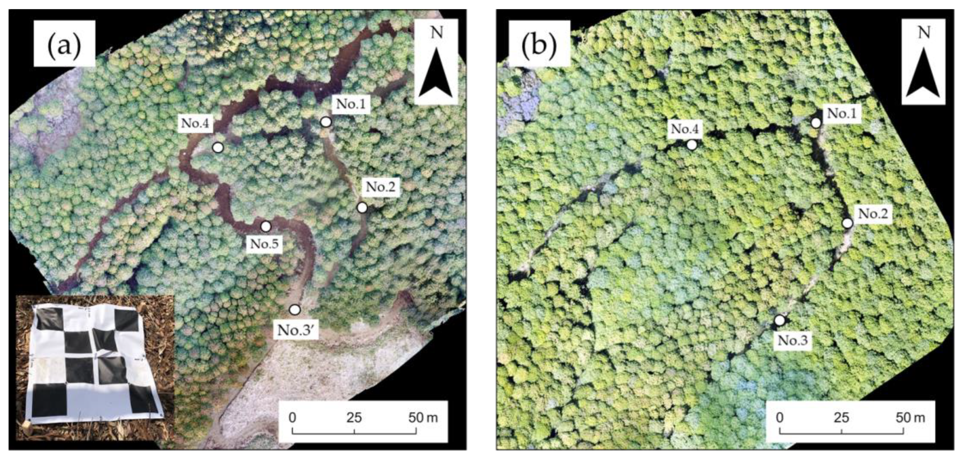
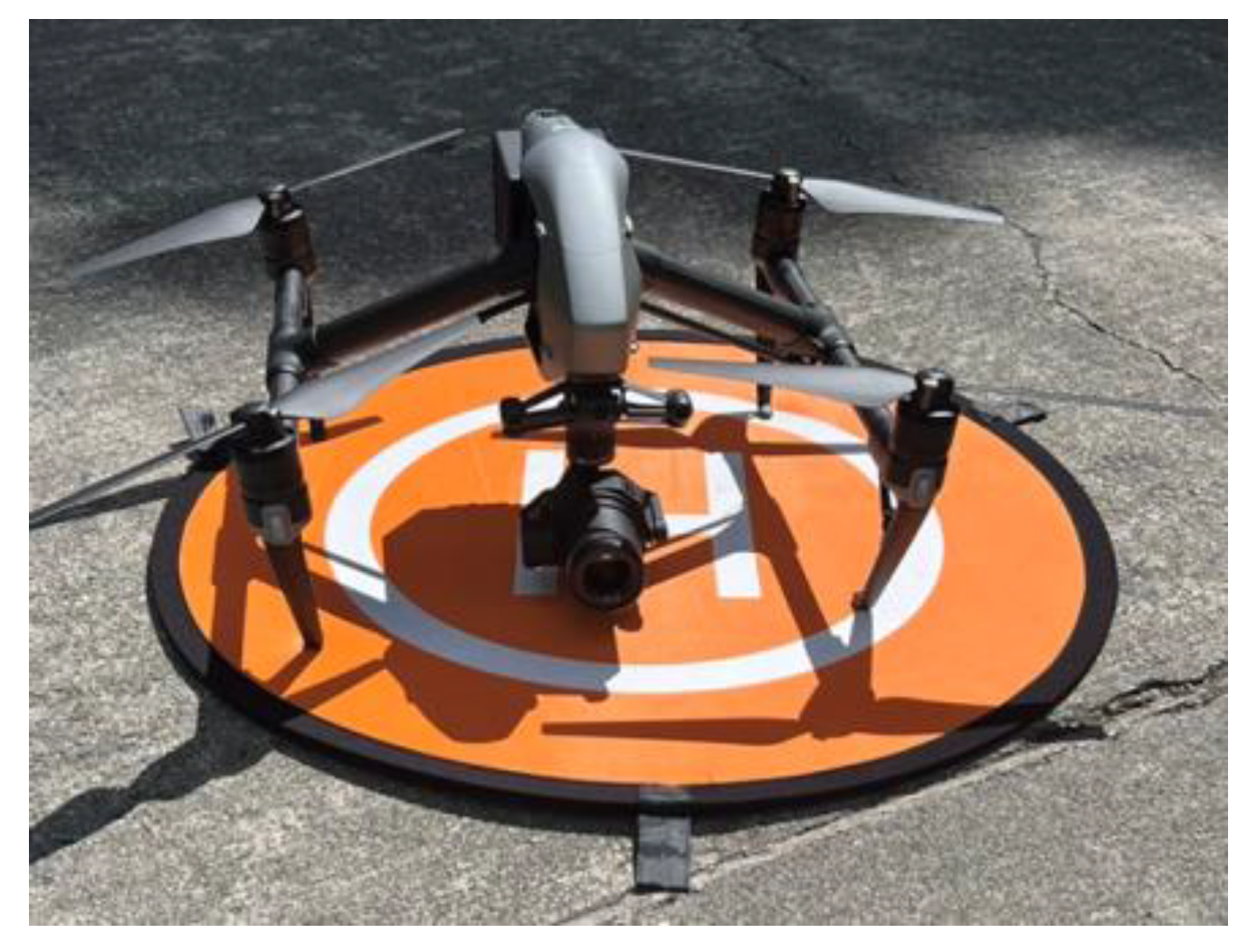
2.2. Aerial Image Capture Using an UAV

The UAV used for aerial imaging was the Inspire 2 from DJI, equipped with a Zenmuse X7 camera from DJI (Figure 3). The Inspire 2 weighs 3.4 kg (including two batteries but excluding the gimbal and camera), has dimensions of 605 mm (excluding propellers), a maximum flight time of approximately 23 min, and a maximum flight speed of 26 m/s [63].

Aerial imaging was conducted under sunny weather conditions, with wind speeds ranging from 0 to 5 m/s, between 10:00 and 13:00. The flight area covered approximately 1.4 ha, with an average slope of 20.6°. The UAV flight conditions are illustrated in Table 1. In July 2023 and January 2024, the flight altitude was 120 m, with both overlap and side overlap set to 90%. In September 2023, the flight altitude was 100 m, with both overlap and side overlap set to 90%. Additionally, in September 2023 and January 2024, the flight altitude was 100 m, with both overlap and side overlap set to 90%.

According to the Pix4D SfM software manual, it is recommended to increase both overlap and side overlap to at least 85% and to fly at a higher altitude for forested areas [51]. In addition, since the side overlap significantly affects the quality of the orthomosaic, it is necessary to set it to a high value [64]. To ensure optimal image processing, this study set the overlap and side overlap values higher than the recommended thresholds. For all flight conditions, the flight speed was set to 15.0 m/s. However, due to the high overlap rate, short capture intervals, and the imaging method being set to hovering mode, the UAV did not actually reach this speed. The hovering mode was specifically chosen to minimize noise in the captured images. These flight parameters were configured using the DJI GS PRO application (version 2.0.18) from DJI. Additionally, aerial photography was conducted using automatic flight. However, takeoff and landing were manually controlled by the operator to mitigate the risk of collisions with trees and potential crashes.

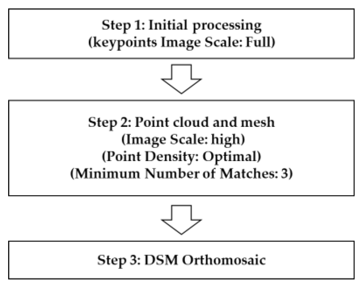
2.3. SfM Processing of Aerial Images and Estimation Method for Forest Resources

The SfM processing of aerial images using Pix4D (version 4.9.0) followed the procedure illustrated in Figure 4. The parameters for each step were configured to ensure simplicity, making the process accessible to general users—in this case, on-site forestry workers without specialized expertise. To achieve this, the parameters were set according to the Pix4D user manual [51], adhering to the recommended values. Referring to the manual was expected to enhance the universality and reproducibility of the results.

The estimation of forest information using UAV data was conducted based on 3D point cloud data and orthomosaic images generated in Step 3 of Figure 4, along with a 5 m DTM obtained from the Geospatial Information Authority of Japan’s airborne LiDAR surveying with a height accuracy (root mean square error) of 0.3 m [20].

ArcGIS Pro (version 3.2.1) was used for the analysis. Tree height estimation followed the following steps: (1) the DCHM was calculated by subtracting the 5 m DTM from the DSM derived from the 3D point cloud data, (2) tree top points were extracted from the DCHM data, and (3) the DCHM value at each extracted tree top location was used as the estimated tree height. This method was based on the UAV manual of the Forestry Agency [16]. For tree crown area estimation, multiple tree top points were occasionally extracted for a single target tree. When the target tree could not be accurately identified, orthomosaic and tree top data were used as references. The measurement function in ArcGIS Pro was then applied for manual measurements.

2.4. Accuracy of the Estimated Values

To compare the estimated values (derived from UAV-SfM) with the true values (obtained from tree survey measurements), the error (RMSE) and the relative root mean square error (rRMSE) were calculated using the following formulas:

$$\mathrm{R}\mathrm{M}\mathrm{S}\mathrm{E}=\sqrt{{\displaystyle \frac{{\sum }_{i=1}^n{\left(y_i-{\acute{y}}_i\right)}^2}{n}}}$$

(1)

$$\mathrm{r}\mathrm{R}\mathrm{M}\mathrm{S}\mathrm{E}\left[\%\right]={\displaystyle \frac{RMSE}{\overline{y}}}\times 100$$

(2)

where n is the total number of samples, $y_i$ represents the predicted values, ${\acute{y}}_i$ denotes the observed values, and $\overline{y}$ is the mean of the observed values.

Additionally, a one-way analysis of variance (ANOVA) was conducted to compare the estimated and true values, as well as differences between flight conditions. Statistical significance was determined at p < 0.05, and post hoc analysis was performed using Bonferroni multiple comparisons with a significance level of p < 0.05.

3. Results

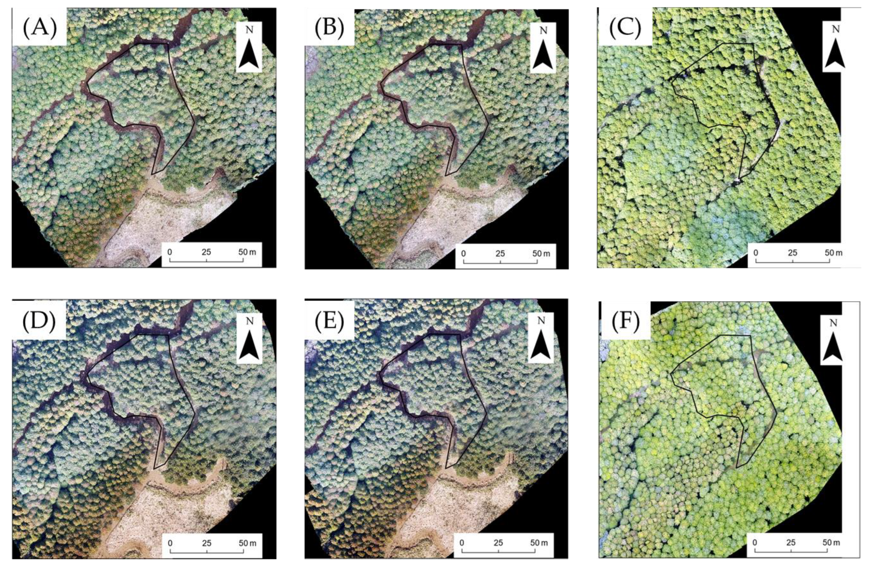
3.1. SfM Processing of Aerial Images

The DSM and orthomosaic images are shown in Figure 5 and Figure 6.

The processing results of the aerial images captured by the UAV are shown in

Table 2. The detailed processing results of the aerial images by p.

FCP	NC/NT	MRE (pix)	GSD (cm)	NDP (Points)	AD (per m2)
A	226/226	0.176	1.22	32,136,053	1300
B	226/226	0.176	1.17	32,554,781	1513
C	195/195	0.249	1.33	23,634,621	695
D	158/158	0.185	1.49	22,542,910	639
E	158/158	0.21	1.39	22,679,108	813
F	140/140	0.169	1.48	18,220,310	526

Note: FCP = Flight condition pattern; NC = Number of camera calibrated aerial images; NT = Number of aerial images taken; MRE = Mean reprojection error; GSD = Ground sampling distance; NDP = Number of densified points; AD = Average density.

. Camera calibration was successfully completed for all images across all flight conditions, relative to the number of shots taken. Under similar flight conditions, the number of images varied depending on the time of capture. This variation resulted from the need to fully model the surrounding strip roads, leading to changes in the range of captured areas. Consequently, direct comparisons were challenging. However, conditions with fewer images (pattern C and D) exhibited lower high-density point cloud generation and a reduced average point cloud density. At the same flight altitude, ground resolution remained largely unaffected. However, patterns B and C where the surrounding area was open and additional GCPs were used produced more detailed ground sampling distances (GSDs), with values of 1.17 and 1.39 cm, respectively, compared to the other conditions. The mean reprojection error at a flight altitude of 100 m was the highest in pattern C, where the GCP area was closed, with a value of 0.249 pixels. At the same altitude of 120 m, pattern E had the highest reprojection error of 0.21 pixels. Conversely, at a flight altitude of 120 m, pattern F exhibited the lowest mean reprojection error. Overall, differences in the surrounding environment of GCPs and the number of GCPs had a minimal impact, indicating that these factors had little effect on the results.

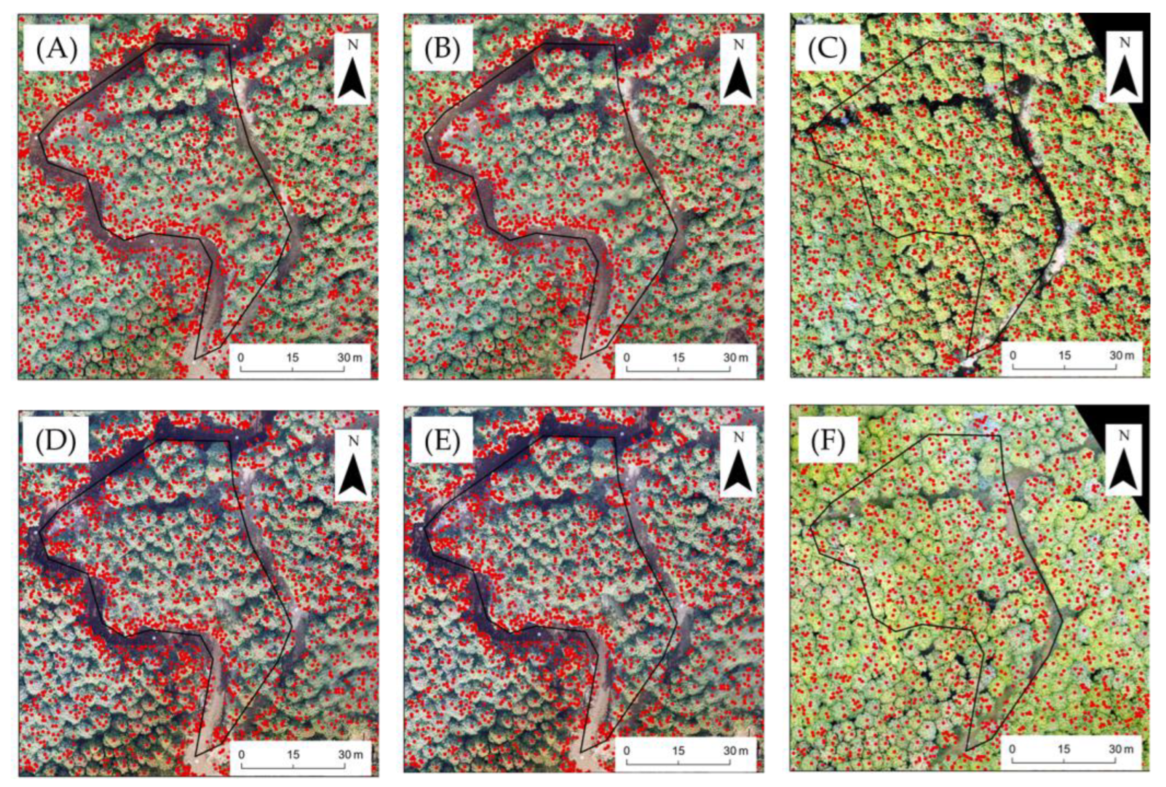
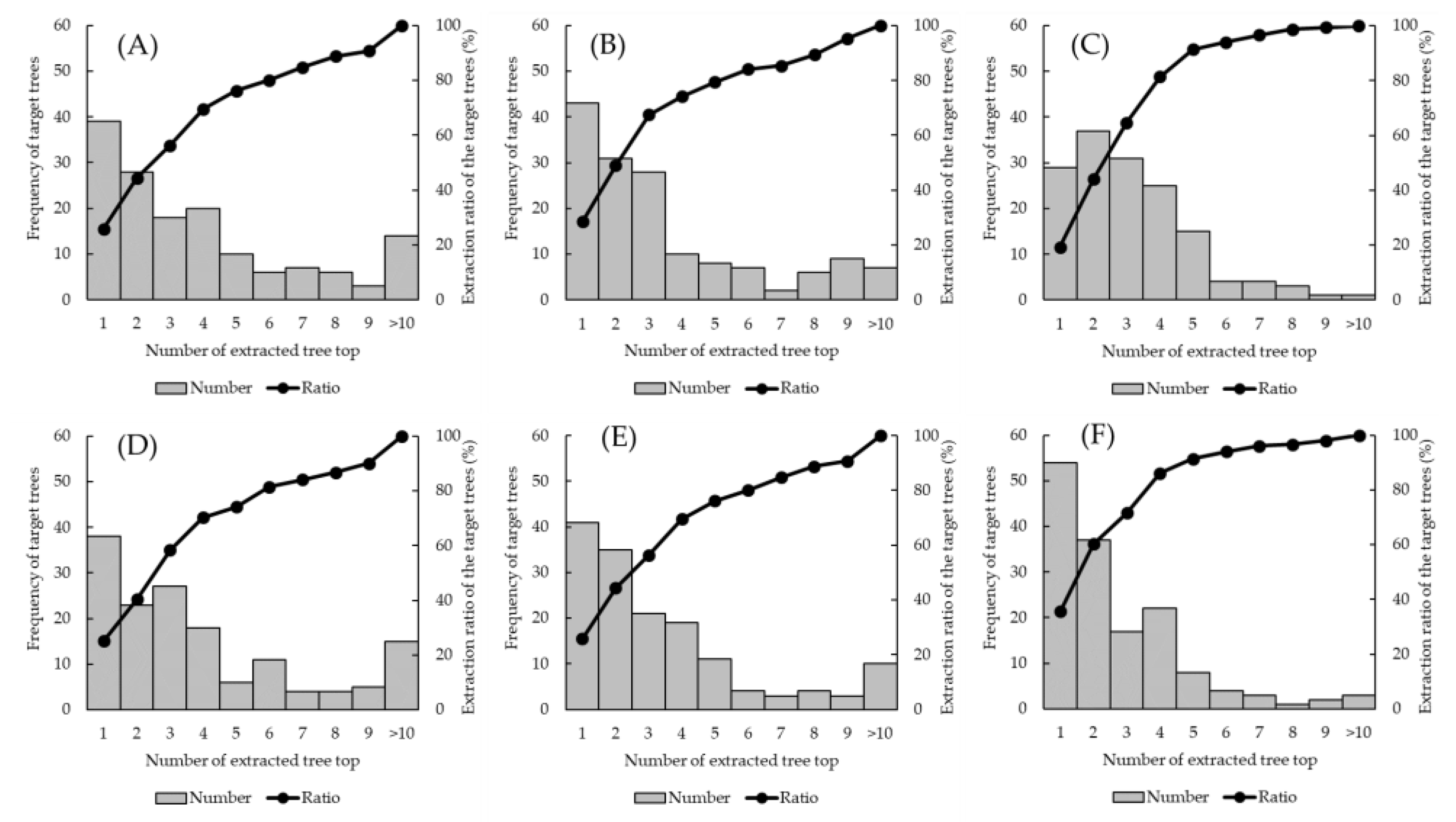
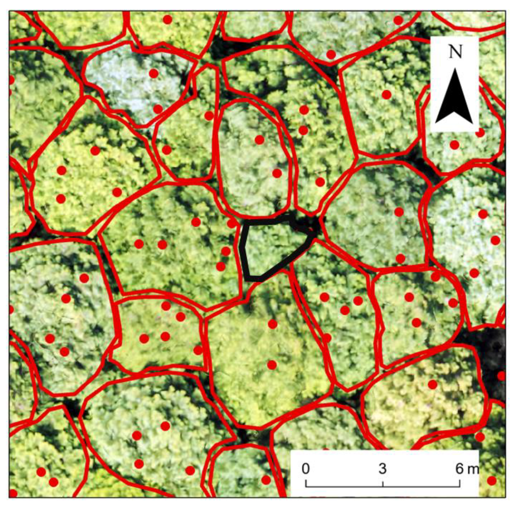
3.2. Extraction Target Trees

Figure 7 shows the results of the tree top extraction.

In patterns A, B, and D–F, all target trees within the survey area were successfully extracted. However, in pattern C, one target tree was not extracted. Figure 8 presents histograms of the tree top extraction results for each pattern, indicating that when one or more tree tops were extracted for a single target tree, noise (where multiple tree tops were marked for the same tree) was likely present. When assessing the number of target trees marked with only one tree top (indicating no noise), pattern F had the highest count, with 51 trees (35.8% of the total target trees), while pattern C had the lowest, with 29 trees (29.3% of the total target trees). The other patterns showed a range of approximately 40 trees (25.2% to 28.5% of the total target trees), with no significant differences. Additionally, in all patterns, the number of target trees marked with five or fewer tree tops was over 70%. However, in patterns C and F, this percentage increased to 91%, suggesting that closed surroundings resulted in fewer instances of noise. Trees marked with five or more tree tops were more frequently located at the forest edge, where neighboring trees were not visible.

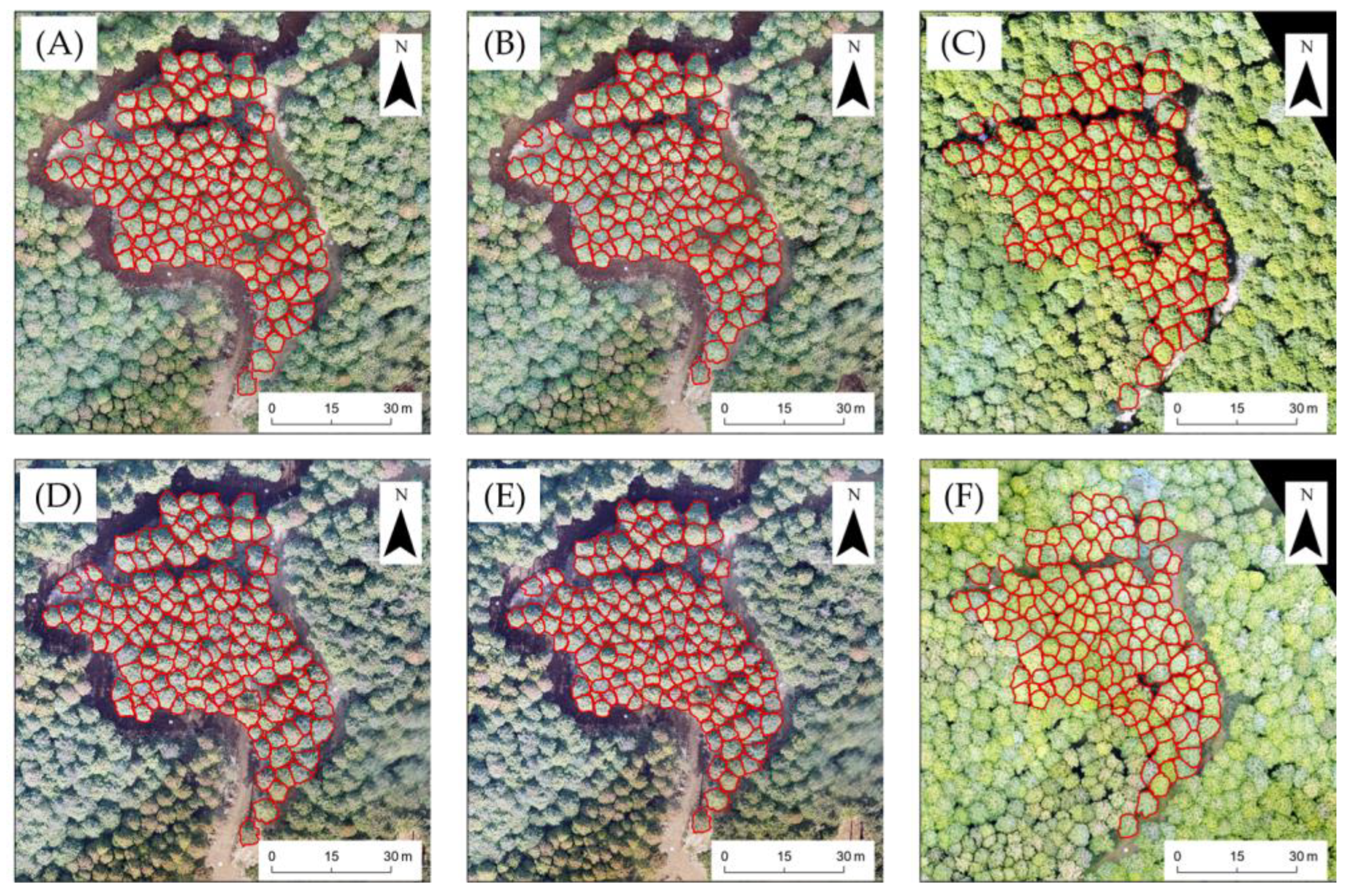
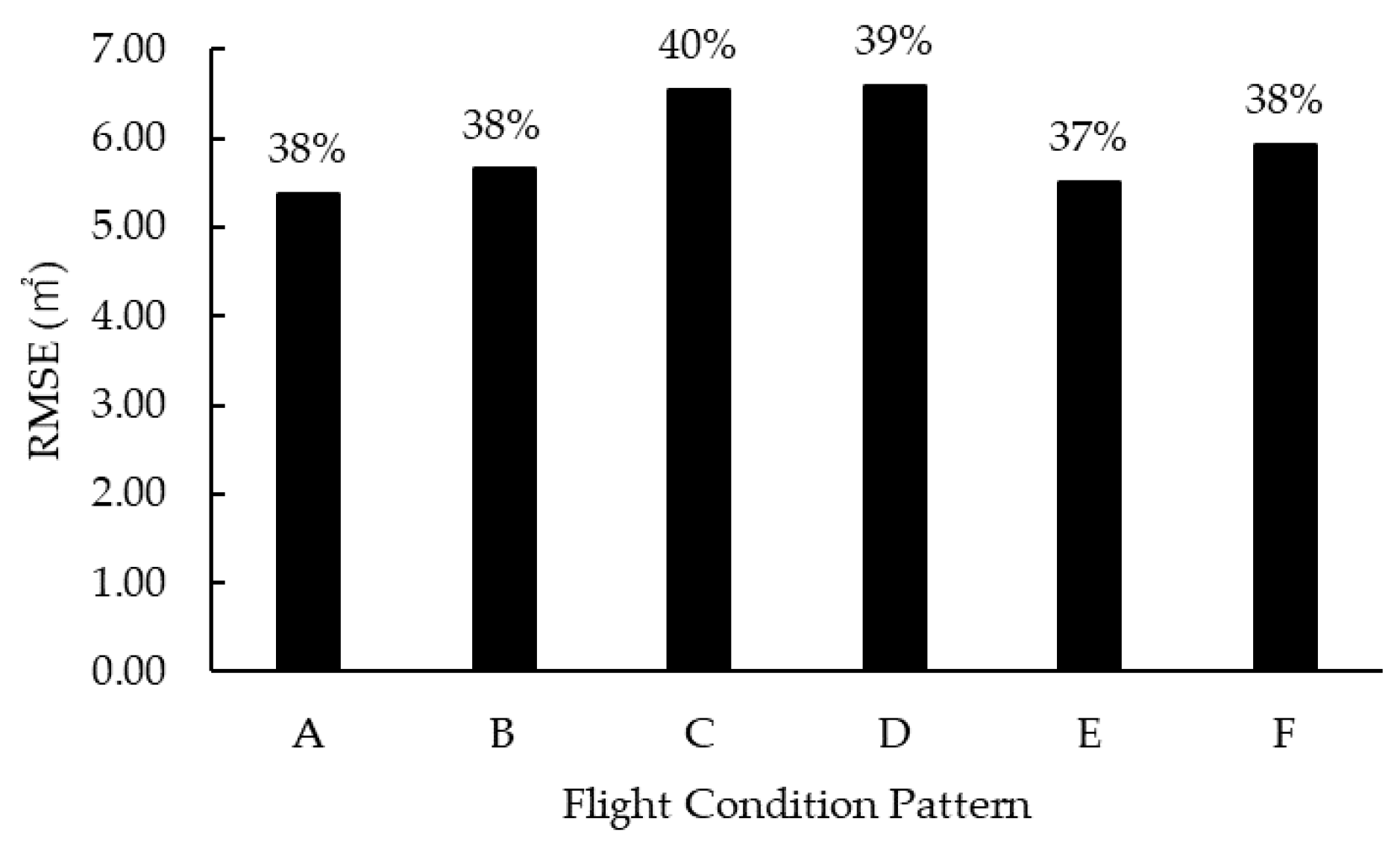
3.3. Estimated Crown Area

Figure 9 shows the manually marked tree crown area.

Figure 10 presents the scatter plot and regression line comparing the field-measured tree crown area with UAV-SfM estimated values for each pattern. No significant trends were observed between the measured and estimated values in the scatter plot. However, across all flight conditions, lower measured values tended to be overestimated compared to field measurements. In all patterns, the coefficient of determination (R²) ranged from approximately 0.21 to 0.24, indicating a weak correlation.

Figure 11 shows the RMSE between the field-measured tree crown area and the UAV-SfM estimated values. The highest accuracy was observed in pattern A, with an RMSE of 5.38 m² (rRMSE = 38.09%). In the other patterns, RMSE values ranged from approximately 5 to 6.5 m², with rRMSE values between 36% and 39%. These results indicate that increasing the number of GCPs or modifying the surrounding environment of GCPs did not improve the accuracy of tree crown area estimation. Additionally, field measurements revealed that trees located at the forest edge, where they did not come into contact with neighboring trees, tended to have higher estimated tree crown areas compared to other trees. Conversely, in more densely populated areas, measured values tended to underestimate the actual tree crown area.

ANOVA with paired data was performed to compare the estimated and actual tree crown area values for each pattern. The results (p < 0.01) indicated a statistically significant difference (p < 0.05). Consequently, a Bonferroni post hoc test was conducted, and the results of the multiple comparisons are shown in

Table 3. p-values for the multiple comparisons of the tree crown area for each pattern.

	MV	A	B	C	D	E	F
MV	×	0.146	<0.001 **	<0.001 **	<0.001 **	<0.001 **	<0.001 **
A	—	×	0.030 *	<0.001 **	<0.001 **	0.124	<0.001 **
B	—	—	×	<0.001 **	<0.001 **	1	0.132
C	—	—	—	×	1	<0.001 **	0.131
D	—	—	—	—	×	<0.001 **	0.004 **
E	—	—	—	—	—	×	0.032 *
F	—	—	—	—	—	—	×

Note: The numbers in the table represent the p-values for each combination; MV = Measured values; A to F = test patterns; * = p < 0.05; ** = p < 0.01.

. When compared to field measurements, no statistically significant difference was observed between the actual values and only pattern A. There was no statistically significant difference observed between the estimated values at the same flight altitude. These findings suggest that modifying the surrounding environment or increasing the number of GCPs had no significant effect on tree crown area estimation.

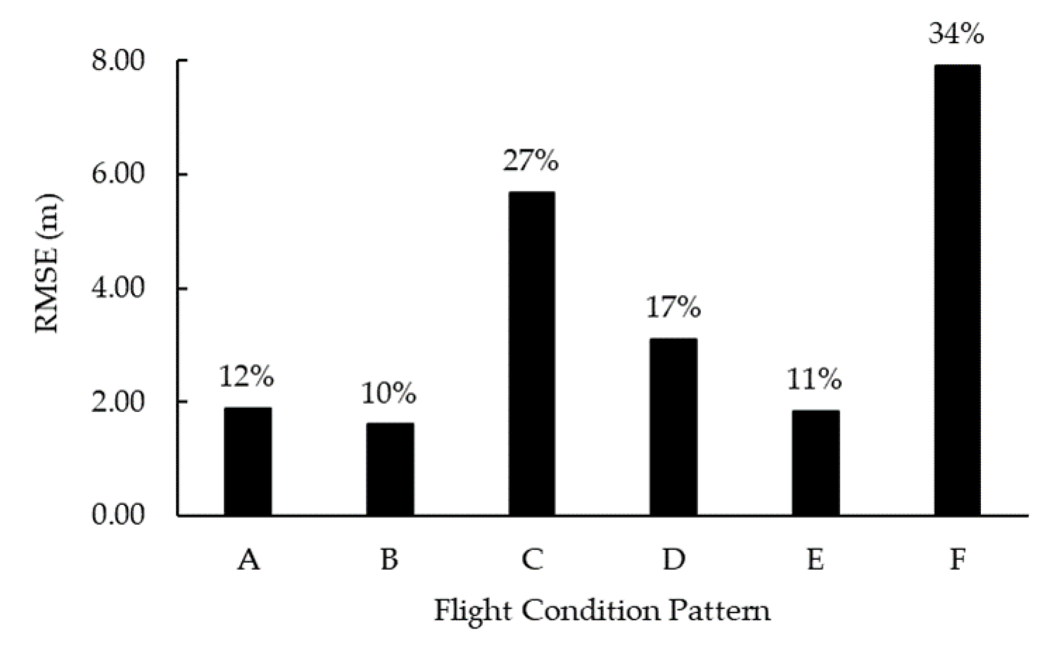
3.4. Estimated Tree Height

Figure 12 shows a scatter plot and regression line comparing the field-measured tree height with UAV-SfM estimated values. For patterns A, B, D, and E, the R² values ranged from 0.15 to 0.29, indicating no correlation or a weak correlation. However, when comparing patterns A and B or patterns D and E, an increasing number of GCPs corresponded to higher R² values. Additionally, for patterns C and F, the R² values were 0.76 and 0.69, respectively, indicating a strong correlation. However, both conditions exhibited a tendency to overestimate tree height.

Figure 13 shows the RMSE between field-measured tree height and UAV-SfM estimated values. The highest accuracy was obtained under pattern B, with an RMSE of 1.60 m (rRMSE = 10.06%). In contrast, the lowest accuracy was observed under pattern F, with an RMSE of 7.92 m (rRMSE = 33.61%). When comparing similar flight conditions, those in which GCPs were in open surroundings and for which data were collected in January 2024 (those of pattern A, B, D, and E ranged between 1.60 to 3.09 m) exhibited higher-accuracy patterns C and D (RMSE = 5.69 to 7.92 m). Additionally, increasing the number of GCPs improved the estimation accuracy.

ANOVA with paired data was conducted to compare the estimated and actual tree height values under each pattern. The results indicated a statistically significant difference (p < 0.01), confirming that the estimated values differed from the actual values (p < 0.05). Consequently, a Bonferroni post hoc test was performed, and the results of the multiple comparisons are presented in

Table 4. p-values for the multiple comparisons of tree height for each pattern.

	MV	A	B	C	D	E	F
MV	×	0.677	1	<0.001 **	<0.001 **	0.196	<0.001 **
A	—	×	0.321	<0.001 **	<0.001 **	<0.001 **	<0.001 **
B	—	—	×	<0.001 **	<0.001 **	0.432	<0.001 **
C	—	—	—	×	<0.001 **	<0.001 **	<0.001 **
D	—	—	—	—	×	<0.001 **	<0.001 **
E	—	—	—	—	—	×	<0.001 **
F	—	—	—	—	—	—	×

Note: The numbers in the table represent the p-values for each combination; MV = measured values; A to F = test patterns; ** = p < 0.01.

. When compared to the actual values, no statistically significant differences were observed for pattern A (p = 0.677) and pattern B (p = 1.00). However, for patterns D and E, a statistically significant difference was found in pattern D (p < 0.001), while no significant difference was observed in pattern E (p = 0.196). Additionally, a statistically significant difference was found between patterns C and F (p < 0.001). For comparisons at the same altitude, no significant difference was observed between patterns A and B, but significant differences were identified between patterns A and C, as well as between patterns B and C. Furthermore, significant differences were found among all combinations of patterns D, E, and F.

These results suggest that when the GCP surroundings were open, the difference between the estimated and actual values decreased, leading to more accurate estimations. Moreover, increasing the number of GCPs further improved estimation accuracy.

4. Discussion

The results of this study indicate that while variations in the surrounding environment of GCPs and an increase in their number have only a minor impact on SfM processing results, tree top extraction, and tree crown area estimation, they significantly improve tree height estimation accuracy. I believe that this result is novel and has not been reported in previous research.

Regarding the number of extracted trees, instances of prevalent noise were observed. The method for noise removal follows the guidelines outlined in the Forestry Agency’s manual [16], where adjusting noise removal parameters alters tree extraction results. In this study, noise removal was conducted based on the manual’s recommended values. However, automatic noise removal was not applied, and parameters were manually adjusted. Notably, modifying noise removal parameters allows for easy noise reduction. Noise was particularly prevalent at the forest edge, likely due to misidentification of tree tops caused by the expanded canopy spread in these areas.

Noise was particularly prevalent at the forest edge, and the expanded tree crown area may have led to the misidentification of tree tops. Previous studies have reported that areas with significant overlap of multiple tree crowns or narrow tree crown spacing make it difficult to detect trees [65]. Therefore, the forest edge can be considered an area with minimal overlap of tree crowns or wider crown spacing, which likely led to more vigorous plant growth, making the trees easier to detect. However, vertical accuracy is generally lower than horizontal accuracy [44,45,46,47]. Therefore, since horizontal errors are small [44,45,46,47], the relative error in the tree crown structure is likely also small. Consequently, the impact of differences in the surrounding environment of GCPs and the number of GCPs is considered to be minimal. The results of these previous studies also contribute to tree crown area estimation. Moreover, the factors contributing to the target trees that could not be extracted include, according to previous studies, areas with significant overlap of multiple tree crowns and narrow tree crown spacing, which make it difficult to detect trees [65]. The tree crown area of non-extracted target trees was the smallest at 4.97 m² (average value of the estimates from the six patterns), which indicates significant overlap of multiple tree crowns (the target tree that could not be extracted and the surrounding tree conditions are shown in Figure 14). Therefore, similar to the factors identified in previous studies, some tree crowns were not detected due to overlap with other tree crowns.

The surrounding environment and the number of GCPs did not significantly affect crown area estimation but had a measurable impact on tree height estimation. Conversely, in tree crown area estimation, factors such as the presence of neighboring trees and potential suppression from surrounding vegetation likely influenced the results. Changes in the surrounding environment, particularly those caused by strip road construction, may have led to an overestimation of target tree dimensions, contributing to estimation errors. Additionally, compared to tree height, the estimation results for the tree crown area showed lower accuracy (higher RMSE values), which aligns with the results of a previous study [66]. Specifically, direct visual measurement is possible in a field setting. However, from an aerial perspective, overlapping tree crown areas make it difficult to accurately grasp the forest structure, which is likely the cause of this discrepancy. In this study, the difference in the number of GCPs considered was only one (i.e., there were either four or five GCPs). However, in forest areas, the locations in which GCPs can be placed are limited, and measuring GCPs involves time and costs. Thus, reducing the GCP number likely improves work and cost efficiency.

In tree height estimation, it is necessary to correct the X and Y coordinates when calculating differences from a DTM, and correcting the Z value is even more critical [44,45,46,47]. Increasing the number of known coordinate points (i.e., GCPs) improved estimation accuracy by enhancing positional correction. The RMSE of tree height estimation was more accurate (smaller RMSE values) when the environment surrounding GCPs was open. Additionally, increasing the number of GCPs allowed for more accurate estimations. In particular, the RMSE values for patterns A, B, and E were comparable to those reported in previous studies [66,67]. However, the RMSE of the tree height estimations by Krause et al. [68] was below 0.5 m, indicating higher accuracy that in the current study. Krause et al. [68] performed GCP coordinate measurements using total stations, which requires additional time and costs. Additionally, the quality of the GCP locations depends on the survey grade for collecting the GCPs, as well as the accuracy of the GNSS and total station equipment [34,40,69]. In this study, a simple handheld GNSS was used. Therefore, use of more precise GNSS equipment is necessary to achieve the same level of accuracy as in the previous study [68]. Additionally, in the study by Volga et al. [70], eight GCPs were used for tree height measurement, and the RMSE for the related Pix4D results was 0.57. Since the authors utilized more GCPs than this study, an increase in the number of GCPs likely improves the accuracy of tree height estimations. However, measuring GCPs requires additional time and cost [32,68]. Moreover, halving the number of GCPs could significantly reduce the labor required in the field [30]. Additionally, after proper reconstruction of the terrain using photogrammetry, the horizontal accuracy is high, commonly less than 10 cm, and the vertical accuracy is less than 20 cm, allowing for highly precise measurements [69]. An increase in distortion due to elevation differences between the UAVs and the ground sometimes make it difficult to identify the GCPs from UAV aerial images [71]. In forested areas, it is difficult to read the terrain, and high-altitude flights are required to avoid collisions between the UAV and trees. These factors may challenge the use of UAVs in forested areas. The number of GCPs (i.e., increasing the number), their placement (e.g., placing them around the survey area or in all corners), and how their location information is obtained, as discussed in previous studies, are important factors that determine the feasibility of the UAV approach. Additionally, the results of this study indicate that an open environment around the GCPs, such as along strip roads, led to an improvement in tree height estimation accuracy. Thus, the environment surrounding GCPs is likely an important factor in UAV-SfM-based forest resource assessment.

Several external factors may have influenced the results of the SfM analysis, individual tree extraction, and tree height and crown area estimations. These factors include meteorological conditions such as light and wind. In this study, imagery was captured in July and September, before environmental changes, and in January, after these changes. Efforts were made to minimize the influence of meteorological conditions by maintaining consistent flight times and wind speeds. However, despite controlling for time of day, seasonal variations in the Sun’s angle may have altered shadow directions and light intensity. Moreover, plant activity levels can fluctuate with seasonal changes. The effects of seasons and light on the complexity of tree shadows should not be ignored, and this may have introduced a certain degree of error [72]. Surveys should be conducted under relatively cloudy conditions with minimal direct sunlight [73]. Strong light can cause shadows on adjacent trees, leading to misidentification of gaps [73]. It has also been reported that the state of plant activity varies with the seasons, which can affect tree classification [74]. Moreover, calibration of non-metric cameras is sensitive to poor lighting conditions [75]. By improving the quality and density of the point cloud representing the tree crown through parameter selection of lens distortion models, the accuracy of tree trunk area estimations can be enhanced [76]. All of these factors may have influenced the result of this study. Future research should carefully assess and account for these variables to ensure more accurate and reliable estimations.

5. Conclusions

This study examined the impact of the number of GCPs and variations in their surrounding environment when estimating forest resource quantities using UAV-based SfM. The following conclusions can be drawn:

• The effect of GCPs on SfM image processing and tree count or tree crown area estimations was minimal.
• Increasing the number of GCPs and ensuring an open surrounding environment improved the accuracy of tree height estimation.

These results suggest that in forest resource surveys using UAV-based SfM, particularly for tree height estimation, not only the number and placement of GCPs but also the surrounding environment play a crucial role in improving estimation accuracy. These are important findings that have been clarified through this study. It is difficult to find large gaps in forested areas; however, in the case of long-term monitoring, it may be effective to actively place GCPs in cleared areas where activities such as strip road construction or thinning have taken place for forest management. The findings of this study provide valuable insights for users applying UAV-SfM in forest areas. The author previously examined the impact of UAV flight conditions and SfM software [13,14,15]. In the future, it is considered necessary to take into account the impact of variations in light conditions due to seasonal differences. Continued research and investigation in this field remain essential. In UAV-SfM-based forest resource surveys, analyzing factors that influence estimation accuracy is critical for practical applications in forested environments.

References

1. Torresan, C.; Berton, A.; Carotenuto, F.; Di Gennaro, S.F.; Gioli, B.; Matese, A.; Miglietta, F.; Vagnoli, C.; Zaldei, A.; Wallace, L. Forestry applications of UAVs in Europe: A review. Int. J. Remote Sens. 2017, 38, 2427–2447. [Google Scholar] [CrossRef]
2. Guimarães, N.; Pádua, L.; Marques, P.; Silva, N.; Peres, E.; Sousa, J.J. Forestry remote sensing from unmanned aerial vehicles: A review focusing on the data, processing and potentialities. Remote Sens. 2020, 12, 1046. [Google Scholar] [CrossRef]
3. Tong, H.; Yuan, J.; Zhang, J.; Wang, H.; Li, T. Real-time wildfire monitoring using low-altitude remote sensing imagery. Remote Sens. 2024, 16, 2827. [Google Scholar] [CrossRef]
4. Kanaskie, C.R.; Routhier, M.R.; Fraser, B.T.; Congalton, R.G.; Ayres, M.P.; Garnas, J.R. Early detection of southern pine beetle attack by UAV-collected multispectral imagery. Remote Sens. 2024, 16, 2608. [Google Scholar] [CrossRef]
5. Taki, S.; Nakazawa, M.; Akamatsu, H. Interpretation of forestry work road networks by using small fixed-wing UAV. J. Jpn. For. Eng. Soc. 2020, 35, 147–151. [Google Scholar] [CrossRef]
6. Taki, S.; Takata, K.; Inakawa, K. Interpretation of forestry work road networks by a small, unmanned multicopter. Jpn. J. For. Plann. 2016, 50, 41–49. [Google Scholar] [CrossRef]
7. Li, T.; Lin, J.; Wu, W.; Jiang, R. Effects of illumination conditions on individual tree height extraction using UAV LiDAR: Pilot study of a planted coniferous stand. Forests 2024, 15, 758. [Google Scholar] [CrossRef]
8. Zhou, X.; Ma, K.; Sun, H.; Li, C.; Wang, Y. Estimation of forest stand volume in coniferous plantation from individual tree segmentation aspect using UAV-LiDAR. Remote Sens. 2024, 16, 2736. [Google Scholar] [CrossRef]
9. Taki, S.; Aoki, M.; Koujimaru, M.; Inada, J. Aerial photography for in-forest using an artificial intelligence-enabled drone, and the construction of an in-forest three-dimensional model. J. Jpn. For. Eng. Soc. 2021, 36, 151–160. [Google Scholar] [CrossRef]
10. Htun, N.M.; Owari, T.; Tsuyuki, S.; Hiroshima, T. Detecting canopy gaps in uneven-aged mixed forests through the combined use of unmanned aerial vehicle imagery and deep learning. Drones 2024, 8, 484. [Google Scholar] [CrossRef]
11. Huang, Y.; Ou, B.; Meng, K.; Yang, B.; Carpenter, J.; Jung, J.; Fei, S. Tree species classification from UAV canopy images with deep learning models. Remote Sens. 2024, 16, 3836. [Google Scholar] [CrossRef]
12. Silva, B.R.F.d.; Ucella-Filho, J.G.M.; Bispo, P.d.C.; Elera-Gonzales, D.G.; Silva, E.A.; Ferreira, R.L.C. Using drones for dendrometric estimations in forests: A bibliometric analysis. Forests 2024, 15, 1993. [Google Scholar] [CrossRef]
13. Kameyama, S.; Sugiura, K. Estimating tree height and volume using unmanned aerial vehicle photography and SfM technology, with verification of result accuracy. Drones 2020, 4, 19. [Google Scholar] [CrossRef]
14. Kameyama, S. Verification of measurement accuracy on forest information and work efficiency in UAV-SfM by double grid flight. Kanto J. For. Res. 2024, 75, 89–92. [Google Scholar]
15. Kameyama, S.; Sugiura, K. Effects of differences in structure from motion software on image processing of unmanned aerial vehicle photography and estimation of crown area and tree height in forest. Remote Sens. 2021, 13, 626. [Google Scholar] [CrossRef]
16. Forestry Agency. UAV Timber Cruise Manual. Available online: https://www.rinya.maff.go.jp/j/gyoumu/gijutu/attach/pdf/syuukaku_kourituka-2.pdf (accessed on 15 February 2025). (In Japanese).
17. Forestry Agency. UAV Photogrammetry Manual. Available online: https://www.rinya.maff.go.jp/j/sekou/gijutu/attach/pdf/ICT_seko-49.pdf (accessed on 15 February 2025). (In Japanese).
18. Akita Prefecture. Manual for Forest Resource Survey Using Photos Taken by Drones. Available online: https://www.pref.akita.lg.jp/pages/archive/80172 (accessed on 15 February 2025). (In Japanese).
19. Shizuoka Prefecture. Forest Resource Measurement Using Drones. Available online: https://www.pref.shizuoka.jp/_res/projects/default_project/_page_/001/054/615/670.pdf (accessed on 15 February 2025). (In Japanese).
20. Geospatial Information Authority of Japan. Fundamental Geospatial Data. Available online: https://fgd.gsi.go.jp/download/menu.php (accessed on 15 February 2025). (In Japanese).
21. Kalacska, M.; Lucanus, O.; Arroyo-Mora, J.P.; Laliberté, É.; Elmer, K.; Leblanc, G.; Groves, A. Accuracy of 3D landscape reconstruction without ground control points using different UAS platforms. Drones 2020, 4, 13. [Google Scholar] [CrossRef]
22. Seo, D.-M.; Woo, H.-J.; Hong, W.-H.; Seo, H.; Na, W.-J. Optimization of number of GCPs and placement strategy for UAV-based orthophoto production. Appl. Sci. 2024, 14, 3163. [Google Scholar] [CrossRef]
23. Zhang, K.; Okazawa, H.; Hayashi, K.; Hayashi, T.; Fiwa, L.; Maskey, S. Optimization of ground control point distribution for unmanned aerial vehicle photogrammetry for inaccessible fields. Sustainability 2022, 14, 9505. [Google Scholar] [CrossRef]
24. Sanz-Ablanedo, E.; Chandler, J.H.; Rodríguez-Pérez, J.R.; Ordóñez, C. Accuracy of unmanned aerial vehicle (UAV) and SfM photogrammetry survey as a function of the number and location of ground control points used. Remote Sens. 2018, 10, 1606. [Google Scholar] [CrossRef]
25. Atik, M.E.; Arkali, M. Comparative assessment of the effect of positioning techniques and ground control point distribution models on the accuracy of UAV-based photogrammetric production. Drones 2025, 9, 15. [Google Scholar] [CrossRef]
26. Yu, J.J.; Kim, D.W.; Lee, E.J.; Son, S.W. Determining the optimal number of ground control points for varying study sites through accuracy evaluation of unmanned aerial system-based 3D point clouds and digital surface models. Drones 2020, 4, 49. [Google Scholar] [CrossRef]
27. Lalak, M.; Wierzbicki, D.; Kędzierski, M. Methodology of processing single-strip blocks of imagery with reduction and optimization number of ground control points in UAV photogrammetry. Remote Sens. 2020, 12, 3336. [Google Scholar] [CrossRef]
28. Ferrer-González, E.; Agüera-Vega, F.; Carvajal-Ramírez, F.; Martínez-Carricondo, P. UAV photogrammetry accuracy assessment for corridor mapping based on the number and distribution of ground control points. Remote Sens. 2020, 12, 2447. [Google Scholar] [CrossRef]
29. Koshimizu, K.; Kawakami, G.; Ebina, M.; Ishimaru, S.; Urabe, A. Effective GCP layout on UAV-SfM survey for steep cliffs. Trans. Jpn. Geomorphol. Union 2020, 41, 1–13. [Google Scholar] [CrossRef]
30. James, M.R.; Robson, S.; d’Oleire-Oltmanns, S.; Niethammer, U. Optimising UAV topographic surveys processed with structure-from-motion: Ground control quality, quantity and bundle adjustment. Geomorphology 2017, 280, 51–66. [Google Scholar] [CrossRef]
31. Zhong, H.; Duan, Y.; Tao, P.; Zhang, Z. Influence of ground control point reliability and distribution on UAV photogrammetric 3D mapping accuracy. Geo-spatial Inf. Sci. 2025. ahead-of-print. [Google Scholar] [CrossRef]
32. Ulvi, A. The effect of the distribution and numbers of ground control points on the precision of producing orthophoto maps with an unmanned aerial vehicle. J. Asian Archit. Build. Eng. 2021, 20, 806–817. [Google Scholar] [CrossRef]
33. Liu, X.; Lian, X.; Yang, W.; Wang, F.; Han, Y.; Zhang, Y. Accuracy assessment of a UAV direct georeferencing method and impact of the configuration of ground control points. Drones 2022, 6, 30. [Google Scholar] [CrossRef]
34. Nwilag, B.D.; Eyoh, A.E.; Ndehedehe, C.E. Digital topographic mapping and modelling using low altitude unmanned aerial vehicle. Model. Earth Syst. Environ. 2023, 9, 1463–1476. [Google Scholar] [CrossRef]
35. Casella, V.; Chiabrando, F.; Franzini, M.; Manzino, A.M. Accuracy assessment of a UAV block by different software packages, processing schemes and validation strategies. ISPRS Int. J. Geo-Inf. 2020, 9, 164. [Google Scholar] [CrossRef]
36. Park, J.W.; Yeom, D.J. Method for establishing ground control points to realize UAV-based precision digital maps of earthwork sites. J. Asian Archit. Build. Eng. 2022, 21, 110–119. [Google Scholar] [CrossRef]
37. Martínez-Carricondo, P.; Agüera-Vega, F.; Carvajal-Ramírez, F.; Mesas-Carrascosa, F.-J.; García-Ferrer, A.; Pérez-Porras, F.-J. Assessment of UAV-photogrammetric mapping accuracy based on variation of ground control points. Int. J. Appl. Earth Obs. Geoinf. 2018, 72, 1–10. [Google Scholar] [CrossRef]
38. Luppichini, M.; Paterni, M.; Berton, A.; Casarosa, N.; Bini, M. Influences of the ground control point (GCP) configuration on the UAV-derived Structure from Motion (SfM) in the coastal environment. Earth Sci. Inform. 2015, 18, 144. [Google Scholar] [CrossRef]
39. Dharshan Shylesh, D.S.; Nagarathinam, M.; Sivasankar, S.; Surendran, D.; Jaganathan, R.; Mohan, G. Influence of quantity, quality, horizontal and vertical distribution of ground control points on the positional accuracy of UAV survey. Appl. Geomat. 2023, 15, 897–917. [Google Scholar] [CrossRef]
40. Sohl, M.A.; Mahmood, S.A. Low-cost UAV in photogrammetric engineering and remote sensing: Georeferencing, DEM accuracy, and geospatial analysis. J. Geovis. Spat. Anal. 2024, 8, 14. [Google Scholar] [CrossRef]
41. Agüera-Vega, F.; Carvajal-Ramírez, F.; Martínez-Carricondo, P. Assessment of photogrammetric mapping accuracy based on variation ground control points number using unmanned aerial vehicle. Meas. J. Int. Meas. Confed. 2017, 98, 221–227. [Google Scholar] [CrossRef]
42. Đuka, A.; Tomljanović, K.; Franjević, M.; Janeš, D.; Žarković, I.; Papa, I. Application and accuracy of unmanned aerial survey imagery after salvage logging in different terrain conditions. Forests 2022, 13, 2054. [Google Scholar] [CrossRef]
43. Stöcker, C.; Nex, F.; Koeva, M.; Gerke, M. High-quality UAV-based orthophotos for cadastral mapping: Guidance for optimal flight configurations. Remote Sens. 2020, 12, 3625. [Google Scholar] [CrossRef]
44. Ogawa, M.; Ota, T.; Mizoue, N.; Yoshida, S. Evaluation of positional accuracy using unmanned aerial vehicle with structure from motion approach. Kyushu J. For. Res. 2017, 70, 145–147. [Google Scholar]
45. Ogura, T.; Aoki, S. Verification of operational optimization in acquiring high-definition topographic data using UAV and SfM-MVS. Trans. Jpn. Geomorphol. Union 2016, 37, 399–411. [Google Scholar]
46. Yamate, N.; Hasegawa, H.; Kojimaru, M. Comparison of accuracy of tree height and position focusing on differences in position determination method in UAV measurement. J. Jpn. Soc. Photogramm. Remote Sens. 2020, 59, 112–124. [Google Scholar]
47. Han, Y.G.; Jung, S.H.; Kwon, O. How to utilize vegetation survey using drone image and image analysis software. J. Ecol. Environ. 2017, 41, 18. [Google Scholar] [CrossRef]
48. Meinen, B.U.; Robinson, D.T. Mapping erosion and deposition in an agricultural landscape: Optimization of UAV image acquisition schemes for SfM-MVS. Remote Sens. Environ. 2020, 239, 111666. [Google Scholar] [CrossRef]
49. Yoshimura, M.; Fujisawa, R.; Akiyama, Y. Examination of angle for photography and ground control point configurations to reduce distortion of UAV-SfM images for experimental field modeling. J. NARO Res. Dev. 2023, 14, 1–7. [Google Scholar] [CrossRef]
50. Kong, L.; Chen, T.; Kang, T.; Chen, Q.; Zhang, D. An automatic and accurate method for marking ground control points in unmanned aerial vehicle photogrammetry. IEEE J. Sel. Top. Appl. Earth Obs. Remote Sens. 2022, 16, 278–290. [Google Scholar]
51. Pix4D. Offline Getting Started and Manual (pdf)—PIX4Dmapper. Available online: https://support.pix4d.com/hc/en-us/articles/204272989 (accessed on 5 February 2025).
52. Agisoft. Agisoft Metashape User Manual Professional Edition, Version 2.2. Available online: https://www.agisoft.com/pdf/metashape-pro_2_2_en.pdf (accessed on 5 February 2025).
53. Zeybek, M.; Taşkaya, S.; Elkhrachy, I.; Tarolli, P. Improving the spatial accuracy of UAV platforms using direct georeferencing methods: An application for steep slopes. Remote Sens. 2023, 15, 2700. [Google Scholar] [CrossRef]
54. Štroner, M.; Urban, R.; Reindl, T.; Seidl, J.; Brouček, J. Evaluation of the georeferencing accuracy of a photogrammetric model using a quadrocopter with onboard GNSS RTK. Sensors 2020, 20, 2318. [Google Scholar] [CrossRef] [PubMed]
55. Štroner, M.; Urban, R.; Seidl, J.; Reindl, T.; Brouček, J. Photogrammetry using UAV-mounted GNSS RTK: Georeferencing strategies without GCPs. Remote Sens. 2021, 13, 1336. [Google Scholar] [CrossRef]
56. Stott, E.; Williams, R.D.; Hoey, T.B. Ground control point distribution for accurate kilometre-scale topographic mapping using an RTK-GNSS unmanned aerial vehicle and SfM photogrammetry. Drones 2020, 4, 55. [Google Scholar] [CrossRef]
57. Tomaštík, J.; Mokroš, M.; Surový, P.; Grznárová, A.; Merganič, J. UAV RTK/PPK method—An optimal solution for mapping inaccessible forested areas? Remote Sens. 2019, 11, 721. [Google Scholar] [CrossRef]
58. Pourreza, M.; Moradi, F.; Khosravi, M.; Deljouei, A.; Vanderhoof, M.K. GCPs-free photogrammetry for estimating tree height and crown diameter in Arizona cypress plantation using UAV-mounted GNSS RTK. Forests 2022, 13, 1905. [Google Scholar] [CrossRef]
59. Hugenholtz, C.H.; Brown, O.W.; Walker, J.; Barchyn, T.E.; Nesbit, P.R.; Kucharczyk, M.; Myshak, S. Spatial accuracy of UAV-derived orthoimagery and topography: Comparing photogrammetric models processed with direct geo-referencing and ground control points. Geomatica 2016, 70, 21–30. [Google Scholar] [CrossRef]
60. Teppati Losè, L.; Chiabrando, F.; Giulio Tonolo, F. Boosting the timeliness of UAV large scale mapping. Direct georeferencing approaches: Operational strategies and best practices. ISPRS Int. J. Geo-Inf. 2020, 9, 578. [Google Scholar] [CrossRef]
61. Geospatial Information Authority of Japan. GSI Maps. Available online: https://maps.gsi.go.jp/ (accessed on 15 February 2025). (In Japanese).
62. Nagoya City. Calculation Method for Greening Area. Available online: https://www.city.nagoya.jp/ryokuseidoboku/cmsfiles/contents/0000010/10356/ryokamenseki.pdf (accessed on 15 February 2025). (In Japanese).
63. DJI INSPIRE2 User Manual (Japanese Version). Available online: https://dl.djicdn.com/downloads/inspire_2/20170315/INSPIRE+2+User+Manual_JP.pdf (accessed on 5 February 2025). (In Japanese).
64. Dhruva, A.; Hartley, R.J.L.; Redpath, T.A.N.; Estarija, H.J.C.; Cajes, D.; Massam, P.D. Effective UAV Photogrammetry for Forest Management: New Insights on Side Overlap and Flight Parameters. Forests 2024, 15, 2135. [Google Scholar] [CrossRef]
65. Hao, Z.; Lin, L.; Post, C.J.; Jiang, Y.; Li, M.; Wei, N.; Yu, K.; Liu, J. Assessing tree height and density of a young forest using a consumer unmanned aerial vehicle (UAV). New For. 2021, 52, 843–862. [Google Scholar] [CrossRef]
66. Karthigesu, J.; Owari, T.; Tsuyuki, S.; Hiroshima, T. UAV Photogrammetry for Estimating Stand Parameters of an Old Japanese Larch Plantation Using Different Filtering Methods at Two Flight Altitudes. Sensors 2023, 23, 9907. [Google Scholar] [CrossRef]
67. Iizuka, K.; Yonehara, T.; Itoh, M.; Kosugi, Y. Estimating tree height and diameter at breast height (DBH) from digital surface models and orthophotos obtained with an unmanned aerial system for a Japanese cypress (Chamaecyparis obtusa) forest. Remote Sens. 2018, 10, 13. [Google Scholar] [CrossRef]
68. Krause, S.; Sanders, T.G.M.; Mund, J.-P.; Greve, K. UAV-Based Photogrammetric Tree Height Measurement for Intensive Forest Monitoring. Remote Sens. 2019, 11, 758. [Google Scholar] [CrossRef]
69. Tomaštík, J.; Mokroš, M.; Saloň, Š.; Chudý, F.; Tunák, D. Accuracy of photogrammetric UAV-based point clouds under conditions of partially open forest canopy. Forests 2017, 8, 151. [Google Scholar] [CrossRef]
70. Lipwoni, V.; Watt, M.S.; Hartley, R.J.L.; Leonardo, E.M.C.; Morgenroth, J. A comparison of photogrammetric software for deriving structure-from-motion 3D point clouds and estimating tree heights. N. Z. J. For. 2022, 66, 18. [Google Scholar]
71. Kim, J.; Kim, I.; Ha, E.; Choi, B. UAV photogrammetry for soil surface deformation detection in a timber harvesting area, South Korea. Forests 2023, 14, 980. [Google Scholar] [CrossRef]
72. Zhang, Y.; Wu, H.; Yang, W. Forest growth monitoring based on tree canopy 3D reconstruction using UAV aerial photogrammetry. Forests 2019, 10, 1052. [Google Scholar] [CrossRef]
73. Getzin, S.; Nuske, R.S.; Wiegand, K. Using unmanned aerial vehicles (UAV) to quantify spatial gap patterns in forests. Remote Sens. 2014, 6, 6988–7004. [Google Scholar] [CrossRef]
74. Avtar, R.; Chen, X.; Fu, J.; Alsulamy, S.; Supe, H.; Pulpadan, Y.A.; Louw, A.S.; Tatsuro, N. Tree Species Classification by Multi-Season Collected UAV Imagery in a Mixed Cool-Temperate Mountain Forest. Remote Sens. 2024, 16, 4060. [Google Scholar] [CrossRef]
75. Burdziakowski, P.; Bobkowska, K. UAV Photogrammetry under Poor Lighting Conditions—Accuracy Considerations. Sensors 2021, 21, 3531. [Google Scholar] [CrossRef]
76. Fakhri, A.; Latifi, H.; Mohammadi Samani, K.; Fassnacht, F.E. Improving the accuracy of forest structure analysis by consumer-grade UAV photogrammetry through an innovative approach to mitigate lens distortion effects. Remote Sens. 2025, 17, 383. [Google Scholar] [CrossRef]
Figure 1. Location of the survey site.
Drones 09 00258 g001
Figure 2. The orthomosaic of the survey area; (a) condition of the site in January 2024, (b) condition of the site in July and September 2023. The lower left shows the appearance of the GCP panels installed at the survey site.
Drones 09 00258 g002
Figure 3. Inspire 2, equipped with a Zenmuse X7 camera.
Drones 09 00258 g003
Figure 4. The SfM processing procedure by Pix4D.
Drones 09 00258 g004
Figure 5. Orthomosaic generated by SfM processing: (AF) represent the respective test patterns.
Drones 09 00258 g005
Figure 6. DSM images generated by SfM processing: (AF) represent the respective test patterns.
Drones 09 00258 g006
Figure 7. Tree top extraction results: (AF) represent the respective test patterns, the black line represents the survey area, and the red dots indicate the extracted tree tops.
Drones 09 00258 g007
Figure 8. Histograms of the tree top extraction results for each pattern: (AF) represent the respective test patterns.
Drones 09 00258 g008
Figure 9. The results of marking the tree crown area: (AF) represent the respective test patterns, and the red frame indicates the tree crown area.
Drones 09 00258 g009
Figure 10. Comparison of the field-measured and estimated tree crown area: (AF) represent the respective test patterns, the solid line shows regression, and the central dashed line represents a 1:1 ratio.
Drones 09 00258 g010
Figure 11. The RMSE results for the tree crown area, where the percentage values represent the rRMSE results.
Drones 09 00258 g011
Figure 12. Comparison of the field-measured and estimated tree heights: (AF) represent the respective test patterns, the solid line shows regression, and the central dashed line represents a 1:1 ratio.
Drones 09 00258 g012
Figure 13. The RMSE results for the tree height, where the percentage values represent the rRMSE results.
Drones 09 00258 g013
Figure 14. An enlarged view of the target tree that could not be extracted: The black frame indicates the tree that was not extracted, the red frame indicates the extracted tree, and the red dots represent the extracted tree tops.
Drones 09 00258 g014