Abstract
The use of UAVs for analyzing soil degradation processes, particularly erosion, has become a crucial tool in environmental monitoring. However, the use of LiDAR (Light Detection and Ranging) or TLS (Terrestrial Lasser Scanner) may not be affordable for many researchers because of the elevated costs and difficulties for cloud processing to present a valuable option for rapid landscape assessment following extreme events like Mediterranean storms. This study focuses on the application of drone-based remote sensing with only an RGB camera in geomorphological mapping. A key objective is the removal of vegetation from imagery to enhance the analysis of erosion and sediment transport dynamics. The research was carried out over a cereal cultivation plot in Málaga Province, an area recently affected by high-intensity rainfalls exceeding 100 mm in a single day in the past year, which triggered significant soil displacement. By processing UAV-derived data, a Digital Elevation Model (DEM) was generated through geostatistical techniques, refining the Digital Surface Model (DSM) to improve topographical change detection. The ability to accurately remove vegetation from aerial imagery allows for a more precise assessment of erosion patterns and sediment redistribution in geomorphological features with rapid spatiotemporal changes.
1. Introduction
Unmanned aerial vehicles (UAVs) have revolutionized the assessment of Earth’s surface and land processes within the fields of geomorphology and soil geography by providing high-resolution spatial data [1,2]. This is particularly relevant for analyzing landscape dynamics and detecting or quantifying morphological features [3,4]. Their ability to capture detailed topographic information through photogrammetry and remote sensing has made them essential tools for studying soil erosion, sediment transport, and landform evolution [5,6]. UAV-based surveys offer a cost-effective and flexible alternative to traditional field measurements, enabling frequent monitoring of geomorphological changes over large and inaccessible areas [7,8,9]. In particular, their application in detecting and quantifying human-induced modifications, such as gullies formed by unsustainable land management, has significantly improved our understanding of soil degradation processes [10,11]. By integrating UAV data with advanced geostatistical techniques, researchers can enhance digital terrain modeling and assess the impacts of both natural and anthropogenic forces on landscape transformation [12,13].
In the field of geospatial analysis, the use of UAVs has significantly expanded research possibilities, particularly when satellite imagery falls short of providing the desired spatial and temporal resolution [14]. While satellite data offer broad coverage and long-term monitoring capabilities, apart from images containing cloudy or rainy conditions, their resolution is often insufficient for detecting fine-scale geomorphological changes, especially when centimeter-level precision is required. UAV-based remote sensing fills this gap by allowing researchers to acquire high-resolution, on-demand data tailored to specific study needs [15,16]. However, the scientific literature does not advocate for prioritizing one approach over the other; instead, it emphasizes the integration of both methodologies. By combining the extensive temporal records of satellite imagery with the high spatial accuracy of UAV surveys, researchers can achieve more precise and comprehensive analyses, enhancing the reliability of geospatial assessments in soil and landscape studies [17,18].
However, a clear limitation can exist for researchers and institutions in developing countries, where such investments can represent a more significant financial barrier: the economic costs and logistical challenges associated with UAV operations, particularly when adverse weather conditions pose risks to flight missions [19,20]. Conducting drone surveys near extreme weather events, such as heavy storms, can be difficult due to strong winds, precipitation, and low visibility, which may compromise both data quality and equipment safety. Unlike satellite imagery, which provides continuous monitoring regardless of weather conditions, UAV flights require careful planning and favorable atmospheric conditions to ensure successful data acquisition [21,22]. These constraints highlight the need for a balanced approach, where satellite data and UAV surveys are integrated strategically to maximize their respective advantages while mitigating operational limitations. While the cost of UAV equipment for photogrammetry has decreased significantly compared to traditional geomatics instruments, the investment in professional-grade systems equipped with RTK or PPK technology, along with specialized processing software, can still pose a considerable financial challenge for some researchers and institutions, particularly in the context of rapid deployment or budget-limited projects. When detecting geomorphological processes, drones equipped with LiDAR sensors are the most effective yet expensive option [23,24,25]. LiDAR technology enables the generation of high-precision Digital Elevation Models (DEMs), allowing researchers to analyze terrain changes without vegetation interference, making it ideal for quantifying modifications in rills, gullies, and landslides [26,27,28].
In contrast, drones equipped with RGB cameras, while more affordable, generate Digital Surface Models (DSMs) that include the height of vegetation, limiting their ability to accurately assess topographic changes in areas with dense shrub and tree cover [29]. This technological trade-off underscores the importance of selecting the appropriate UAV system based on research objectives and budget constraints [30,31]. We agree that significant advancements have been made, and numerous software and algorithms exist for filtering high vegetation in point clouds derived from both LiDAR and photogrammetry. However, while sophisticated filtering algorithms exist, their effectiveness can vary significantly depending on the characteristics of the vegetation, the terrain, and the specific environment of the study area. Furthermore, the “black-box” nature of some commercial software can make it difficult to understand and optimize the filtering process for diverse and complex landscapes. Although some powerful algorithms can be useful in many scenarios, they may not always be universally tested or optimized for the specific types of low-lying or dense vegetation encountered, especially in Mediterranean agricultural landscapes affected by extreme rainfall events.
Therefore, in this study, we propose a methodology to remove vegetation cover from UAV imagery using filtering, interpolation, and smoothing techniques applied to a DSM to derive a DEM with an RGB camera. A key objective is the removal of vegetation from imagery to enhance the analysis of erosion and sediment transport dynamics. This is especially crucial when access to LiDAR data, remote sensing data, or public information is restricted, or when a researcher seeks to present a valuable option for rapid landscape assessment following extreme events like Mediterranean storms (DANAs). To achieve this objective, a UAV equipped with an RGB camera was deployed over a large gully in the Mediterranean region, surrounded by cereal croplands. The collected data were processed to generate an orthomosaic and a DSM, which were then refined to extract a DEM, allowing for a more accurate analysis of terrain changes. Finally, the proposed methodological approach was tested, demonstrating its potential as an alternative to more costly LiDAR-based techniques for geomorphological assessments.
The main contributions of this study are (i) the development of a practical methodology to derive a Digital Elevation Model (DEM) from a UAV-based Digital Surface Model (DSM) using an RGB camera without the need for LiDAR; (ii) the application of morphological filtering, vegetation removal, and interpolation techniques to enhance terrain accuracy in vegetated areas; and (iii) the validation of interpolation methods, highlighting the most accurate approach in this context.
2. Materials and Methods
2.1. Study Area
The study area is in the municipality of Casabermeja, Málaga province, southern Spain. It sits between two major geomorphological units: the Montes de Málaga, which has highly metamorphosed materials, and the Subbetic Arc, mainly made up of calcareous rocks [32]. The specific study site is within a flysch formation composed of sandstones, marls, and expansive clays located between these two units. This geomorphological setting, extending from the Campo de Gibraltar, is susceptible to various erosion and mass movement processes. These include piping, landslides, solifluction flows, and waterlogging after intense rainfall [33,34]. The dominant soil types are vertisols and cambisols, supporting a landscape primarily used for cereal cultivation, olive groves, and almond orchards, alongside other agricultural activities [35]. Due to the high proportion of expansive clays, any infrastructure development, like roads, industrial areas, and residential zones, must account for potential geotechnical challenges related to soil instability and water-induced deformation [36].
The Guadalmedina River is the main waterway in the study area. It flows through the calcareous arc and the flysch formation before carving deep valleys with steep slopes as it crosses the Montes de Málaga unit, eventually reaching the city of Málaga [37]. The region experiences a Mediterranean climate, with annual precipitation ranging between 500 and 700 mm, typically concentrated in intense rainfall events during autumn and winter. Average temperatures exceed 17 °C [38]. These climatic conditions, coupled with the geological and geomorphological setting, contribute to prevalent erosive processes and soil degradation, especially during extreme weather events [39]. The gully selected for this methodology is located in a cereal field within the municipality of Casabermeja. Its formation is partly influenced by human activities, including intensive land use and infrastructure development. The presence of a road, two pathways, slope modifications for access, and an industrial zone within its drainage basin has contributed to soil destabilization and erosion (Figure 1). Its vulnerability is heightened by its location on vertisols, which are highly prone to expansion and contraction, further exacerbating the gully’s progression.
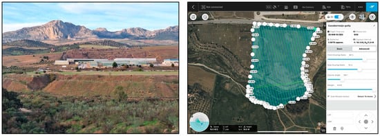
Figure 1.
Landscape overview (left) and flight planification using DJI GS Pro (right).
2.2. Drone Characteristics and Flight Planification
We used a DJI Mavic 2 Enterprise Zoom for this study. Its optical zoom capability was useful for identifying detailed features. The DJI Mavic 2 Enterprise Zoom is a professional UAV weighing 905 g, with a maximum flight time of 31 min. It can reach speeds of up to 72 km/h, operate at altitudes up to 6000 m, and withstand winds up to 38 km/h. Its camera features a 2× optical zoom, 3× digital zoom, 4 K video at 30 fps, and a 1/2.3” 12 MP CMOS sensor, ensuring high-quality imaging. Its compact, foldable design enhances portability and efficiency to assess land degradation processes after extreme events. The flight was conducted on 4 October 2024, using the DJI GS Pro software (v2.0.17), which lasted 36 min and 55 s and captured a total of 840 photographs (Figure 2). This software streamlines DJI drone operations through automated flight missions, cloud-based data management, and collaborative project features, enabling efficient planning, data handling, and team collaboration for diverse drone applications.
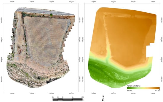
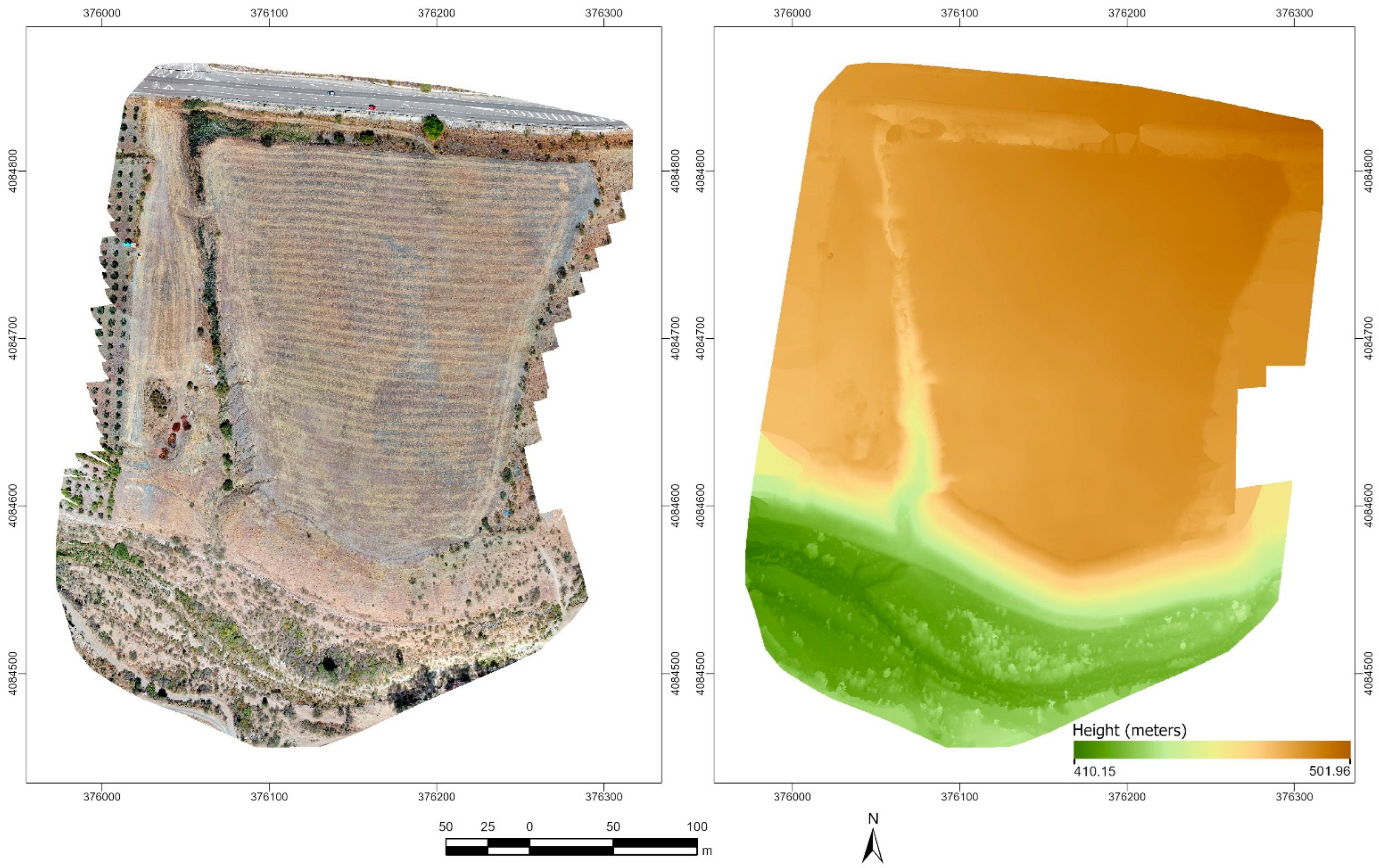
Figure 2.
Orthomosaic (left) and Digital Surface Model (right).
Previously, we incorporated 24 ground control points (GCPs) for accurate georeferencing using a Reach RS+ receiver (EMLID), an RTK GNSS single-band device. Although a single-frequency system, differential corrections from the Spanish National Geographic Institute (IGN) were applied through post-processing. This significantly improved positional accuracy, reducing the error to the centimeter level. The availability of high-quality RINEX data from IGN’s permanent reference stations allowed for precise georeferencing despite the inherent hardware limitations of single-band systems. Finally, Pix4D software (Version 1.78.0.) was used to adjust the digital model and orthophoto. Our flight operation involved the use of 3 batteries with a front overlap ratio set at 80%, a side overlap ratio of 70%, and a course angle of 103º. A total of 83 waypoints were executed across 36 lines, with a flight length of 9477 m, covering an area of 9.83 hectares. The shooting angle was perpendicular to the course, with capture mode at an equal distance, a speed of 5.1 m/s, and a shutter interval of 2 s, at an altitude of 35 m, resulting in a resolution of 1.3 cm/pixel.
2.3. Generation of Digital Surface Model (DSM) and Orthomosaic
We processed the image data captured during the flights using Pix4Dmapper software, a high-precision digital photogrammetry suite. First, we created a new project in Pix4Dmapper, importing all georeferenced images and ground control points (GCPs). This initial step set up the processing framework, including defining the coordinate system (WGS84 and EPGS 25380) and configuring project parameters. Next, the first processing stage involved key point extraction and image matching. This process identified common features in overlapping images, performed camera calibration, and conducted initial georeferencing, resulting in a sparse point cloud and camera positions. Reviewing the quality report generated after this stage was crucial to ensure the accuracy of image matching. The second stage focused on generating a dense point cloud and a 3D mesh. Here, advanced algorithms densified the point cloud, creating a detailed three-dimensional representation of the study area. Subsequently, a 3D mesh was generated by connecting these dense points, forming a continuous surface.
The third and final processing stage involved generating the Digital Surface Model (DSM) and the orthomosaic with a resolution of 1.3 cm. The DSM was created as a raster representing the surface elevation, while the orthomosaic was generated as a georeferenced and orthorectified image, free from geometric distortions. Both products underwent a thorough quality review using Pix4Dmapper’s editing tools to correct any errors or artifacts. Finally, the DSM and the orthomosaic were exported in GeoTIFF formats for further analysis in QGIS software (v. 3.42.3), enabling the extraction of detailed and accurate topographic information (Figure 2).
To enhance the georeferencing accuracy of our drone imagery, we used a rigorous alignment process. This involved utilizing recent, high-resolution aerial orthophotographs provided by the Spanish National Aerial Orthophotography Plan (PNOA) of the National Geographic Institute (IGN) along with our GCPs. These up-to-date PNOA orthomosaics served as a reliable and authoritative reference dataset, spatially adjusting our UAV-derived data and ensuring a higher level of geometric precision than achievable with unreferenced drone imagery alone.
2.4. Designing Specific Steps for Smoothing and Vegetation Filter
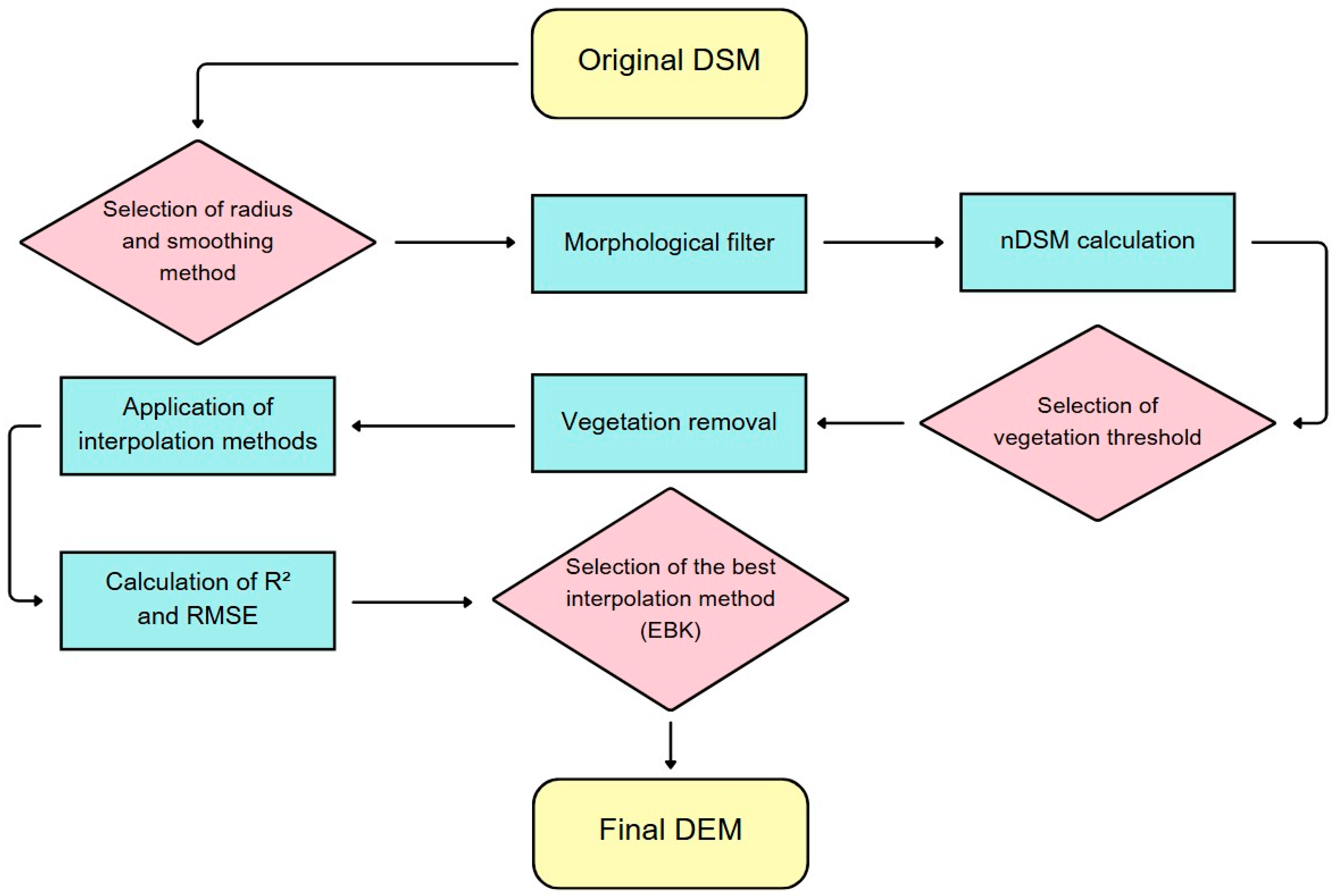
A step-by-step workflow and key parameters are provided in Figure 3 to support reproducibility. To remove vegetation from the DSM and generate a DEM, the process began with a smoothing step to reduce the influence of high-altitude values. This was achieved using the “Morphological filter” tool from the SAGA plugin in QGIS [40]. The selected method, “Opening,” applies two operations to each pixel within a defined neighborhood: first, “Erosion” assigns the minimum value found in the neighborhood, which reduces the prominence of small structures such as vegetation or buildings; then, “Dilation” assigns the maximum value within the same neighborhood, restoring the general terrain structure while suppressing sharp altitude variations. A smoothing radius of 50 pixels was defined. As verified through visual inspection, this radius allowed us to reduce the influence of vegetation without applying excessive smoothing that would remove too many terrain features. The result of this process is what we define as a “preliminary DEM,” as it reduces the impact of major vegetation features. However, additional steps were necessary to obtain a more accurate DEM for subsequent analyses (Figure 3). Using the preliminary DEM and the original DSM, we generated a Normalized Digital Surface Model (nDSM) by subtracting the DEM from the DSM [41]. This nDSM effectively highlights the tallest features, specifically the vegetation that was not fully smoothed out in the previous step [42].

Figure 3.
Workflow for converting a Digital Surface Model (DSM) to a Digital Elevation Model (DEM).
To obtain a more accurate, vegetation-free DEM, we then established a 1 m threshold to classify altitude values as vegetation. This means pixels where the difference between the DSM and the provisional DEM altitude values exceeded 1 m were considered vegetation and subsequently removed from the original DSM. This threshold was determined empirically through a combination of nDSM histogram analysis and visual inspection. We tested several thresholds (0.5 m, 1.0 m, 1.5 m), and 1 m proved the most effective. It offered an optimal balance, being high enough to identify and remove residual vegetation without affecting the underlying terrain, thus preserving natural landforms while eliminating vegetation not previously filtered. This step effectively removed all remaining traces of vegetation from the drone imagery.
2.5. Assessment of the Highest Statistical Significant Interpolation Methods
The final step in DEM generation involved filling the gaps left after vegetation removal through interpolation [43]. Several interpolation methods commonly used in scientific studies were tested in ArcGIS Pro, including Inverse Distance Weighting (IDW), different types of Kriging (Simple Kriging, Ordinary Kriging, Universal Kriging, and Empirical Bayesian Kriging), and Radial Basis Functions (Spline with Tension, Completely Regularized Spline, Multiquadric, and Inverse Multiquadric). Once the gaps were filled using these different methods, we evaluated their performance to determine the most suitable approach. For this, we calculated the R2 and Root Mean Square Error (RMSE) for each method.
3. Results
3.1. Smoothing and Vegetation Filter
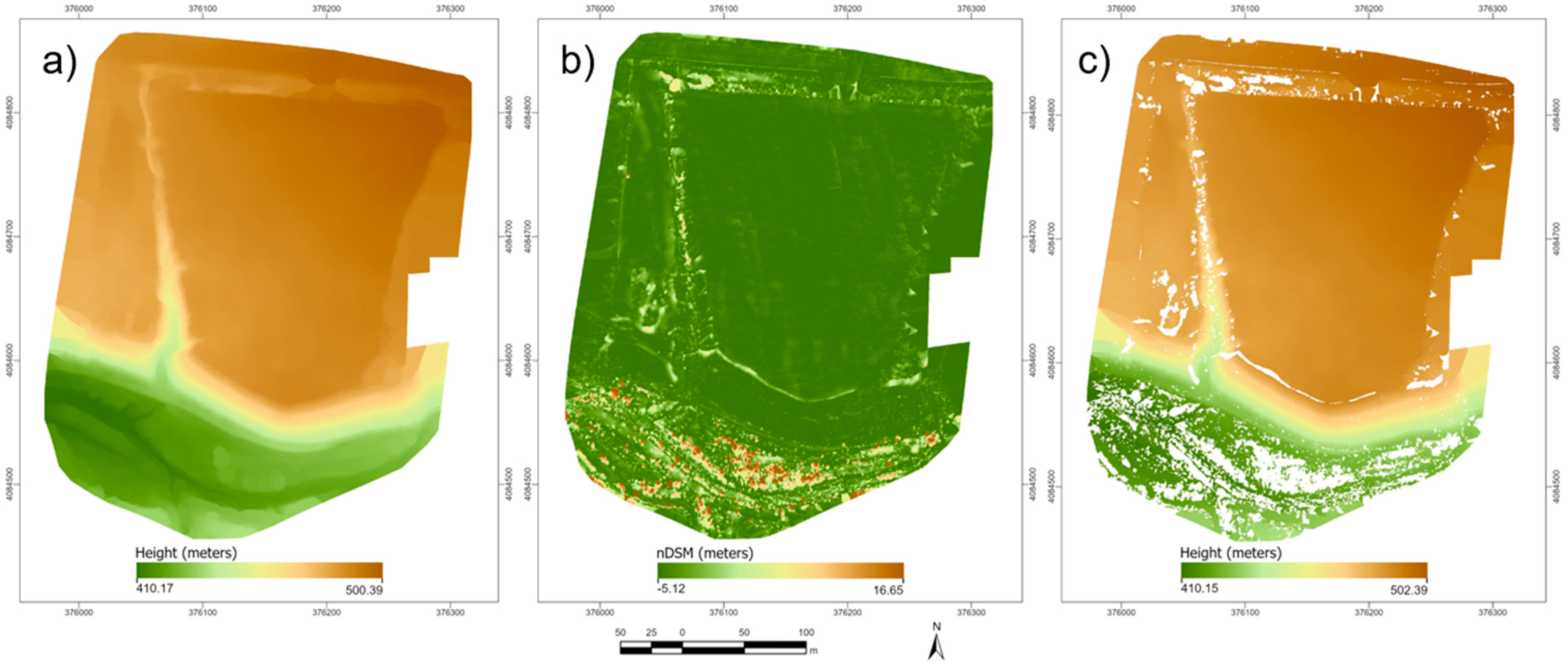
The provisional DEM resulting from the first smoothing step using the “Morphological filter” (Figure 4a) involved a reduction in the maximum altitude compared to the original DSM by 1.57 m (501.95 m for the DSM and 500.39 m for the provisional DEM) and the mean altitude by 0.45 m (469.99 m for the DSM and 469.54 m for the provisional DEM). In the visual result, the vegetation morphology that was visible in the original DSM is no longer apparent, but artificial circular patterns resulting from the smoothing can be identified. The subsequent nDSM (Figure 4b) accurately highlights the vegetation, which can be clearly identified in the orthophoto (Figure 2), although some small areas without vegetation are also highlighted. This calculation identified altitude differences between the initial DSM and the provisional DEM of up to 16.65 m in some pixels, as shown in the map. However, the average nDSM value is 0.44 m in altitude. The vegetation removal resulting from the threshold selected from this nDSM (Figure 4c) led to a reduction of 1.23 ha of terrain (12.5%). As shown in Figure 1 and Figure 2, the filtering process effectively removed small shrubs and riparian vegetation.

Figure 4.
Smoothing and filter application procedures. (a) Result of the morphological filter; (b) Normalized Digital Surface Model (nDSM); (c) result after vegetation removal.
After calculating the RMSE and R2 for all the interpolation methods applied to fill the gaps left by the removed vegetation (Table 1), the method that resulted in the lowest RMSE and highest R2 values was Empirical Bayesian Kriging (EBK). Then, various Radial Basis Function methods, including IDW, with the other types of Kriging methods at the bottom.

Table 1.
RMSE and R2 values of the interpolation methods used.
3.2. Interpolation Methods
Regarding the visual result of the final DEM compared to the initial DSM (Figure 5), the absence of the vegetation morphology is noticeable, and compared to the DEM resulting from the morphological filter (Figure 4), there is a much less artificial surface across the study area, leading to a more accurate representation of the ground surface. In terms of statistical differences between the two models (Table 2), the reduction in both the mean and maximum altitudes stands out, specifically by 0.25 and 0.45 m (the latter value also corresponds to the reduction in range). Compared to the difference between the original DSM and the provisional DEM resulting from the morphological filter, the difference in mean altitudes is the same, but the difference in maximum altitudes is much smaller in the case of the final DEM. It is also noteworthy that the standard deviation in the final DEM has increased compared to the initial DSM.
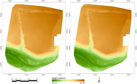
Figure 5.
Visual comparison between the original DSM (left) and the final DEM (right).
Table 2.
Statistical comparison between the original DSM and the final DEM.
Analyzing the differences between the distributions of the original DSM and the final DEM (Figure 6a), we can observe that lower altitude values are more frequent in the final DEM, and the opposite is true for higher values, which are more frequent in the original DSM, due to the absence of vegetation in the DEM. The frequency of intermediate values is similar in both. Regarding the scatter plots, in the first one, where the altitude values of the DSM and the DEM are differentiated by color (Figure 6b), the greater differences we observed in their distributions stand out, corresponding to a higher number of lower values in the DEM. In the second scatter plot, where the cases where DSM values are higher than the DEM values and vice versa are differentiated by color (Figure 6c), what stands out most is the higher frequency of cases where the DSM altitude is higher than the DEM, which is logical due to the removal of vegetation, which corresponded to a higher altitude, especially in the higher values, where the superiority of the DEM values over the DSM is very rare.
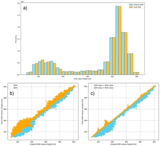
Figure 6.
Statistical comparison of DSM (Digital Surface Model) and DEM (Digital Elevation Model). (a) Histogram of DSM and DEM; (b) scatter plot for identifying DSM and DEM values; (c) scatter plot showing the relationship between DSM and DEM values.
Once we had established the methodology to apply it to other flights, we generated preliminary terrain maps using the DEM from this flight (Figure 7). These maps highlight various terrain features of the study area, which will be analyzed in greater depth in subsequent studies, in which we aim to assess temporal changes in the terrain by comparing two key moments: pre-DANA (represented in the current maps) and post-DANA. The DANA refers to a meteorological phenomenon characterized by extreme rainfall events that affected several regions of Spain. These maps and analyses will be used to explore the impact of DANA on the study area, focusing on the terrain changes before and after the event.
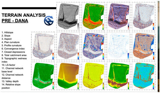
Figure 7.
Geomorphological maps generated using SAGA software (v. 9).
4. Discussion
This paper aimed to address the limitations in geomorphological mapping when access to LiDAR, public, or remote sensing data is restricted. It offers a viable methodology to achieve a minimum quality standard under such constraints. Furthermore, it seeks to present a valuable option for rapid landscape assessment following extreme events like Mediterranean storms, thereby demonstrating a practical approach for timely environmental monitoring in critical situations. The methodology presented in this study successfully converted a Digital Surface Model (DSM) to a Digital Elevation Model (DEM) using an RGB camera. This was achieved by employing a combination of morphological filtering, threshold-based vegetation removal, and interpolation. Visual inspection of the final DEM confirmed the effective removal of vegetation features and demonstrated that the smoothing process did not excessively generalize the terrain. Furthermore, the statistical analysis of the interpolation methods, particularly Empirical Bayesian Kriging (EBK), revealed high accuracy with a low Root Mean Square Error (RMSE) of 0.037 and a high R2 of 0.999993. This indicates a robust and reliable conversion process.
The integration of drone technology and advanced computational image analysis has revolutionized geomorphological studies, offering unprecedented benefits [44]. Drones enable the rapid acquisition of high-resolution spatial data, capturing detailed topographic features that were previously inaccessible or time-consuming to survey. Coupled with sophisticated image processing algorithms, such as those used for DEM generation, these data facilitate precise mapping and analysis of landforms [45]. Computational advancements allow for the efficient handling of large datasets, enabling the extraction of subtle geomorphological features and the creation of accurate 3D models [46]. This synergy enhances our ability to monitor dynamic processes like erosion, landslides, and fluvial changes, providing valuable insights for hazard assessment, resource management, and understanding of Earth’s surface evolution [47].
We acknowledge that our approach of filtering vegetation solely within the DEM might present certain limitations. While we aimed to explore the feasibility and potential of this specific approach for efficient vegetation removal in certain contexts, we recognize that it may not be suitable for all applications and could introduce inaccuracies that would be better addressed by incorporating point cloud information. Some weaknesses and potential areas for improvement were identified. Firstly, the threshold of 1 m used for vegetation removal inadvertently eliminated some higher-altitude terrain features devoid of vegetation. This highlights a potential limitation of relying solely on a fixed threshold, as it may lead to over-homogenization of the terrain and the loss of critical topographic details, despite the high resolution of the drone imagery. This underscores the challenge of balancing vegetation removal with the preservation of essential terrain characteristics. Secondly, the increase in the standard deviation in the final DEM compared to the original DSM was unexpected. Intuitively, removing higher altitude values associated with vegetation should have resulted in a decrease in standard deviation. The observed increase suggests that the interpolation process and the removal of certain data points may have introduced greater variability in the remaining terrain surface. Further investigation into the spatial distribution of these variations is warranted to fully understand this phenomenon, which has been debated for many years [48,49]. Thirdly, the methodology involved a significant amount of manual parameter tuning, which can be time-consuming and subjective. The reliance on visual inspection and iterative adjustments makes the process potentially lengthy and prone to variability depending on the operator. This suggests a need for more automated or adaptive methods to streamline the workflow and reduce subjectivity [50,51].
The visual assessment confirmed the effective removal of vegetation without excessive smoothing, maintaining a realistic representation of the terrain. Statistically, the interpolation results were accurate, particularly with EBK and the Multiquadric Radial Basis Function method, which showed minimal differences in performance. The generalizability of this methodology to other study areas by adjusting parameters is also a significant advantage. To further enhance the accuracy and reliability of the final DEM, several improvements can be considered. Most importantly, validating the DEM with field-collected data would provide a crucial assessment of its accuracy [52,53]. This validation could involve comparing the DEM elevations with under-vegetation ground control points or LiDAR data. Additionally, exploring adaptive thresholding techniques or machine learning algorithms for vegetation classification could potentially reduce the over-homogenization of the terrain [54,55]. Developing more automated parameter optimization methods could also significantly streamline the workflow and reduce subjectivity.
Compared to existing approaches, the proposed methodology offers several notable advantages: it enables the generation of accurate DEMs in vegetated areas without the need for LiDAR sensors, significantly reducing costs and simplifying logistics for first approaches. Despite relying solely on RGB imagery, the method achieved high accuracy, with a very low RMSE and a high R2, particularly using Empirical Bayesian Kriging interpolation. Furthermore, the approach is adaptable to other study areas through parameter adjustment, making it versatile and reproducible. Although it currently involves some manual parameter tuning, the workflow lays the groundwork for future improvements based on automation or machine learning algorithms, enhancing its potential for cost-effective, high-resolution geomorphological studies.
5. Conclusions
This study demonstrated a methodology for converting a DSM to a DEM using a combination of morphological filtering, threshold-based vegetation removal, and interpolation from an RGB camera, and without ground control points. The final DEM effectively removed vegetation features while maintaining a realistic representation of the terrain, as confirmed by visual inspection. The statistical analysis of the interpolation methods highlighted the high accuracy of the Empirical Bayesian Kriging (EBK) method, which yielded the lowest RMSE and highest R2 values. However, the study also revealed some limitations. The use of a fixed threshold for vegetation removal led to the unintentional removal of some non-vegetated terrain features, highlighting the challenge of balancing vegetation removal with terrain preservation. Additionally, the increase in standard deviation in the final DEM compared to the original DSM was unexpected and warrants further investigation. The manual parameter tuning involved in the methodology also presents a potential source of subjectivity and time consumption.
Despite these limitations, the methodology offers a valuable approach to DEM generation, particularly in areas with dense vegetation. The high accuracy of the interpolation results and the generalizability of the methodology to other study areas are significant strengths. Future improvements, such as the incorporation of field validation data and the development of more automated parameter optimization methods, could further enhance the accuracy and efficiency of the DEM generation process. The integration of drone technology and advanced computational image analysis holds great promise for geomorphological studies, enabling the efficient and accurate mapping and analysis of landforms.
Author Contributions
Conceptualization, J.R.-C.; methodology, M.T.G.-M. and J.R.-C.; validation, M.T.G.-M. and J.R.-C.; formal analysis, M.T.G.-M. and J.R.-C.; investigation, M.T.G.-M. and J.R.-C.; data curation, M.T.G.-M.; writing—original draft preparation, M.T.G.-M. and J.R.-C.; writing—review and editing, M.T.G.-M. and J.R.-C.; visualization, M.T.G.-M. and J.R.-C.; supervision, J.R.-C.; project administration, J.R.-C.; funding acquisition, J.R.-C. All authors have read and agreed to the published version of the manuscript.
Funding
This research was funded by the Ministerio de Ciencia, Innovación y Universidades, under the project titled “Desarrollo de productos basados en los nuevos sensores satelitales hiperespectrales europeos e ia para la caracterizacion de estresores en tierras de cultivo (HIPROESTRES)” (grant number PID2023-152656OB-I00), within the Programa Estatal de Investigación Científica, Técnica y de Innovación (2021–2023).
Data Availability Statement
Data will be shared upon request.
Conflicts of Interest
The authors declare no conflicts of interest.
References
- Viles, H. Technology and Geomorphology: Are Improvements in Data Collection Techniques Transforming Geomorphic Science? Geomorphology 2016, 270, 121–133. [Google Scholar] [CrossRef]
- Rodrigo-Comino, J.; Keesstra, S.D.; Cerdà, A. Updating the Scientific Content of the Modern Geography of Viticulture for Human, Physical and Regional Applied Studies. Mediterr. Geosci. Rev. 2024, 6, 111–121. [Google Scholar] [CrossRef]
- Chen, H.-W.; Chen, C.-Y.; Yang, P.-Z. Using Drone-Based Multispectral Imaging for Investigating Gravelly Debris Flows and Geomorphic Characteristics. Environ. Earth Sci. 2024, 83, 247. [Google Scholar] [CrossRef]
- Mirzaee, S.; Pajouhesh, M.; Imaizumi, F.; Abdollahi, K.; Gomez, C. Gully Erosion Development during an Extreme Flood Event Using UAV Photogrammetry in an Arid Area, Iran. CATENA 2024, 246, 108347. [Google Scholar] [CrossRef]
- Mirzaee, S.; Gomez, C.; Pajouhesh, M.; Abdollahi, K. Chapter 16—Soil Erosion and Sediment Change Detection Using UAV Technology. In Remote Sensing of Soil and Land Surface Processes; Melesse, A.M., Rahmati, O., Khosravi, K., Petropoulos, G.P., Eds.; Earth Observation; Elsevier: Amsterdam, The Netherlands, 2024; pp. 271–279. ISBN 978-0-443-15341-9. [Google Scholar]
- Zhang, J.; Guo, W.; Zhou, B.; Okin, G.S. Drone-Based Remote Sensing for Research on Wind Erosion in Drylands: Possible Applications. Remote Sens. 2021, 13, 283. [Google Scholar] [CrossRef]
- Riddle, L.; Hill, T.; Gijsbertsen, B. Geomorphology from ‘on High’: The Use of Drones/ UAV Technology in Teaching Soil Erosion. J. Geogr. Educ. Afr. 2021, 4, 58–74. [Google Scholar] [CrossRef]
- Takata, Y.; Yamada, H.; Kanuma, N.; Ise, Y.; Kanda, T. Digital Soil Mapping Using Drone Images and Machine Learning at the Sloping Vegetable Fields in Cool Highland in the Northern Kanto Region, Japan. Soil Sci. Plant Nutr. 2023, 69, 221–230. [Google Scholar] [CrossRef]
- Xie, X.; Duan, W.; Yin, Z.; Duan, W.; Bu, J.; Lu, Y. Identification Method of Regional Soil Erosion Characteristics Based on Drone Low Altitude Remote Sensing Technology. In Proceedings of the Fifth International Conference on Geology, Mapping, and Remote Sensing (ICGMRS 2024), Wuhan, China, 12–14 April 2024; SPIE: Bellingham, WA, USA, 2024; Volume 13223, pp. 97–102. [Google Scholar]
- Cândido, B.M.; James, M.; Quinton, J.; Lima, W.d.; Silva, M.L.N. Sediment Source and Volume of Soil Erosion in a Gully System Using UAV Photogrammetry. Rev. Bras. Ciênc. Solo 2020, 44, e0200076. [Google Scholar] [CrossRef]
- Carabassa, V.; Montero, P.; Alcañiz, J.M.; Padró, J.-C. Soil Erosion Monitoring in Quarry Restoration Using Drones. Minerals 2021, 11, 949. [Google Scholar] [CrossRef]
- Mei, A.; Ragazzo, A.V.; Rantica, E.; Fontinovo, G. Statistics and 3D Modelling on Soil Analysis by Using Unmanned Aircraft Systems and Laboratory Data for a Low-Cost Precision Agriculture Approach. AgriEngineering 2023, 5, 1448–1468. [Google Scholar] [CrossRef]
- Xiao, W.; Ren, H.; Sui, T.; Zhang, H.; Zhao, Y.; Hu, Z. A Drone- and Field-Based Investigation of the Land Degradation and Soil Erosion at an Opencast Coal Mine Dump after 5 Years’ Evolution of Natural Processes. Int. J. Coal Sci. Technol. 2022, 9, 42. [Google Scholar] [CrossRef]
- Ruwaimana, M.; Satyanarayana, B.; Otero, V.; Muslim, A.M.; Syafiq A, M.; Ibrahim, S.; Raymaekers, D.; Koedam, N.; Dahdouh-Guebas, F. The Advantages of Using Drones over Space-Borne Imagery in the Mapping of Mangrove Forests. PLoS ONE 2018, 13, e0200288. [Google Scholar] [CrossRef]
- Mohd Noor, N.; Abdullah, A.; Hashim, M. Remote Sensing UAV/Drones and Its Applications for Urban Areas: A Review. IOP Conf. Ser. Earth Environ. Sci. 2018, 169, 012003. [Google Scholar] [CrossRef]
- Bansod, B.; Singh, R.; Thakur, R.; Singhal, G. A Comparision between Satellite Based and Drone Based Remote Sensing Technology to Achieve Sustainable Development: A Review. J. Agric. Environ. Int. Dev. 2017, 111, 383–407. [Google Scholar] [CrossRef]
- Inoue, Y. Satellite- and Drone-Based Remote Sensing of Crops and Soils for Smart Farming—A Review. Soil Sci. Plant Nutr. 2020, 66, 798–810. [Google Scholar] [CrossRef]
- Gray, P.C.; Ridge, J.T.; Poulin, S.K.; Seymour, A.C.; Schwantes, A.M.; Swenson, J.J.; Johnston, D.W. Integrating Drone Imagery into High Resolution Satellite Remote Sensing Assessments of Estuarine Environments. Remote Sens. 2018, 10, 1257. [Google Scholar] [CrossRef]
- Alsamarraie, M.; Ghazali, F.; Hatem, Z.M.; Flaih, A.Y. A Review on the Benefits, Barriers of the Drone Employment in the Construction Site. J. Teknol. Sci. Eng. 2022, 84, 121–131. [Google Scholar] [CrossRef]
- Pensado, E.A.; Carrera, G.F.; López, F.V.; Jorge, H.G.; Ortega, E.M. Turbulence-Aware UAV Path Planning in Urban Environments. In Proceedings of the 2024 International Conference on Unmanned Aircraft Systems (ICUAS), Chania, Greece, 4–7 June 2024; pp. 280–285. [Google Scholar]
- Gao, M.; Hugenholtz, C.H.; Fox, T.A.; Kucharczyk, M.; Barchyn, T.E.; Nesbit, P.R. Weather Constraints on Global Drone Flyability. Sci. Rep. 2021, 11, 12092. [Google Scholar] [CrossRef] [PubMed]
- Thibbotuwawa, A.; Bocewicz, G.; Radzki, G.; Nielsen, P.; Banaszak, Z. UAV Mission Planning Resistant to Weather Uncertainty. Sensors 2020, 20, 515. [Google Scholar] [CrossRef]
- Jeong, N.; Hwang, H.; Matson, E.T. Evaluation of Low-Cost LiDAR Sensor for Application in Indoor UAV Navigation. In Proceedings of the 2018 IEEE Sensors Applications Symposium (SAS), Seoul, Republic of Korea, 12–14 March 2018; pp. 1–5. [Google Scholar]
- Risbøl, O.; Gustavsen, L. LiDAR from Drones Employed for Mapping Archaeology—Potential, Benefits and Challenges. Archaeol. Prospect. 2018, 25, 329–338. [Google Scholar] [CrossRef]
- Kellner, J.R.; Armston, J.; Birrer, M.; Cushman, K.C.; Duncanson, L.; Eck, C.; Falleger, C.; Imbach, B.; Král, K.; Krůček, M.; et al. New Opportunities for Forest Remote Sensing Through Ultra-High-Density Drone Lidar. Surv. Geophys. 2019, 40, 959–977. [Google Scholar] [CrossRef] [PubMed]
- Hout, R.; Maleval, V.; Mahe, G.; Rouvellac, E.; Crouzevialle, R.; Cerbelaud, F. UAV and LiDAR Data in the Service of Bank Gully Erosion Measurement in Rambla de Algeciras Lakeshore. Water 2020, 12, 2748. [Google Scholar] [CrossRef]
- Niculiță, M.; Mărgărint, M.C.; Tarolli, P. Chapter 10—Using UAV and LiDAR Data for Gully Geomorphic Changes Monitoring. In Developments in Earth Surface Processes; Tarolli, P., Mudd, S.M., Eds.; Remote Sensing of Geomorphology; Elsevier: Amsterdam, The Netherlands, 2020; Volume 23, pp. 271–315. [Google Scholar]
- Tak, W.J.; Jun, K.W.; Kim, S.D.; Lee, H.J. Using Drone and LiDAR to Assess Coastal Erosion and Shoreline Change due to the Construction of Coastal Structures. J. Coast. Res. 2020, 95, 674–678. [Google Scholar] [CrossRef]
- Skarlatos, D.; Vlachos, M. Vegetation removal from uav derived dsms, using combination of rgb and nir imagery. ISPRS Ann. Photogramm. Remote Sens. Spat. Inf. Sci. 2018, IV-2, 255–262. [Google Scholar] [CrossRef]
- Anders, N.; Valente, J.; Masselink, R.; Keesstra, S. Comparing Filtering Techniques for Removing Vegetation from UAV-Based Photogrammetric Point Clouds. Drones 2019, 3, 61. [Google Scholar] [CrossRef]
- Pirotti, F.; Guarnieri, A.; Vettore, A. State of the Art of Ground and Aerial Laser Scanning Technologies for High-Resolution Topography of the Earth Surface. Eur. J. Remote Sens. 2013, 46, 66–78. [Google Scholar] [CrossRef]
- Senciales González, J.M.; Rodrigo Comino, J. Geomorfología de Los Montes de Málaga: Pasado, Presente y ¿futuro? BAÉTICA Estud. Arte Geogr. Historia 2011, 33, 81–109. [Google Scholar] [CrossRef]
- Martínez Murillo, J.F.; Ruiz Sinoga, J.D. Incidencia de Algunas Propiedades Físicas de Suelos En Su Respuesta Hidrológica Ante Diferentes Usos Bajo Condiciones Mediterráneas (Montes de Málaga). Edafología 2003, 10, 57–62. [Google Scholar]
- Martínez Murillo, J.F.; Senciales González, J.M. Morfogénesis y Procesos Edáficos: El Caso de Los Montes de Málaga. BAÉTICA Estud. Arte Geogr. Historia 2003, 25, 219–258. [Google Scholar]
- Rodrigo-Comino, J. Los Suelos de la Provincia de Málaga: Revisión y Actualización de las Fuentes Edafológicas Según la Clasificación de FAO-WRB; Servicio de Publicaciones y Divulgación Científica, Universidad de Málaga: Málaga, Spain, 2014; ISBN 978-84-9747-880-9. [Google Scholar]
- IUSS-WRB Base for Soil Resources. International Soil Classification System for Naming Soils and Creating Legends for Soil Maps, 4th ed.; International Union of Soil Sciences (IUSS): Vienna, Austria, 2022. [Google Scholar]
- Medina, J.A.S.; Sinoga, J.D.R.; Medina, J.A.S.; Sinoga, J.D.R. La Cuenca del Río Guadalmedina: Peligrosidad Frente a la Erosión Hídrica; UMA Editorial: Málaga, Spain, 2023; ISBN 978-84-13-35251-0. [Google Scholar]
- Valsero, J.J.D. Atlas Hidrogeológico de la Provincia de Málaga; IGME: Madrid, Spain, 2007; ISBN 978-84-7840-675-3. [Google Scholar]
- Rodrigo-Comino, J.; Senciales, J.M.; Sillero-Medina, J.A.; Gyasi-Agyei, Y.; Ruiz-Sinoga, J.D.; Ries, J.B. Analysis of Weather-Type-Induced Soil Erosion in Cultivated and Poorly Managed Abandoned Sloping Vineyards in the Axarquía Region (Málaga, Spain). Air Soil Water Res. 2019, 12, 1178622119839403. [Google Scholar] [CrossRef]
- Passy, P.; Théry, S. The Use of SAGA GIS Modules in QGIS. In QGIS and Generic Tools; John Wiley & Sons, Ltd.: Hoboken, NJ, USA, 2018; pp. 107–149. ISBN 978-1-119-45709-1. [Google Scholar]
- Yeom, J.; Lee, W.; Kim, T.; Han, Y. Normalized Digital Surface Model Extraction and Slope Parameter Determination through Region Growing of UAV Data. J. Korean Soc. Surv. Geod. Photogramm. Cartogr. 2019, 37, 499–506. [Google Scholar] [CrossRef]
- Zimmermann, S.; Hoffmann, K. Accuracy Assessment of Normalized Digital Surface Models from Aerial Images Regarding Tree Height Determination in Saxony, Germany. PFG 2017, 85, 257–263. [Google Scholar] [CrossRef]
- Polidori, L.; El Hage, M. Digital Elevation Model Quality Assessment Methods: A Critical Review. Remote Sens. 2020, 12, 3522. [Google Scholar] [CrossRef]
- Mitra, S.; Pundir, S.; Devrani, R.; Arora, A.; Pandey, M.; Costache, R.; Janizadeh, S. An Overview of Morphometry Software Packages, Tools, and Add-Ons. In Advances in Remote Sensing Technology and the Three Poles; John Wiley & Sons, Ltd.: Hoboken, NJ, USA, 2022; pp. 49–57. ISBN 978-1-119-78775-4. [Google Scholar]
- Katzil, Y.; Doytsher, Y. Height Estimation Methods for Filling Gaps in Gridded DTM. J. Surv. Eng. 2000, 126, 145–162. [Google Scholar] [CrossRef]
- Gavriil, K.; Muntingh, G.; Barrowclough, O.J.D. Void Filling of Digital Elevation Models with Deep Generative Models. IEEE Geosci. Remote Sens. Lett. 2019, 16, 1645–1649. [Google Scholar] [CrossRef]
- Yurish, S. Drones and Unmanned Systems. In Proceedings of the 1st International Conference on Drones and Unmanned Systems (DAUS’ 2025), Granada, Spain, 19–21 February 2025. [Google Scholar]
- Erdogan, S. A Comparision of Interpolation Methods for Producing Digital Elevation Models at the Field Scale. Earth Surf. Process. Landf. 2009, 34, 366–376. [Google Scholar] [CrossRef]
- Chaplot, V.; Darboux, F.; Bourennane, H.; Leguédois, S.; Silvera, N.; Phachomphon, K. Accuracy of Interpolation Techniques for the Derivation of Digital Elevation Models in Relation to Landform Types and Data Density. Geomorphology 2006, 77, 126–141. [Google Scholar] [CrossRef]
- Li, S.; Hu, G.; Cheng, X.; Xiong, L.; Tang, G.; Strobl, J. Integrating Topographic Knowledge into Deep Learning for the Void-Filling of Digital Elevation Models. Remote Sens. Environ. 2022, 269, 112818. [Google Scholar] [CrossRef]
- Li, S.; Xiong, L.; Tang, G.; Strobl, J. Deep Learning-Based Approach for Landform Classification from Integrated Data Sources of Digital Elevation Model and Imagery. Geomorphology 2020, 354, 107045. [Google Scholar] [CrossRef]
- Polidori, L.; El Hage, M.; Valeriano, M.D.M. Digital Elevation Model Validation with No Ground Control: Application to the Topodata Dem in Brazil. Bol. Ciênc. Geod. 2014, 20, 467–479. [Google Scholar] [CrossRef]
- Murphy, P.N.C.; Ogilvie, J.; Meng, F.-R.; Arp, P. Stream network modelling using lidar and photogrammetric digital elevation models: A comparison and field verification. Hydrol. Process. 2008, 22, 1747–1754. [Google Scholar] [CrossRef]
- Bae, J.H.; Han, J.; Lee, D.; Yang, J.E.; Kim, J.; Lim, K.J.; Neff, J.C.; Jang, W.S. Evaluation of Sediment Trapping Efficiency of Vegetative Filter Strips Using Machine Learning Models. Sustainability 2019, 11, 7212. [Google Scholar] [CrossRef]
- Pan, W.; Wang, X.; Sun, Y.; Wang, J.; Li, Y.; Li, S. Karst Vegetation Coverage Detection Using UAV Multispectral Vegetation Indices and Machine Learning Algorithm. Plant Methods 2023, 19, 7. [Google Scholar] [CrossRef] [PubMed]


Disclaimer/Publisher’s Note: The statements, opinions and data contained in all publications are solely those of the individual author(s) and contributor(s) and not of MDPI and/or the editor(s). MDPI and/or the editor(s) disclaim responsibility for any injury to people or property resulting from any ideas, methods, instructions or products referred to in the content. |
© 2025 by the authors. Licensee MDPI, Basel, Switzerland. This article is an open access article distributed under the terms and conditions of the Creative Commons Attribution (CC BY) license (https://creativecommons.org/licenses/by/4.0/).