Article

Three Hundred and Sixty Degree Real-Time Monitoring of 3-D Printing Using Computer Analysis of Two Camera Views

by
Siranee Nuchitprasitchai
1,
Michael C. Roggemann
1 and
Joshua M. Pearce
2,*
1
Department of Electrical & Computer Engineering, Michigan Technological University, Houghton, MI 49931, USA
2
Department of Materials Science & Engineering, Michigan Technological University, Houghton, MI 49931, USA
*
Author to whom correspondence should be addressed.
J. Manuf. Mater. Process. 2017, 1(1), 2; https://doi.org/10.3390/jmmp1010002
Submission received: 15 May 2017 / Revised: 19 June 2017 / Accepted: 22 June 2017 / Published: 4 July 2017

Abstract

:
Prosumer (producing consumer)-based desktop additive manufacturing has been enabled by the recent radical reduction in 3-D printer capital costs created by the open-source release of the self-replicating rapid prototype (RepRap). To continue this success, there have been some efforts to improve reliability, which are either too expensive or lacked automation. A promising method to improve reliability is to use computer vision, although the success rates are still too low for widespread use. To overcome these challenges an open source low-cost reliable real-time optimal monitoring platform for 3-D printing from double cameras is presented here. This error detection system is implemented with low-cost web cameras and covers 360 degrees around the printed object from three different perspectives. The algorithm is developed in Python and run on a Raspberry Pi3 mini-computer to reduce costs. For 3-D printing monitoring in three different perspectives, the systems are tested with four different 3-D object geometries for normal operation and failure modes. This system is tested with two different techniques in the image pre-processing step: SIFT and RANSAC rescale and rectification, and non-rescale and rectification. The error calculations were determined from the horizontal and vertical magnitude methods of 3-D reconstruction images. The non-rescale and rectification technique successfully detects the normal printing and failure state for all models with 100% accuracy, which is better than the single camera set up only. The computation time of the non-rescale and rectification technique is two times faster than the SIFT and RANSAC rescale and rectification technique.

1. Introduction

Prosumer (producing consumer) based additive manufacturing has been enabled by the recent radical reduction in 3-D printer capital costs [1] created by the open-source release of the self-replicating rapid prototyper (RepRap) [2,3,4]. The open-source hardware approach [5] has followed the traditional rapid development seen in free and open source software [6] and the top-desktop 3-D printers are now routinely open source RepRap derivatives [7]. The fast growth of the RepRap 3-D printers is a result of their ability to replicate (e.g., print their own parts) and self-upgrade its own parts (e.g., print a new cooling fan duct) as well as their ability to easily pay for themselves by fabricating consumer goods [8,9]. In addition, open source desktop 3-D printers have been applied to create high-value items in a wide range of fields including: rapid prototyping [10,11], distributed manufacturing [12,13], education [14,15,16], sustainable technology [17,18,19], scientific tools [20,21,22,23], microfluidics [24,25].
Despite this success, these low-cost 3-D printers still suffer from a litany of printing challenges related to building up a part from thermoplastic one layer at time from a flat print bed including warping, elephant foot (thicker part touching the print bed), bed adhesion (prints peeling off of the bed during print), distortion due to shrinking, skewed prints/shifted layers, layer misalignment, clogged nozzles, or snapped filament [10,24,26]. These unintended results reduce the economic as well as the environmental advantage of distributed manufacturing with 3-D printing [20,21,27,28,29] in the aspect of environmental and sustainability. Many works have been undertaken to automatically detect the errors while printing, but most of them are for the expensive laser-based 3-D printing [30,31,32,33]. Therefore, there is an acute need for a low-cost real-time error detection system for prosumer-grade 3-D printers.
There have been some efforts made to this end. There were several works detecting an error based on the laser and piezoelectric sensors, which are not easily adapted to the low-cost market [34,35,36]. A more promising method is to use computer vision, which has been shown to be highly effective at process monitoring for manufacturing [37,38,39,40,41,42,43,44,45,46,47,48]. Some previous works used cameras to monitor the 3-D printing process [49,50,51]. Hurd et al. installed Samsung Galaxy Tab 3 on the printer and monitored the printing via mobile phone [49] but this can monitor only the top view of the printed part. Therefore, horizontal size can be determined. Baumann et al. used OpenCV [52], Python [53], and a PlayStation eye cam to detect detachment, missing material flow and deformed object in 3-D printing [50], however, this work can detect only the shape of the printed part from only one side with success rate of 80%. Straub successfully applied a visible light 3-D scanning system, five Raspberry Pi cameras, Raspberry Pi [54], and open source software approach with C# and Dot Net Framework [55] to detect incomplete prints [51]. Nonetheless, the work can only detect error in the shape aspect. Other solutions to detect the failure 3-D printing in the RepRap 3-D printer have had a video monitor of printing but the user must manually check the video and stop the printing if something goes wrong [56,57,58,59,60].
To monitor errors during FFF-based 3-D printing, an open source low-cost reliable real-time optimal monitoring platform for FFF-based 3-D printing from double cameras is presented here. This error detection system is implemented with low-cost web cameras and extended from the basic approaches dis-cussed above for 360 degrees around the printed object from three different perspectives by extending the algorithm using the Scale Invariant Feature Transform (SIFT) [61] and the Random Sample Consensus (RANSAC) [62] models previously described [63]. The algorithm is developed under open-source Python and run on a Raspberry Pi3 mini-computer to reduce the costs and computation time. For 3-D printing monitoring in three different perspectives, the systems are tested with four different 3-D object geometries (two experiments tested in the normal printing and two in the failure state). The normal printing state means that the filament can print correctly and complete printing the 3-D object. The failure state is the incomplete printing the 3-D object. This system is tested with two different techniques in the image pre-processing step: SIFT and RANSAC rescale and rectification, and non-rescale and rectification. The error percentage is calculated by the horizontal magnitude. Then the technique that can detect the error in the normal printing and the failure state will be used correctly in the second experiment where two different error detection methods are used: horizontal magnitude, and horizontal and vertical magnitudes. The results are discussed, conclusions are drawn and the limitations of these approaches are detailed.

2. Materials and Methods

2.1. Experimental Equipment

For this work, optical experiments were setup around a delta-style [64] RepRap as shown in Figure 1 running double cameras. This is a low-cost (<US $500 in parts) open source delta-style polymer printing RepRap (MOST Delta). The MOST Delta is a RepRap [65] derived from the Rostock [66] printer with a cylindrical build volume 270 mm in diameter and 250 mm high and overall dimensions of 375 mm diameter and 620 mm high. In addition, the STL and SCAD file are given for a first generation 3-D printable design to attach the cameras to the MOST delta [67]. The double camera error detection uses left and right images for three 3-D reconstructions (as seen in Figure 2). A Python algorithm was written for the experimental setup and is made available free and open source under an AGPLv3 license [63]. A different Python algorithm is used for each experimental setup, but the same type of webcam, 3-D printer, Raspberry Pi3, USB 3.0 hub with 12 V/3 A power adapter, three LED light sources, tested objects, black printing base, black background, and filament brand are used. Due to the distance between the camera and the printer for the experiment setup, the field of view for both cameras can cover the printed area of 70 mm in width and 60 mm in height. The relation of geometry between the 3-D printer and the camera system need to be known to be able to use the camera calibration technique [68] to calculate the intrinsic and extrinsic parameters for a specific camera setup. These parameters will be used to correct for lens distortion and image rectification. The three LED light sources [69] are installed on the three sides of the printer. All light sources are connected to the circuit with 4 volts from a DC power supply. The three pairs of cameras are set up on the same side of the LED light sources. All cameras are connected to a 7 port USB 3.0 hub with 12V/3A power adapter which is connected to Raspberry Pi3. The cameras used in this study are six Logitech C525 webcams, with an image size of 480-by-640 (height-by-width), pixel size is 5.52-by-5.82 μm (height-by-width), and a focal length of 39.5 mm. The pixel size and the focal length calculation of the webcam below.

2.2. Theory

2.2.1. Calculating Webcam Pixel Size and Focal Length

Unlike scientific cameras, inexpensive webcams do not normally ship with detailed technical specifications. The procedure below enables the extraction of pixel size and focal length from any inexpensive webcam. The Logitech C525 webcams used here do not come with information on the pixel size and focal length (on the package or the website), so the webcam was taken apart to calculate this information through the sensor size in the webcam as shown in Figure 3. The webcam sensor size is 2.52-by-3.73 mm (height-by-width), and the webcam diagonal is 4.50 mm. The width and the height of pixel size are calculated by
W d = W s / W i   ( μ m )
where W d is a width of pixel size ( μ m ), W s is the width of the sensor size (mm), and W i is the width of images size (pixels).
H p = H s / H i   ( μ m )
where H p is the height of pixel size ( μ m ), H s is the height of sensor size (mm), and H i is the height of images size (pixels).
The checkerboard image shown in Figure 4 is taken to calculate the focal length in pixels. The checkerboard image was printed in 2-D. The size of checkerboard square on paper is 7-by-7 mm [63]. The checkerboard image was taken where the distance between the image and the webcam was 230 mm, and the size of checkerboard square in the image was 20-by-20 pixels. The focal length in pixels is calculated by
F =   ( P * D ) / W c   ( pixels )
where F is the focal length (pixels), P is the size of checkerboard square in the image (pixels), D is the distance between the image and the webcam, and W c is the size of checkerboard square on the paper (pixels).
f =   ( F * W d ) / W i   ( mm )
where f is the focal length (mm), F is the focal length (pixels), W d is the width of pixel size ( μ m ), and W i is the width of images size (pixels).

2.2.2. Computer Vision Error Detection

There are three steps to prepare the error detection system before printing a 3-D model: (1) camera calibration, (2) preparing STereoLithography (STL) files and resultant images, and (3) setting up a pause and loop to move the extruder out of the view of the cameras for imaging. STL file is a file format describing 3-D model by using series of connected triangles to create the surface of the model and it is usually generated by computer-aided design (CAD) software. The first step is camera calibration. Sixteen chessboard (Figure 4) images are taken from three different views of the cameras after the 3-D printer experiment is setup for camera calibration. There are six cameras named as camera0, camera1, camera2, camera3, camera4, and camera5. The camera0 and camera1 are setup as the first pair of cameras, camera2 and camera3 are setup as the second pair, and camera4 and camera5 are setup as the third pair. The camera0, camera2, and the camera4 are setup as the left cameras, and camera1, camera 3, and the camera5 are setup as the right cameras. The calibration is calculated and saved as CalibrationData1, CalibrationData2, and CalibrationData3. The second step is preparing the stlimage by slicing stl files every N layers where the error will be detected as shown in Figure 5. The layer height and the amount of slicing layers need to be assigned for slicing stl file in three different views of the cameras. The layer height and the number of total layers can be found in gcode file. All data at every N layers from the stl file are plotted in x, y, z axes to display the shape of the rendered 3-D model, which can be observed from different viewpoints. The shape of the stlimage is saved as PNG image type on xz-plane. If a remainder after division between the total height and the height of every N layers is not equal to zero, the last PNG files are named as the amount of total layers. For example, if the 3-D model in gcode file has 129 total layers, layer height of 0.2 mm, and the 3-D model is slicing in every 30 layers, then the stl file is sliced at layer 30, 60, 90, 120, and 129 which result in heights of 6, 12, 18, 24, and 25.8 mm, respectively. The first stl slicing files are saved as SCAD30_1.png, SCAD30_2.png, and SCAD30_3.png, the next slicing files are saved as SCAD60_1.png, SCAD60_2.png, and SCAD60_3.png, and so on. After slicing stl files for four models, it was found that three stl files can start slicing every 10, 20, or 30 layers, but t55gear stl file can start slicing at every 30 layers. Therefore, this study will take six images every time 30 layers are printed. The last step in the process involves setting up a pause and a loop to move the extruder out of the images every N layers in order to eliminate visual noise in the object images, the extruder of 3-D printing will be paused and moved to the certain height. The 3-D model is designed in OpenSCAD version2015.03-3 (OpenSCAD, 2016) and it is rendered and saved into the stl file. After the 3-D model stl file is opened in Cura version15.04.6 (Ultimaker, 2016), the 3-D model is saved as gcode file. The 3-D model gcode file is opened by any text editor program to add the extra code in every N layers as shown in Figure 6.
The 3-D printing models chosen after the preparatory stlimage step are sun gear [70], prism, gear [71], and t55gear [72], which are available [73] as shown in Figure 7. The printing parameters used are: layer height 0.2 mm, shell thickness 1 mm, unable retraction, bottom/top thickness 1mm, fill density 20%, print speed 60 mm/s, printing temperature 180 °C, diameter filament 1.94–1.98 mm, flow filament 100%, and nozzle size 0.5 mm. The PLA filament used in this experiment is Hatchbox 3D PLA with dimensional accuracy ±0.05 mm on 1 kg spools, 1.75 mm diameter with pink color.
The double error detection algorithm, written in Python, will display the error percentage. If the printing error percentage is greater than 10%, then the printing has failed as shown in Figure 8. After the user orders printing a 3-D model through Franklin [74] with the number of slicing layers (N), the background images are taken before printing the 3-D model. The background images are taken from six cameras saved as bgr1, bgr2, bgr3, bgl1, bgl2, bgl3, where the bgr represents the images taken from the right cameras, and bgl images are taken from the left cameras and the number 1, 2, and 3 mean the first, the second and the third pair of cameras. At every N layers, the printer is paused to detect an error. After the extruder is moved to a certain height, the object images are taken. The object images are taken from six cameras saved as objr1, objr2, objr3, objl1, objl2, objl3. The objr represents the object images taken from the right cameras, and objl are the object images taken from the left cameras. The numbers 1, 2, and 3 mean the first, the second and the third pair of cameras. In the background removal process, the object images need to remove the background, render black between bg and obj images for each pair of camera, and save as newl.png and newr.png for each pair of cameras. There is a light reflection of the object in the images that may cause an error. The new.png from the previous error detection will be used in the next error detection to create the new images named as newll.png and newrr.png. For an example, if the current layer is the same as the amount of slicing layer number, the images after removing background are saved into two different file names as newr and prevr. If they are not equal, they are saved as newrr. The prevr images needed for the next step to improve background removal. If the current layer is greater than the amount of slicing layer number, the prevr image is read to combine the interested object area between the prevr and the newrr images into two different file names as newr and prevr. After input images are ready for 3-D reconstruction in the image pre-processing step, the camera image is used to calculate the 3-D object points and the stlimage is rescaled to find the magnitude of the width. To reduce the computation time for detecting an error, the error detection is calculated for each pair at a time started from first pair of images, second pair of images and third pair of images. Because the 3-D reconstruction calculation for each pair cost n seconds, the total cost for three 3-D reconstruction is O(N). In the last step, the determination of an error present is made. If there is an error, it will return the percentage of error and can be used as trigger to turn of the printer and alert the user.

2.3. Experiments

For this study, two experiments are tested: image pre-processing and error detection. The image pre-processing step is run by two different techniques: SIFT and RANSAC to rescale and rectification, and with non-rescale and rectification. The error detection is tested by two different methods: horizontal magnitude, and horizontal and vertical magnitude. All cases are tested under normal printing and failure state. The normal printing state means that the filament is in a normal condition to complete printing the 3-D object. In the failure state the printing of the 3-D object is incomplete. The details for each experiment are explained later.

2.3.1. Image Pre-Processing

At every N layer that is equal to the number of slicing layers, the six object images are taken from the three pairs of cameras in three different perspectives. The background is removed and rendered black between bg and obj images for each camera such as (bgr1, objr1), (bgr2, objr2), (bgr3, objr3), (bgr4, objr4), (bgr5, objr5), and (bgr6, objr6). The new images after removing the background are named (newr1, prevr1), (newr2, prevr2), (newr3, prevr3), (newl1, prevl1), (newl2, prevl2), and (newl3, prevl3) when the current layer is the same as the amount of slicing layer number. If they are not equal, the images are saved as (newrr1, prevr1), (newrr2, prevr2), (newrr3, prevr3), (newll1, prevl1), (newll2, prevl2), and (newll3, prevl3). The prev images are needed for the next step to improve background removal. For example, if the current layer is greater than the slicing layer number, the prevr image is read to combine the interested object area between the prevr and the newrr images into two different file names called newr and prevr. Distortion is removed from all six images by using the intrinsic parameters from camera calibration. Next, a region of interest (ROI) is calculated from the image by converting the color image into a gray scale image, then converting it into binary image. The object area in the binary image is converted to be white used as the ROI, otherwise is converted to be black. After these steps, the images are ready for image pre-processing step tested by the SIFT and RANSAC to rescale and rectification, and with non- rescale and rectification. The 3-D points of the interested object is calculated. The algorithm for image rescaling, image rectification, and 3-D points calculation has been described previously [63]. The error percentage is calculated by using the horizontal magnitude method. The error detection is calculated for each pair of cameras once at a time. It starts from the first, the second, and the third pair of the images, respectively. If the error detection is greater than 10%, the error percentage will be reported to a user. However, if the error is less than 10%, then the next pair of the images is calculated to detect an error.

SIFT and RANSAC to Rescale and Rectification

The object location of interest between the left and the right images may have different scale or size, or may be located in different rows or columns in the image. To resolve this problem, the SIFT and the RANSAC models are applied for image rescaling and image rectification. The 3-D points are then calculated.

With Non-Rescale and Rectification

Due to SIFT and RANSAC in Python having an error due to wrong matching points or no matching points, the rescale and rectification process will result in high error values. However, the images taken by the cameras are already in very similar scale and rectification. The six images are used to calculate the 3-D surface points.

2.3.2. Error Detection

Error detection step is comparing a magnitude between 3-D model and 3-D reconstruction images. First, the pair of the images is processed, and if the error is greater than 10%, it will report the error percentage to the user; otherwise the next pair of the images is calculated to detect an error. This continues until the last pair of the images has been tested.

Horizontal Magnitude

The error detection is obtained by subtracting the magnitude of the width of interested area at the current printing layers between the 3-D reconstruction and the stlimage model.

Horizontal and Vertical Magnitude

The horizontal error magnitude is calculated as mentioned before. If only the width data is available at the height of the current printing, then the vertical error magnitude is obtained by subtracting the magnitude of the height of interested area between the 3-D reconstruction and stlimage. If the data is not available at the current printing layer, then the percentage of error number is 100.

2.4. Validation

The dimensions of the 3-D printed objects are measured with a digital caliper (±0.05 mm). A 3-D reconstruction of the object is calculated from two images and the object size is calculated. Next, the sizes of both objects are compared to calculate size difference and error of the reconstruction. For validation of this approach four different test objects are printed including (a) sun gear, (b) prism, (c) gear, and (d) t55gear

3. Results

The experimental procedures were tested with different object geometries (sun gear, prism, gear, and T55gear). In order to eliminate the background noise from the extruder, the images were taken after pausing printing and the extruder was moved out from six camera views. The example of the full sun gear model image from three different perspectives is shown in Figure 9. The results of the two experiments are reported as followed.

3.1. Image Pre-Processing

After ordering the printing of the 3-D model, all six background images were taken from six cameras in three different views. For each technique, tests are undertaken in the normal printing and failure state. After the extruder was paused and moved up for 100 mm at every 30 layers, the six object images from six cameras in three different perspectives was taken. The error detection processed from six objects and six background images in different techniques for image pre-processing is presented as followed.

3.1.1. SIFT and RANSAC to Rescale and Rectification

Normal Printing State

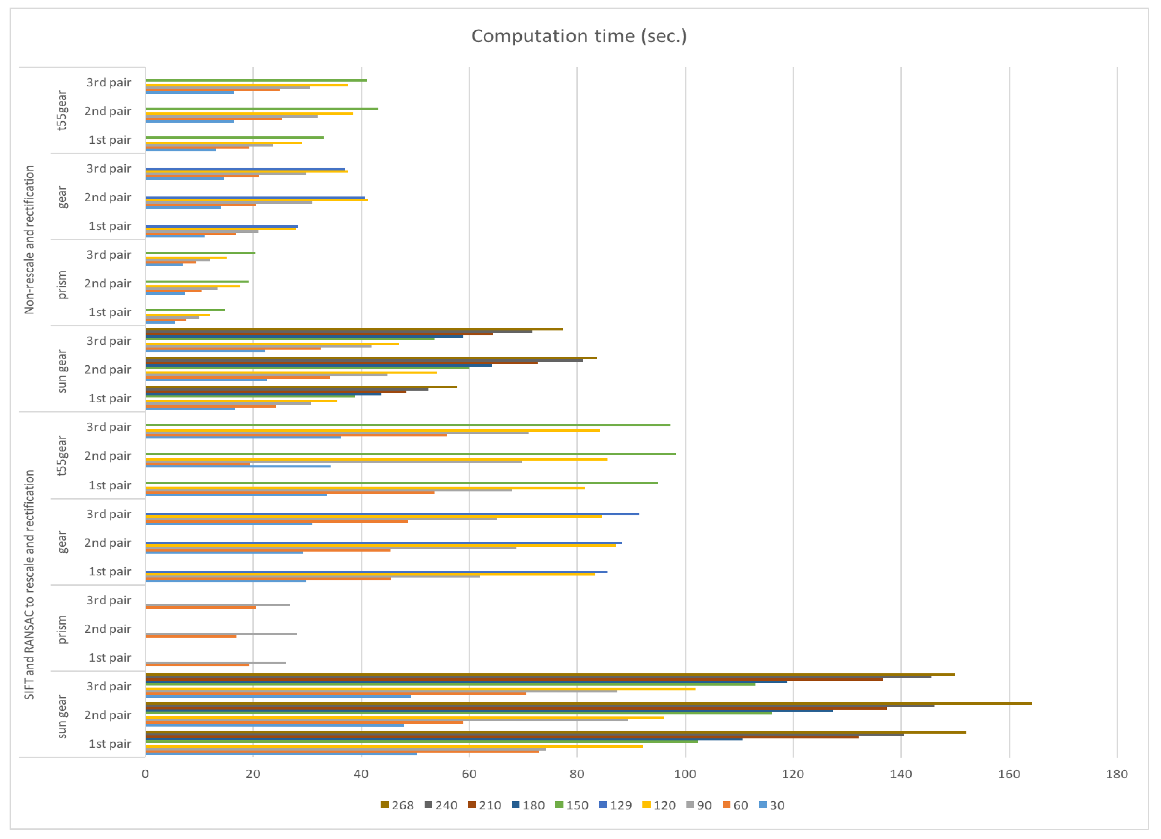
Figure 10 shows that most of the errors are greater than 10% for each geometry except the sun gear model at layers 60 to 240, where the error is less than 10%. The printing layers at 30, 120, and 150 layers in the prism model had zero error percentage because the SIFT and RANSAC did not have enough matching points to rescale. Therefore, they could not calculate 3-D object points. In sun gear, gear, and t55gear graph, there were some printing layers for which the error percentage showed a huge difference because the SIFT and RANSAC had the wrong matching and were rescaling at the wrong size. The computation time (as seen in Figure 11) depends on the size and the shape of the 3-D reconstruction. Most of the models had the same trend of the computation time, which increased when the printing layers were increasing except for the prism model because it could not reconstruct a 3-D model. The sun gear model is the largest size, so the computation time for each pair of cameras took longer than other models (i.e., (~170 s per pair). It took about 510 s to detect an error for three pairs of sun gear images.

Failure Printing State

Figure 12 shows that most of the errors are greater than 10% for each geometry except the third pair of the sun gear model after 90 layers, and the third pair of images in the gear model for all cases that the errors are less than 10%. The computation time (as seen in Figure 13) had the same trend as the normal printing state.

3.1.2. With Non-Rescale and Rectification

Normal Printing State

Figure 14 shows that the errors of all models are less than 10%. The computation time (as seen in Figure 15) depends on the size and the shape of the 3-D reconstruction. Most of the models showed the same trend of the computation time: it increased when the printing layers were increasing. The sun gear model is the largest size, so the computation time for each pair of cameras took longer than other models, and it took around 100 s for each pair. It took about 300 s to detect an error for all three pairs of sun gear images. On the other hand, the prism gear is the smallest size, so the total computation time for all three pairs of images took only 60 s to calculate the errors.

Failure Printing State

Figure 16 shows that most of the errors are greater than 10% except for some layers of the sun gear model in the third pair of the images, which are less than 10%. The computation time (as seen in Figure 17) trends are similar to the normal printing state.

3.2. Error Detection

From image pre-processing, the experiment shows that the non-rescale and rectification technique can detect an error more accurately than the SITF and RANSAC rescale and rectification methods. The error detection method needs to be improved here and tested with horizontal magnitude, and horizontal and vertical magnitude.

3.2.1. Horizontal Magnitude

The results are the same as the image pre-processing experiment for the non-rescale and rectification technique for both normal printing and failure state.

3.2.2. Horizontal and Vertical Magnitude

Normal Printing State

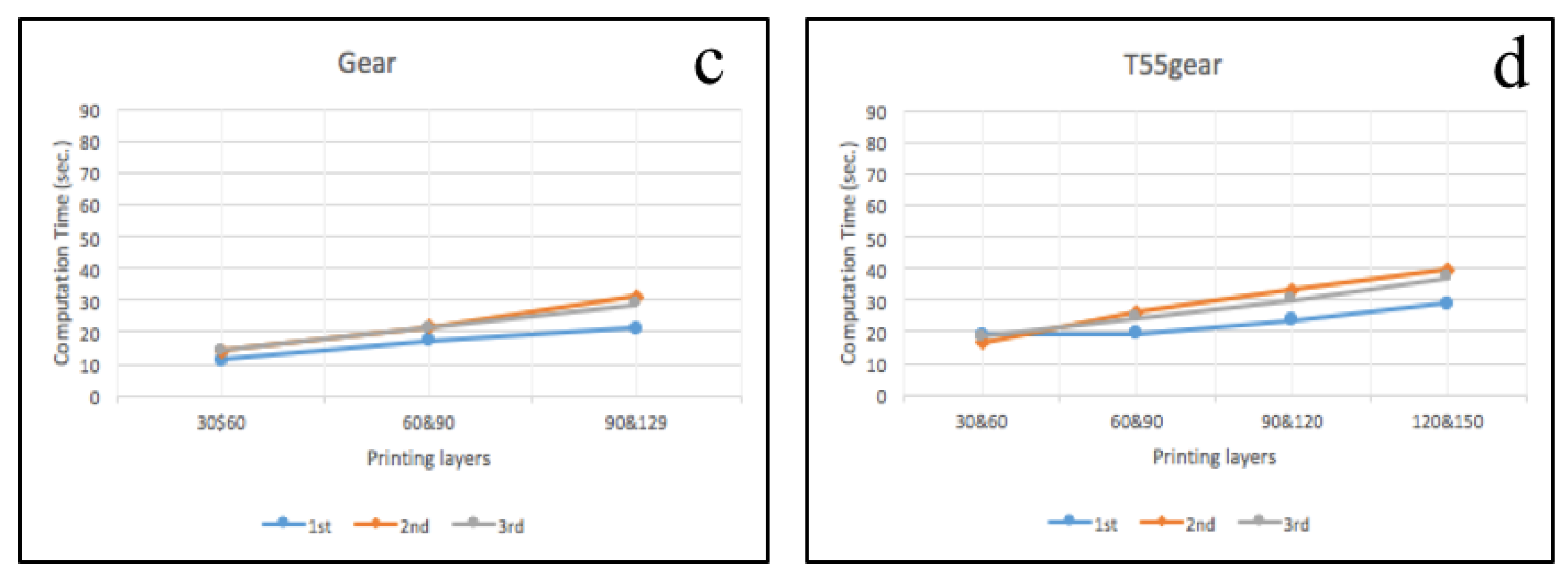
Figure 18 shows that all errors are less than 10% for each geometry. The computation time (as seen in Figure 19) depends on the size and the shape of the 3-D reconstruction. The computation time trends are similar to the horizontal magnitude method.

Failure Printing State

All cases in this section were supposed to be an error and all of them reported the errors. The computation time as shown in Figure 20 depends on the size and the shape of the 3-D reconstruction similar to the failure state of the non-rescale and rectification in the image pre-processing experiment in Figure 17.
The summary of the image pre-processing experiment for SIFT and RANSAC rescale and rectification: the non-rescale and rectification method for both normal printing and failure state are shown in Appendix A. In the normal state, the non-rescale and rectification method is better than the SIFT and RANSAC rescale and rectification method in terms of both the percentage of error and computation time. It can detect an error more accurate than the SIFT and RANSAC rescale and rectification method for all models. The computation time for both normal printing state and failure state of no rescale and rectification method is 2 times faster than the SIFT and RANSAC rescale and rectification method for all models, as shown in Appendix A.
The summary of the error detection experiment for horizontal magnitude, and horizontal and vertical magnitude for both normal printing and failure state are shown in Appendix A. In the normal printing state, both the horizontal magnitude, and the horizontal and vertical magnitudes can detect error correctly under 10% reliably. However, in the failure state, the horizontal and vertical magnitudes can detect the failure more accurately than the horizontal magnitude alone for all models. The computation times are the same in both normal printing and failure states.

4. Discussion

The experimental results show that the three double-camera set up, processed in Python can be used to automatically detect a 3-D printer error such as clogged extruder, loss of filament, or an incomplete project for a wide range of 3-D object geometries. These errors can be significant as new user RepRap printing has been shown to have a 20% failure rate [8]. Previous solutions depended on proprietary software and expensive hardware. This work has overcome the limitations [63,67] by reducing the computation time for multiple cameras and reducing the cost of software. This algorithm is a low-cost and open source code based on a double camera system for three perspectives around 360 degrees and it is the first to be used for delta systems. The computation time here for the similar area size of ROI using Python is around 2 times faster and less expensive than the code [63,67] with the same algorithm run in the Matlab environment which costs $2150 [75]. This is not that expensive for research or high-end 3-D printer applications, but represents a barrier to deployment in the low-cost prosumer printers used for distributed manufacturing, which generally cost in total $2500 or less (the RepRap used in this study was $500 in parts).
The double error detection works as designed. It should be noted that a printed 3-D object usually has a small error when compared with the 3-D model file and the real 3-D printed object. The image pre-processing with horizontal magnitude error detection experiment shows that the algorithm with non-rescale and rectification can detect when the printing has failed more accurately than the one using the SIFT and RANSAC rescale and rectification. However, the error detection using horizontal magnitude results in the sun gear model not being correct in some layers such as layers between 210 and 240, or between 240 and 268 in the first pair of cameras which are less than 10% in failure state and which should be greater than 10%. Therefore, the non-rescale and rectification algorithm was used in the error detection experiment with two different methods: horizontal magnitude, and horizontal and vertical magnitude. The horizontal and vertical magnitude method showed that the 3-D reconstruction error detection can detect 100% error when the printing has failed because the 3-D printed objects are smaller than the SCAD models because there are no data at the current height of the printing. The use of web cameras can be less expensive than other methods which result in more accurate error detection of a 3-D print such as a laser scanning or sensor [34], or scientific research cameras that cost about US $300 [63,67]. There are other methods to stop catastrophic failures. For example, there is a thrown rod alarm system for delta-style RepRaps, which alerts a user when electrical connections are broken if any of the linking rods lose connection with the end effector (hot end) [76] and Barker developed a similar thrown rod halt mod, which stops a print when electrical connections are broken if any of the linking rods are thrown [77]. This type of warning system only addresses one failure mode while the work described here stops printing for any failure mode. Others demand user oversight [56,57,58,59,60,78], while the system described here is automatic. The double cameras error detection algorithm (100% detection) can also detect the error better than vision-based error detection for 3-D printing processes when missing material flow (80% detection) [50]. However, the algorithm here still has limitations. First, slicing the stl model into every N layers cannot be done for some number layers that the user may want because Slic3r reports an error for removing a facet. For example, the t55gear model used here could not be sliced every 10 or 20 layers, which is why we tested every 30 layers here. Second, 3-D printing models that create too many shadows in the model after taking the images can also not be monitored in this way. In the removing background process, such models lose a lot of data of the bottom of the object in the image, causing a false error detection. Thus, the geometries that this process works for is limited. Finally, for users setting up the systems for themselves, web cameras must be selected with a focal length of 10 cm or longer and must be supported by the open source environment.
From the previous work [79], the images from the single camera set up can be processed to detect the shape error in low-cost 3-D printing, and the detection rate for both normal printing and failure state is 100%. The computation time of the single camera set up is fast: less than 10 s for all three cameras. Also, this work represented reconstructing 3-D images of 3-D objects from 2-D images that were successfully used to detect the size error of failure printing by six cameras. The computation time of the double camera set up depends on the size of the 3-D model. In this experiment, the average of the computation time is 45 s for each pair of cameras. Therefore, the single and double camera setup in an open source algorithm have been used together for more efficiency in reliable monitoring error of FFF-based 3-D printing in shape and size.
In addition, to overcome these limitations there are several other areas of future research. First, the slicing stl model process need to be investigated to eliminate the error for removing a facet. Second, removing the background algorithm needs to be more accurate to remove only noise. Furthermore, to increase the quality of removing the background, the new mathematical equations need to be tested for the performance of the system. Third, the computation time of this system would be improved if the 3-D reconstruction process is calculated only on the new area of the 3-D printed part. For example, the stl model is sliced every 30 layers. The first 3-D reconstruction is for layer 1 to 30, then the next 3-D reconstruction should be only for layer 31 to 60. This will reduce the area of pixels that needs to be calculated. In this study, errors associated with clogged nozzle, loss of filament, an incomplete project, or size error of 3-D printing were quantified. This work can be extended to the other printing challenges related to FFF-based 3-D printing discussed in the introduction. In particular, by focusing on the errors in the first several layers the following errors could be detected (warping, elephant foot, and bed adhesion), and these errors need to be quantified. Then, for subsequent layers, a reduced percent error threshold could be used to stop printing when distortion due to shrinking, skewed prints/shifted layers, and layer misalignment occurs. Lastly, this system may be tested with other block matching algorithms to see if another algorithm is faster and more ac-curate such as correlation coefficient, normalized correlation coefficient, cross correlation, normalized cross correlation, squared difference, or normalized squared difference [80]. Last, Franklin needs to be modified to include this algorithm in order to alert user and pause the printing when an error occurs.

5. Conclusions

This paper described an open-source low-cost reliable real-time monitoring platform for FFF-based 3-D printing based on a double cameras system for three perspectives around 360 degrees. The results showed that the algorithm using stereo calibration with detecting an error at the current height of the printing was effective at detecting a clogged nozzle, loss of filament, or an incomplete project for a wide range of 3-D object geometries. The error calculations were determined from the data in the 3-D reconstruction points at the current height of the printing. The error was reported when these errors exceeded 100%. The validity of this approach using our experiment shows that the error detection system is capable of a 100 percent detection rate for both normal printing and failure state.

Acknowledgments

This work was supported by the Michigan Tech Open Sustainability Technology Lab, the EE Department at MTU and a Royal Thai Scholarship.

Author Contributions

S.N. wrote the algorithm, performed all experiments and analyzed the results. M.R. and J.P. formulated the project and assisted on the analysis. All authors co-wrote and edited the manuscript.

Conflicts of Interest

The authors declare no conflict of interest.

Appendix A

The summary of the image pre-processing experiment for the SIFT and RANSAC rescale and rectification, and non-rescale and rectification method for both normal printing and failure state are shown in Figure A1, Figure A2, Figure A3 and Figure A4. In the normal state, the non-rescale and rectification method can detect an error more accurately than the SIFT and RANSAC rescale and rectification method for all models, as shown in Figure A1. However, both methods fail to detect the failure state, as shown in Figure A3. The computation time for both normal printing state and failure state of no rescale and rectification method is 2 times faster than the SIFT and RANSAC rescale and rectification method for all models, as shown in Figure A2 and Figure A4.
The summary of the error detection experiment for horizontal magnitude, and horizontal and vertical magnitude for both normal printing and failure state are shown in Figure A5, Figure A6, Figure A7 and Figure A8. In normal printing state, both horizontal magnitude, and horizontal and vertical magnitude can detect errors correctly under 10% as shown in Figure A5. However, in the failure state, the horizontal and vertical magnitude can detect the failure more accurately than the horizontal magnitude for all models by reporting 100% error as shown in Figure A7. Also, the computation times are the same in both normal printing and failure state as shown in Figure A6 and Figure A8.
Figure A1. Summary of image pre-processing: the error detection of normal printing state for (a) sun gear; (b) prism; (c) gear; and (d) t55gear.
Jmmp 01 00002 g021
Figure A2. Summary of image pre-processing: the computation time of normal printing state for (a) sun gear; (b) prism; (c) gear; and (d) t55gear.
Jmmp 01 00002 g022
Figure A3. Summary of image pre-processing: the error detection of failure state for (a) sun gear; (b) prism; (c) gear; and (d) t55gear.
Jmmp 01 00002 g023
Figure A4. Summary of image pre-processing: the computation time of failure state for (a) sun gear; (b) prism; (c) gear; and (d) t55gear.
Jmmp 01 00002 g024
Figure A5. Summary of error detection: the error detection of normal printing state for (a) sun gear; (b) prism; (c) gear; and (d) t55gear.
Jmmp 01 00002 g025
Figure A6. Summary of error detection: the computation time of normal printing state for (a) sun gear; (b) prism; (c) gear; and (d) t55gear.
Jmmp 01 00002 g026
Figure A7. Summary of error detection: the error detection of failure state for (a) sun gear; (b) prism; (c) gear; and (d) t55gear.
Jmmp 01 00002 g027
Figure A8. Summary of error detection: the computation time of failure state for (a) sun gear; (b) prism; (c) gear; and (d) t55gear.
Jmmp 01 00002 g028

References

  1. Wohlers, T. Wohlers Report 2016; Wohlers Associates, Inc.: Fort Collins, CO, USA, 2016. [Google Scholar]
  2. Sells, E.; Smith, Z.; Bailard, S.; Bowyer, A.; Olliver, V. RepRap: The Replicating Rapid Prototyper: Maximizing Customizability by Breeding the Means of Production. In Handbook of Research in Mass Customization and Personalization: Strategies and Concepts; Piller, F.T., Tseng, M.M., Eds.; World Scientific: Singapore, 2010; Volume 1, pp. 568–580. [Google Scholar]
  3. Jones, R.; Haufe, P.; Sells, E.; Iravani, P.; Olliver, V.; Palmer, C.; Bowyer, A. RepRap—The replicating rapid prototyper. Robotica 2011, 29, 177–191. [Google Scholar] [CrossRef]
  4. Bowyer, A. 3D Printing and Humanity’s First Imperfect Replicator. 3D Print. Addit. Manuf. 2014, 1, 4–5. [Google Scholar] [CrossRef]
  5. Gibb, A.; Abadie, S. Building Open Source Hardware: DIY Manufacturing for Hackers and Makers; Addison Wesley: Boston, MA, USA, 2014. [Google Scholar]
  6. Raymond, E. The cathedral and the bazaar. Knowl. Technol. Policy 1999, 12, 23–49. [Google Scholar] [CrossRef]
  7. Make. 3D Printer Shootout News, Reviews and More|Make: DIY Projects and Ideas for Makers [WWW Document]. 2017. Available online: http://makezine.com/tag/3d-printer-shootout/ (accessed on 11 April 2017).
  8. Wittbrodt, B.T.; Glover, A.G.; Laureto, J.; Anzalone, G.C.; Oppliger, D.; Irwin, J.L.; Pearce, J.M. Life-cycle economic analysis of distributed manufacturing with open-source 3-D printers. Mech. Tron. 2013, 23, 713–726. [Google Scholar] [CrossRef]
  9. Petersen, E.E.; Pearce, J. Emergence of Home Manufacturing in the Developed World: Return on Investment for Open-Source 3-D Printers. Technologies 2017, 5, 7. [Google Scholar] [CrossRef]
  10. Campbell, I.; Bourell, D.; Gibson, I. Additive manufacturing: Rapid prototyping comes of age. Rapid Prototyp. J. 2012, 18, 255–258. [Google Scholar] [CrossRef]
  11. Gibson, I.; Rosen, D.; Stucker, B. Additive Manufacturing Technologies: 3D Printing, Rapid Prototyping, and Direct Digital Manufacturing; Springer: Berlin, Germany, 2014. [Google Scholar]
  12. Kentzer, J.; Koch, B.; Thiim, M.; Jones, R.W.; Villumsen, E. An open source hardware-based mechatronics project: The replicating rapid 3-D printer. In Proceedings of the 4th International Conference on Mechatronics (ICOM), Kuala Lumpur, Malaysia, 17–19 May 2011; pp. 1–8. [Google Scholar] [CrossRef]
  13. Gwamuri, J.; Wittbrodt, B.T.; Anzalone, N.C.; Pearce, J.M. Reversing the trend of large scale and centralization in manufacturing: The case of distributed manufacturing of customizable 3-D-printable self-adjustable glasses. Chall. Sustain. 2014, 2, 30–40. [Google Scholar] [CrossRef]
  14. Irwin, J.L.; Oppliger, D.E.; Pearce, J.M.; Anzalone, G. Evaluation of RepRap 3D Printer Work-shops in K-12 STEM. In Proceedings of the 122nd ASEE Conference, Seattle, WA, USA, 14–17 June 2015. [Google Scholar]
  15. Gonzalez-Gomez, J.; Valero-Gomez, A.; Prieto-Moreno, A.; Abderrahim, M. A New Open Source 3D-Printable Mobile Robotic Platform for Education. In Advances in Autonomous Mini Robots; Springer: Berlin/Heidelberg, Germany, 2012; pp. 49–62. [Google Scholar]
  16. Schelly, C.; Anzalone, G.; Wijnen, B.; Pearce, J.M. Open-source 3-D printing technologies for education: Bringing additive manufacturing to the classroom. J. Vis. Lang. Comput. 2015, 28, 226–237. [Google Scholar] [CrossRef]
  17. Pearce, J.M.; Blair, C.M.; Laciak, K.J.; Andrews, R.; Nosrat, A.; Zelenika-Zovko, I. 3-D printing of open source appropriate technologies for self-directed sustainable development. J. Sustain. Dev. 2010, 3, 17–29. [Google Scholar] [CrossRef]
  18. Fox, S. After the factory [Manufacturing renewal]. Eng. Technol. 2010, 5, 51–61. [Google Scholar]
  19. Pearce, J.M. Applications of open source 3-D printing on small farms. Organ. Farming 2015, 1, 19–35. [Google Scholar] [CrossRef]
  20. Pearce, J.M. Building Research Equipment with Free, Open-Source Hardware. Science 2012, 337, 1301–1304. [Google Scholar] [CrossRef] [PubMed]
  21. Pearce, J.M. Open-Source Lab: How to Build Your Own Hardware and Reduce Research Costs; Elsevier: New York, NY, USA, 2014. [Google Scholar]
  22. Baden, T.; Chagas, A.M.; Gage, G.J.; Marzullo, T.C.; Prieto-Godino, L.L.; Euler, T. Correction: Open labware: 3-D printing your own lab equipment. PLoS Biol. 2015, 13, e1002175. [Google Scholar] [CrossRef] [PubMed]
  23. Coakley, M.; Hurt, D.E. 3D Printing in the Laboratory. J. Lab. Autom. 2016, 21, 489–495. [Google Scholar] [CrossRef] [PubMed]
  24. O’Neill, P.F.; Ben Azouz, A.; Vázquez, M.; Liu, J.; Marczak, S.; Slouka, Z.; Chang, H.C.; Diamond, D.; Brabazon, D. Advances in three-dimensional rapid prototyping of microfluidic devices for biological applications. Biomicrofluidics 2014, 8, 52112. [Google Scholar] [CrossRef] [PubMed]
  25. Pearce, J.M.; Anzalone, N.C.; Heldt, C.L. Open-Source Wax RepRap 3-D Printer for Rapid Prototyping Paper-Based Microfluidics. J. Lab. Autom. 2016, 21, 510–516. [Google Scholar] [CrossRef] [PubMed]
  26. Rimock, M. An Introduction to the Intellectual Property Law Implications of 3D Printing. Can. J. Law Technol. 2015, 13, 1–32. [Google Scholar]
  27. Laplume, A.; Anzalone, G.C.; Pearce, J.M. Open-source, self-replicating 3-D printer factory for small-business manufacturing. Int. J. Adv. Manuf. Technol. 2016, 85, 633–642. [Google Scholar] [CrossRef]
  28. Tech, R.P.G.; Ferdinand, J.-P.; Dopfer, M. Open Source Hardware Startups and Their Communities; Springer International Publishing: Cham, Switzerland, 2016; pp. 129–145. [Google Scholar] [CrossRef]
  29. Troxler, P.; van Woensel, C. How Will Society Adopt 3D Printing; T.M.C. Asser Press: Den Haag, The Netherlands, 2016; pp. 183–212. [Google Scholar] [CrossRef]
  30. Kleszczynski, S.; zur Jacobsmühlen, J.; Sehrt, J.T.; Witt, G. Error detection in laser beam melting systems by high resolution imaging. In Proceedings of the Solid Freeform Fabrication Symposium, Austin, TX, USA, 6–8 August 2012. [Google Scholar]
  31. Kleszczynski, S.; zur Jacobsmühlen, J.; Reinarz, B.; Sehrt, J.T.; Witt, G.; Merhof, D. Improving process stability of laser beam melting systems. In Proceedings of the Frauenhofer Direct Digital Manufacturing Conference, Berlin, Germany, 12–13 March 2014. [Google Scholar]
  32. Zur Jacobsmuhlen, J.; Kleszczynski, S.; Witt, G.; Merhof, D. Robustness analysis of imaging sys-tem for inspection of laser beam melting systems. In Proceedings of the 2014 IEEE Emerging Technology and Factory Automation (ETFA), Barcelona, Spain, 16–19 September 2014; pp. 1–4. [Google Scholar] [CrossRef]
  33. Concept Laser. Metal Additive Manufacturing Machines. 2016. Available online: http://www.conceptlaserinc.com/ (accessed on 10 November 2016).
  34. Faes, M.; Abbeloos, W.; Vogeler, F.; Valkenaers, H.; Coppens, K.; Goedemé, T.; Ferraris, E. Process Monitoring of Extrusion Based 3D Printing via Laser Scanning. Comput. Vis. Pattern Recognit. 2014, 6, 363–367. [Google Scholar] [CrossRef]
  35. Volpato, N.; Aguiomar Foggiatto, J.; Coradini Schwarz, D. The influence of support base on FDM accuracy in Z. Rapid Prototyp. J. 2014, 20, 182–191. [Google Scholar] [CrossRef]
  36. Wu, H.; Wang, Y.; Yu, Z. In situ monitoring of FDM machine condition via acoustic emission. Int. J. Adv. Manuf. Technol. 2016, 84, 1483–1495. [Google Scholar] [CrossRef]
  37. Atli, A.V.; Urhan, O.; Ertürk, S.; Sönmez, M. A computer vision-based fast approach to drilling tool condition monitoring. J. Eng. Manuf. 2006, 220, 1409–1415. [Google Scholar] [CrossRef]
  38. Bradley, C.; Wong, Y.S. Surface texture indicators of tool wear—A machine vision approach. Int. J. Adv. Manuf. Technol. 2001, 17, 435–443. [Google Scholar] [CrossRef]
  39. Bradski, G.; Kaehler, A. Learning OpenCV: Computer Vision with the OpenCV Library; O’Reilly Media, Inc.: Sebastopol, CA, USA, 2008. [Google Scholar]
  40. Edinbarough, I.; Balderas, R.; Bose, S. A vision and robot based on-line inspection monitoring system for electronic manufacturing. Comput. Ind. 2005, 56, 986–996. [Google Scholar] [CrossRef]
  41. Golnabi, H.; Asadpour, A. Design and application of industrial machine vision systems. Robot. Comput. Integr. Manuf. 2007, 23, 630–637. [Google Scholar] [CrossRef]
  42. Ji, S.; Zhang, X.; Zhang, L.; Wan, Y.; Yuan, J.; Zhang, L. Application of computer vision in tool condition monitoring. J. Zhejiang Univ. Technol. 2002, 30, 143–148. [Google Scholar]
  43. Kerr, D.; Pengilley, J.; Garwood, R. Assessment and visualization of machine tool wear using computer vision. Int. J. Adv. Manuf. Technol. 2006, 28, 781–791. [Google Scholar] [CrossRef]
  44. Klancnik, S.; Ficko, J.; Pahole, I. Computer Vision-Based Approach to End Mill Tool Monitoring. Int. J. Simul. Model. 2015, 14, 571–583. [Google Scholar] [CrossRef]
  45. Lanzetta, M. A new flexible high-resolution vision sensor for tool condition monitoring. J. Mater. Process. Technol. 2001, 119, 73–82. [Google Scholar] [CrossRef]
  46. Li, Y.; Li, Y.F.; Wang, Q.L.; Xu, D.; Tan, M. Measurement and defect detection of the weld bead based on online vision inspection. IEEE Trans. Instrum. Meas. 2010, 59, 1841–1849. [Google Scholar] [CrossRef]
  47. Pfeifer, T.; Wiegers, L. Reliable tool wear monitoring by optimized image and illumination control in machine vision. Measurement 2000, 28, 209–218. [Google Scholar] [CrossRef]
  48. Wang, W.H.; Hong, G.S.; Wong, Y.S.; Zhu, K.P. Sensor fusion for online tool condition monitoring in milling. Int. J. Prod. Res. 2007, 45, 5095–5116. [Google Scholar] [CrossRef]
  49. Hurd, S.; Camp, C.; White, J. Quality Assurance in Additive Manufacturing through Mobile Computing; Springer: Cham, Switzerland, 2015; pp. 203–220. [Google Scholar]
  50. Baumann, F.; Roller, D. Vision based error detection for 3D printing processes. MATEC Web Conf. 2016, 59, 06003. [Google Scholar] [CrossRef]
  51. Straub, J. Initial work on the characterization of additive manufacturing (3D printing) using soft-ware image analysis. Machines 2015, 3, 55–71. [Google Scholar] [CrossRef]
  52. OpenCV. OpenCV library 2016. Available online: http://opencv.org/ (accessed on 10 November 2016).
  53. Python. Welcome to Python.org 2016. Available online: https://www.python.org/ (accessed on 10 November 2016).
  54. Raspberry, P. Teach, Learn, and Make with Raspberry Pi 2016. Available online: https://www.raspberrypi.org/ (accessed on 3 December 2016).
  55. Microsoft. Learn to Develop with Microsoft Developer Network|MSDN 2016. Available online: https://msdn.microsoft.com/en-us/default.aspx (accessed on 13 November 2016).
  56. Gewirtz, D. Adding a Raspberry Pi case and a camera to your LulzBot Mini—Watch Video Online—Watch Latest Ultra HD 4K Videos Online 2016. Available online: http://www.zdnet.com/article/3d-printing-hands-on-adding-a-case-and-a-camera-to-the-raspberry-pi-and-lulzbot-mini/ (accessed on 30 November 2016).
  57. Printer3D. Free IP Camera Monitoring for 3D printer with old webcam usb in 5min—3D Printers English French & FAQ Wanhao Duplicator D6 Monoprice Maker Ultimate & D4, D5, Duplicator 7. 2017. Available online: http://www.printer3d.one/en/forums/topic/free-ip-camera-monitoring-for-3d-printer-with-old-webcam-usb-in-5min/ (accessed on 18 March 2017).
  58. Carmelito. Controlling and Monitoring your 3D printer with...|element14|MusicTech 2016. Available online: https://www.element14.com/community/community/design-challenges/musictech/blog/2016/03/16/controlling-your-3d-printer-with-beaglebone-and-octoprint (accessed on 18 March 2017).
  59. Simon, J. Monitoring Your 3D Prints|3D Universe 2017. Available online: https://3duniverse.org/2014/01/06/monitoring-your-3d-prints/ (accessed on 18 March 2017).
  60. Ken, V. Logitech C170 webcam mount for daVinci 3D Printer by KenVersus—Thingiverse. 2015. Available online: http://www.thingiverse.com/thing:747105 (accessed on 18 March 2017).
  61. Lowe, D.G. Object recognition from local scale-invariant features. In Proceedings of the Seventh IEEE International Conference on Computer Vision, Washington, DC, USA, 20–25 September 1999; Volume 2, pp. 1150–1157. [Google Scholar]
  62. Fischler, M.A.; Bolles, R.C. Random sample consensus: A paradigm for model fitting with applications to image analysis and automated cartography. Commun. ACM 1981, 24, 381–395. [Google Scholar] [CrossRef]
  63. Nuchitprasitchai, S.; Roggemann, M.C.; Havens, T.C. Algorithm for Reconstructing Three Dimensional Images from Overlapping Two Dimensional Intensity Measurements with Relaxed Camera Positioning Requirements to reconstruct 3D image. IJMER 2016, 6, 69–81. [Google Scholar]
  64. Anzalone, G.C.; Wijnen, B.; Pearce, J.M. Multi-material additive and subtractive prosumer digital fabrication with a free and open-source convertible delta RepRap 3-D printer. Rapid Prototyp. J. 2015, 21, 506–519. [Google Scholar] [CrossRef]
  65. Anzalone, G.; Wijnen, B.; Pearce, J.M. Delta Build Overview: MOST—Appropedia: The sustainability wiki 2016. Available online: http://www.appropedia.org/Delta_Build_Overview:MOST (accessed on 13 June 2016).
  66. Rostock. RepRapWiki 2016. Available online: http://reprap.org/wiki/Rostock (accessed on 5 November 2016).
  67. Nuchitprasitchai, S.; Roggemann, M.; Pearce, J. Factors Effecting Real Time Optical Monitoring of Fused Filament 3-D Printing. Prog. Addit. Manuf. 2017. [Google Scholar] [CrossRef]
  68. OpenCV. Camera Calibration and 3D Reconstruction—OpenCV 2.4.13.2 documentation. 2016. Available online: http://docs.opencv.org/2.4/modules/calib3d/doc/camera_calibration_and_3d_reconstruction.html#stereobm (accessed on 3 December 2016).
  69. Dollar Tree, Inc. Floral Supplies, Party Supplies, Cleaning Supplies. 2016. Available online: https://www.dollartree.com/ (accessed on 3 December 2016).
  70. Thing-O-Fun. Exploded Planetary Gear Set by Thing-O-Fun—Thingiverse. 2012. Available online: http://www.thingiverse.com/thing:18291 (accessed on 3 December 2016).
  71. Jetty. Paper Crimper by jetty—Thingiverse. 2012. Available online: http://www.thingiverse.com/thing:17634 (accessed on 3 December 2016).
  72. Droffarts. Parametric pulley—lots of tooth profiles by droftarts—Thingiverse. Available online: http://www.thingiverse.com/thing:16627 (accessed on 12 March 2017).
  73. Nuchitprasitchai, S. 3-D models. 2017. Available online: https://osf.io/utp6g/ (accessed on 5 April 2017).
  74. Wijnen, B.; Anzalone, G.C.; Haselhuhn, A.S.; Sanders, P.G.; Pearce, J.M. Free and open-source control software for 3-D motion and processing. J. Open Res. Softw. 2016, 4, e2. [Google Scholar]
  75. MathWorks. Pricing and Licensing—MATLAB & Simulink. 2016. Available online: https://www.mathworks.com/pricing-licensing.html?intendeduse=comm (accessed on 8 December 2016).
  76. Nuchitprasitchai, S. Rod alarm—Appropedia: The sustainability wiki. 2016. Available online: http://www.appropedia.org/Rod_alarm (accessed on 20 March 2017).
  77. Barker, B. Thrown Rod Halt Mod—Appropedia: The sustainability wiki. Available online: http://www.appropedia.org/Thrown_Rod_Halt_Mod (accessed on 20 March 2017).
  78. Mahan, T. Raspberry Pi Control and Wireless Interface—Appropedia: The sustainability wiki. 2016. Available online: http://www.appropedia.org/Raspberry_Pi_Control_and_Wireless_Interface (accessed on 20 March 2017).
  79. Nuchitprasitchai, S.; Roggemann, M.; Pearce, J. An Open Source Algorithm for Reconstruction 3-D images for Low-cost, Reliable Real-time Monitoring of FFF-based 3-D Printing. 2017; submitted. [Google Scholar]
  80. Abidrahmank. OpenCV2-Python-Tutorials. 2014. Available online: https://github.com/abidrahmank/OpenCV2-Python-Tutorials/ (accessed on 30 March 2017).
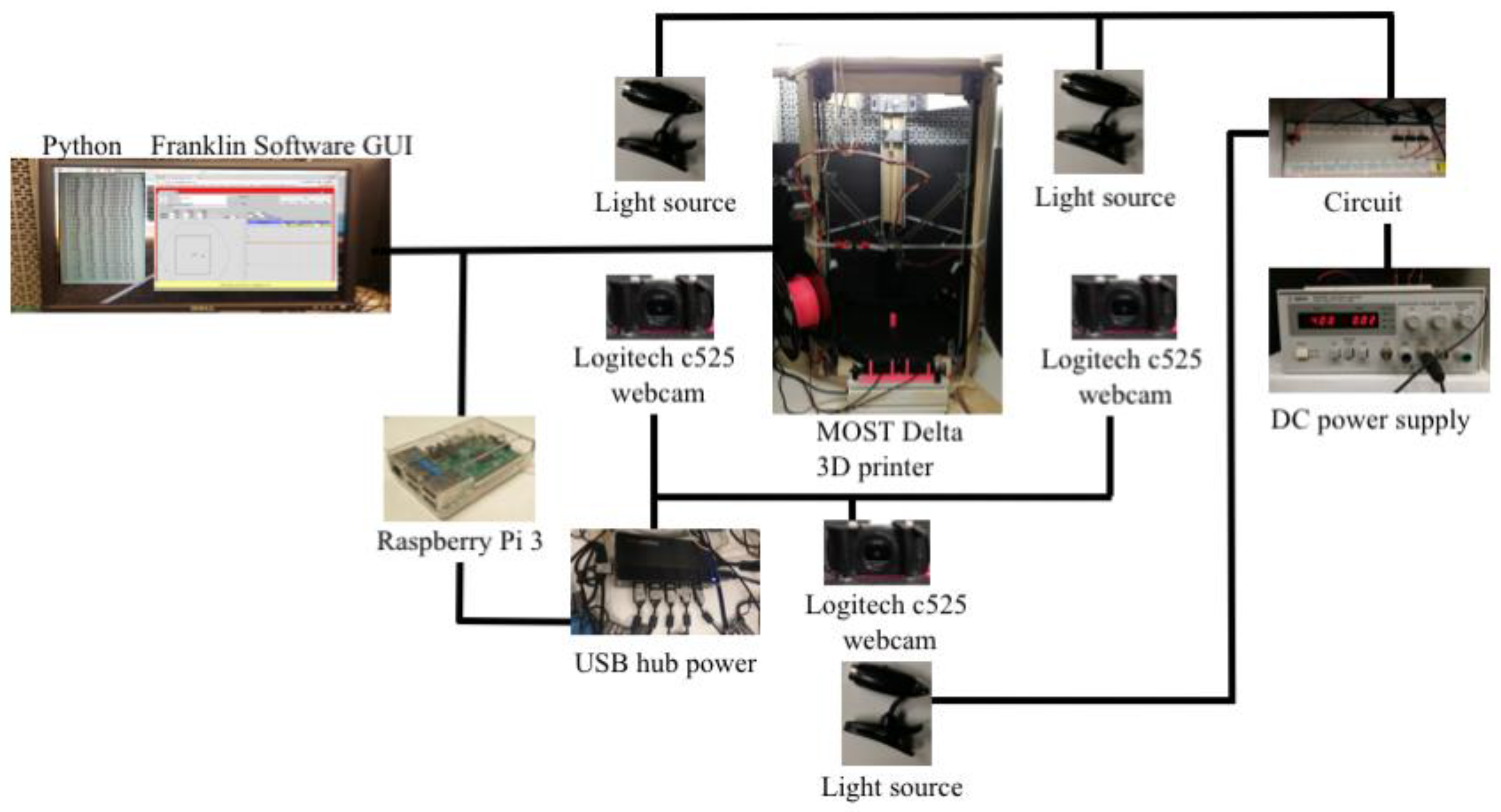
Figure 1. MOST (Michigan Tech Open Sustainability Technology) Delta printer experimental setup where three pairs of cameras were placed around the 3-D printer 120 degrees apart then all six images were processed by our Python-algorithms on Raspberry Pi3.
Jmmp 01 00002 g001
Figure 2. Example of reconstructing 2-D images to 3-D image.
Jmmp 01 00002 g002
Figure 3. Logitech C525 webcam: (a) webcam circuit board and body; and (b) sensor of webcam.
Jmmp 01 00002 g003
Figure 4. Example of the checkerboard image where the square size is 7-by-7.
Jmmp 01 00002 g004
Figure 5. Slicing stl file flowchart.
Jmmp 01 00002 g005
Figure 6. Python code for pausing and moving the extruder to take images.
Jmmp 01 00002 g006
Figure 7. Rendering of STereoLithography (STL) models for testing: (a) sun gear; (b) prism; (c) gear; and (d) t55gear.
Jmmp 01 00002 g007
Figure 8. The double camera error detection system flowchart.
Jmmp 01 00002 g008
Figure 9. The example of full model of sun gear image results from the first, the second and the third pair of cameras respectively: (ac) the images from the left camera; and (df) the images from the right camera.
Jmmp 01 00002 g009
Figure 10. Image pre-processing—SIFT and RANSAC rescale and rectification: the error detection of normal printing state for (a) sun gear; (b) prism; (c) gear; and (d) t55gear.
Jmmp 01 00002 g010
Figure 11. Image pre-processing—SIFT and RANSAC rescale and rectification: the computational time of normal printing state for (a) sun gear; (b) Prism; (c) gear; and (d) t55gear.
Jmmp 01 00002 g011
Figure 12. Image pre-processing—SIFT and RANSAC rescale and rectification: the error detection of failure state for (a) sun gear; (b) Prism; (c) gear; and (d) t55gear.
Jmmp 01 00002 g012aJmmp 01 00002 g012b
Figure 13. Image pre-processing—SIFT and RANSAC rescale and rectification: the computational time of failure state for (a) sun gear; (b) Prism; (c) gear; and (d) t55gear.
Jmmp 01 00002 g013
Figure 14. Image pre-processing—Non-rescale and rectification: the error detection of normal printing state for (a) sun gear; (b) Prism; (c) gear; and (d) t55gear.
Jmmp 01 00002 g014
Figure 15. Image pre-processing—Non-rescale and rectification: the computation time of normal printing state for (a) sun gear; (b) prism; (c) gear; and (d) t55gear.
Jmmp 01 00002 g015
Figure 16. Image pre-processing—Non-rescale and rectification: the error detection of failure state for (a) sun gear; (b) prism; (c) gear; and (d) t55gear.
Jmmp 01 00002 g016
Figure 17. Image pre-processing—Non-rescale and rectification: the computation time of failure state for (a) sun gear; (b) prism; (c) gear; and (d) t55gear.
Jmmp 01 00002 g017
Figure 18. Error detection—Horizontal magnitude: the error detection of normal printing state for (a) sun gear; (b) Prism; (c) gear; and (d) t55gear.
Jmmp 01 00002 g018
Figure 19. Error detection—Horizontal magnitude: the computation time of normal printing state for (a) sun gear; (b) Prism; (c) gear; and (d) t55gear.
Jmmp 01 00002 g019
Figure 20. Error detection—Horizontal and vertical magnitude: the computation time of failure state for (a) sun gear; (b) Prism; (c) gear; and (d) t55gear.
Jmmp 01 00002 g020aJmmp 01 00002 g020b