A Unique Methodology for Tool Life Prediction in Machining

Abstract

In this paper, a unique approach for estimating tool life using a hybrid finite element method coupled with empirical wear rate equation is presented. In the proposed approach, the computational time was significantly reduced when compared to nodal movement technique. However, to adopt such an approach, the angle between tool’s rake and flank faces must be constant through the process and at least two cutting experiments need to be performed for empirical model calibration. It is also important to predict the sliding velocity along the tool/flank face interface accurately when using Usui’s model to predict the tool wear rate. Model validations showed that when the sliding velocity was assumed to be equivalent to the cutting speed, poor agreement between the predicted and measured wear rate and tool life was observed, especially at low cutting speed. Furthermore, a new empirical model to predict tool wear rate in the initial or break-in period as a function of Von Mises stress field was developed. Experimental validation shows that the newly developed model substantially improved the initial tool wear rate in terms of trend and magnitude.

1. Introduction

In machining, the tool is gradually worn and loses its effective geometry. The wear is usually due to the severe thermal and mechanical loading conditions along the contacting interfaces. As wear reaches to a critical size, the tool is reached to the end of its efficient life and must be replaced. Otherwise, it affects the dimensional accuracy and surface integrity of the machined component.

Traditionally there have been two main approaches used to predict tool life: In the first approach, empirical equations were developed based on the relations between tool life and process parameters such as cutting speed, feed rate, and depth of cut. One of the most famous examples is the Taylor’s tool life equation [1], as shown in Equation (1). Although the Taylor equation is easy to use, its calibrations require extensive amount of tool life tests and data fitting [2]. Also the operating boundaries of the Taylor equation is very narrow and recalibration is usually required when the cutting tool geometry changes. In the second approach, tool wear rate has been described based on the wear mechanisms in the cutting zone. In this approach, rate of tool wear has been related to the thermomechanical process variables as shown in Equation (2). These relationships were proposed by Shaw and Dirke [3] and Trigger and Chao [4]. Following them, other researchers have developed more or less similar relations. Among them the equation proposed by Usui [5], as shown in Equation (2), is one of the most commonly used.

Taylor’s Model [1]

$$\mathrm{T}{\mathrm{V}}^{1/\mathrm{n}}{\mathrm{f}}^{1/\mathrm{m}}{\mathrm{b}}^{1/l}=\mathrm{C}$$

(1)

where, T = tool life (s), V = cutting speed (m/s), f = chip thickness (m), b = depth of cut (m), n, m, l, C = equation constants which depend on the combination of work and tool materials and cutting conditions.

Usui’s model [5]

$$\mathrm{dW}/\mathrm{dt}={\mathrm{B}}_1{\mathsf{\sigma }}_{\mathrm{n}}{\mathrm{v}}_{\mathrm{s}}{\mathrm{e}}^{(-{\mathrm{B}}_2/\mathrm{T})}$$

(2)

where, $\mathrm{dW}/\mathrm{dt}$, total wear rate (µm/s); vs, sliding velocity of the work material (m/s); ${\mathsf{\sigma }}_{\mathrm{n}}$, normal pressure on the tool face (Pa); T, temperature on the tool face (°C); B₁, B₂, equation constants which depend on the combination of work and tool materials and cutting conditions.

Usui’s equation was developed based on the principles of Shaw’s equation [3] for adhesive wear and introduction of the thermal softening factor. The total wear rate was related to the interface temperature, contact pressure, and sliding velocity of the chip or work material passing over the tool rake or flank faces respectively. Kitagawa et al. [6,7] showed that flank and crater wear on carbide tools can be predicted by Usui equation when cutting carbon steels with 0.15–0.46% C.

With the improvements in computational capabilities over the past decade, finite element method (FEM) has been used as a modelling technique for simulating the cutting process and estimating the temperature and stress distributions along the contacting interfaces that were difficult to measure or formulate based on either experimental or analytical techniques [8,9].

Combining the advantages of FEM and wear rate equations, researchers have attempted to develop physics-based methodologies for two dimensional [10,11,12,13] and three-dimensional tool wear predictions [14,15]. In all these wear prediction attempts, the cutting process with defined tool edge geometry was simulated with FEM until the mechanical and thermal loadings on the cutting tool reached steady state. Depending on the wear rate equation the required variables on interfacial nodes such as temperature, contact pressure, and sliding velocity were determined from the simulation. Following on from here, the wear rate at each node and the interfacial nodal displacements were calculated at a specified time increment. Finally, the tool geometry was updated, and the length of flank wear, VB, or depth of crater, KT, was determined. If the tool wear criterion has not been reached, the updated tool geometry was inserted back in the cutting simulation and same cycle was continued until the wear criterion was achieved. The flow chart of this methodology is shown in Figure 1. Regardless of the wear prediction accuracy, two key factors have been identified: The first referred to the nodal wear rate and displacement calculation. Calculating the displacement rate of each node along the tool–workpiece interface highly relies on the state of contact simulation, which is very complex in metal cutting. The complexity generally resulted in uncertainties in the simulated process variables such as sliding velocity which could lead to errors in nodal displacement calculation and consequently irregularity on updated worn geometry [16]. To overcome this issue, Malakizadi et al. [17] and Hosseinkhani and Ng [18] developed methodologies to determine the rate of tool material loss on the flank face from average values of interface temperature and contact pressure instead of calculating the individual nodal displacement rates.

The other factor refers to the iterative nature of tool wear prediction procedure which makes the overall computational time long and expensive. When using the approach detailed in Figure 1, a simulated cutting time increment should be defined based on which nodal displacements are calculated and cutting edge geometry is updated. Generally, the magnitude of simulated cutting time increment with respect to the total cutting time specifies the number of iterations required until the wear criterion is reached. Based on the selected time increment, Filice et al. [12], Attanasio et al. [14], and Malakizadi et al. [17] went through 10, 16, and 8 iterations, respectively. The iterative approach of Figure 1 is referred to as the series since the start of each iteration depends on the completeness of the previous iteration.

In the present paper, a new methodology for tool life prediction has been proposed and its feasibility has been investigated. This unique approach adopts the parallel processing rather than the series, which will substantially reduce the computational time. However, to adopt this approach, the angle between the tool rake and flank faces cannot vary with the increase in the flank wear length. Tool life experimental tests were carried out to identify the operating limits of such approach and validate the predicted tool life. A medium carbon steel was used in this research and orthogonal cutting was performed with an uncoated carbide tool. The motivation behind proposing this methodology was to improve the hybrid finite element/empirical based tool life prediction in terms of the wear rate calculation approach and overall computational time, which were introduced as challenges in the previous paragraphs.

2. Experimental Work

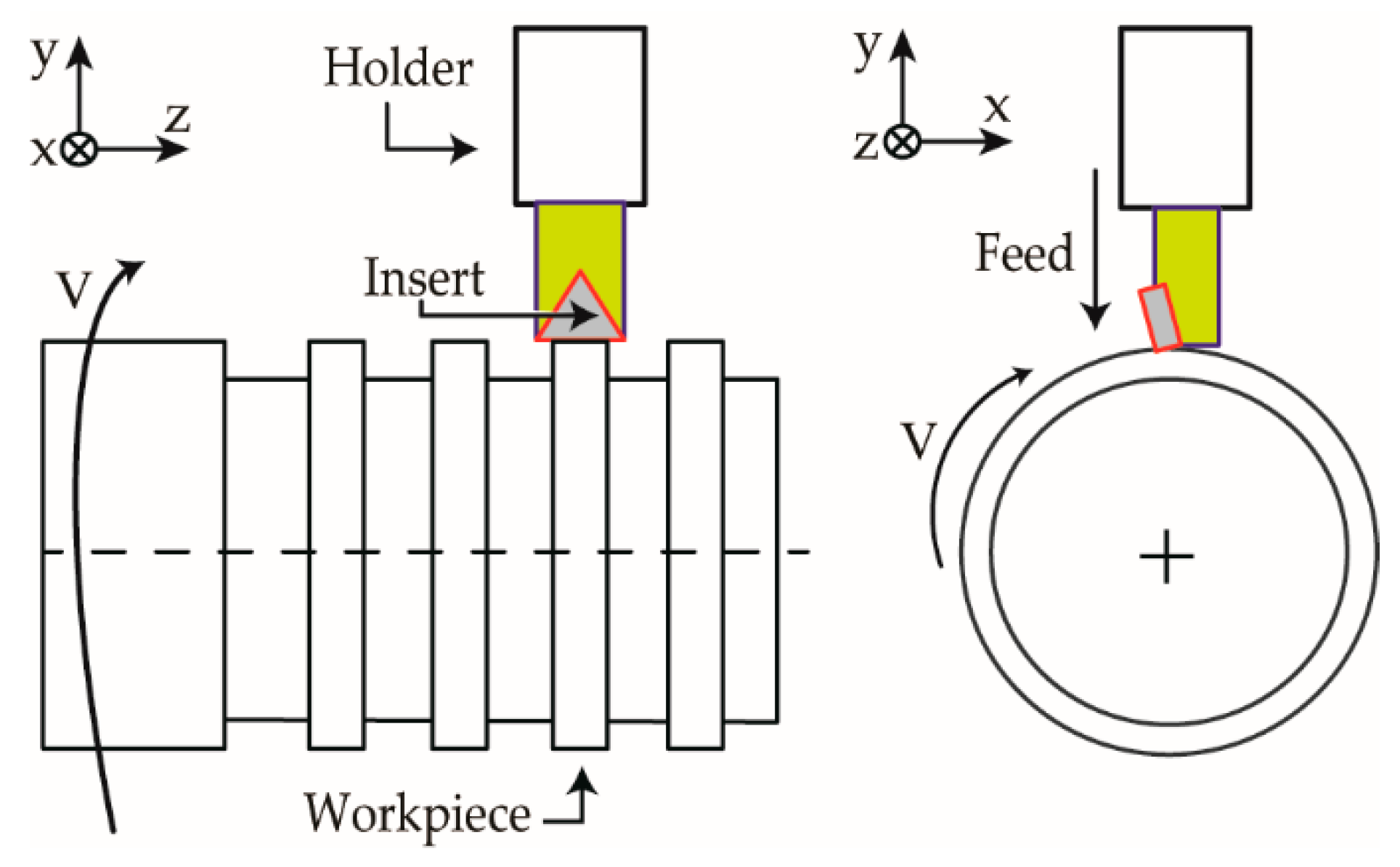
Cutting experiments were performed based on the orthogonal cutting configuration as shown in Figure 2. The ranges of cutting parameters used in this research have been listed in

Table 1. Cutting parameters.

Cutting Speed (m/min)	200 to 300
Feed Rate (mm/rev)	0.15 to 0.25
Depth of Cut (mm)	3
Rake Angle (°)	−6

. Cutting tool was uncoated tungsten carbide, with TNMG332QM-H13A designation, and work material was fully annealed AISI 1045 with hardness of 165–190 BHN. Depth of cut and rake angle were held constant at 3 mm and −6° respectively.

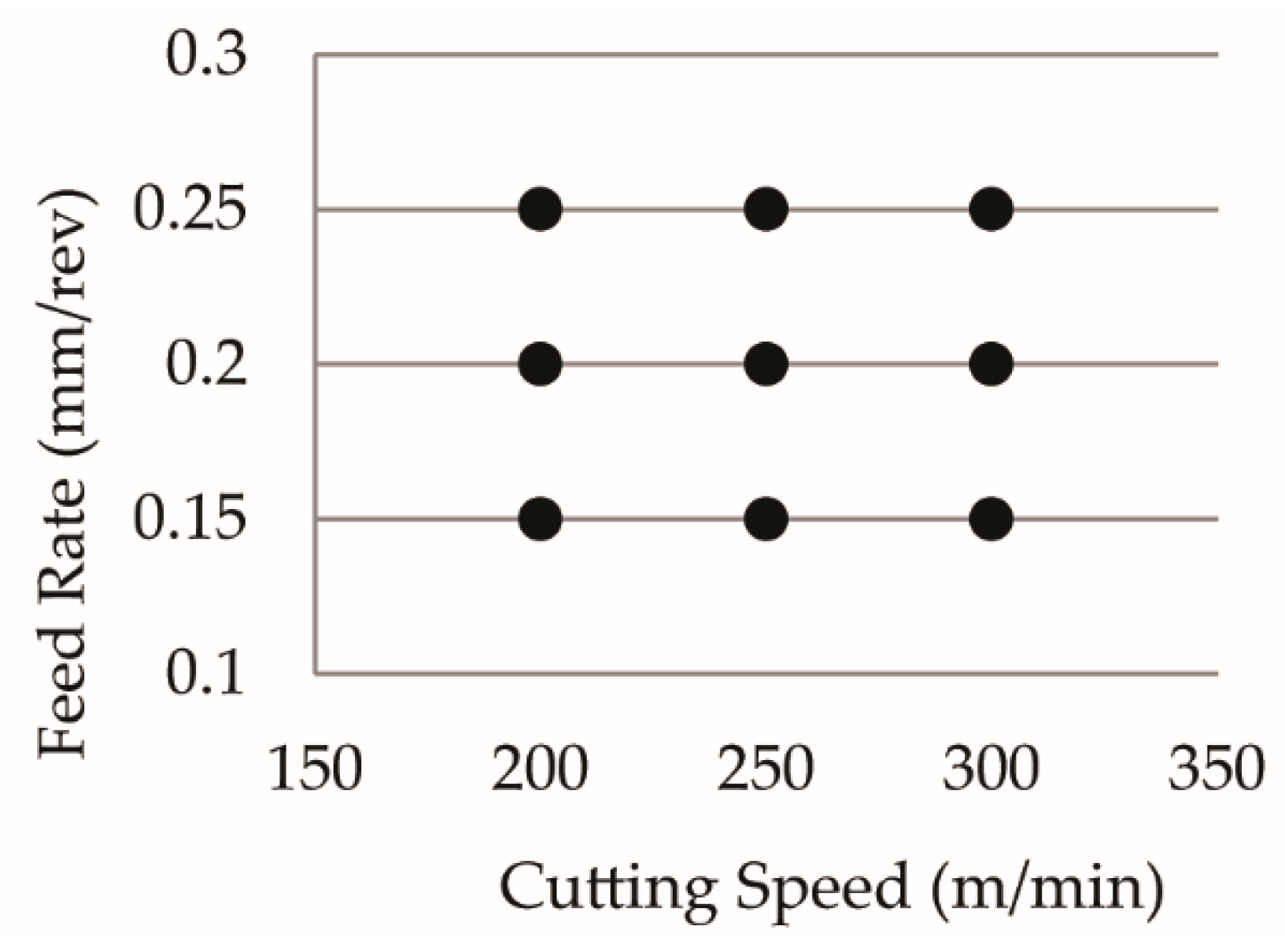
Figure 3 shows nine combinations of cutting speed and feed rate. For each combination of parameters, tool life test was performed twice and worn tool geometries were analyzed during the tests. Each test was repeated twice. Flank wear of 0.3 mm was considered as the tool life criterion for ending each tool life test which was in accordance to ISO Standard 3685 for the tool life criterion.

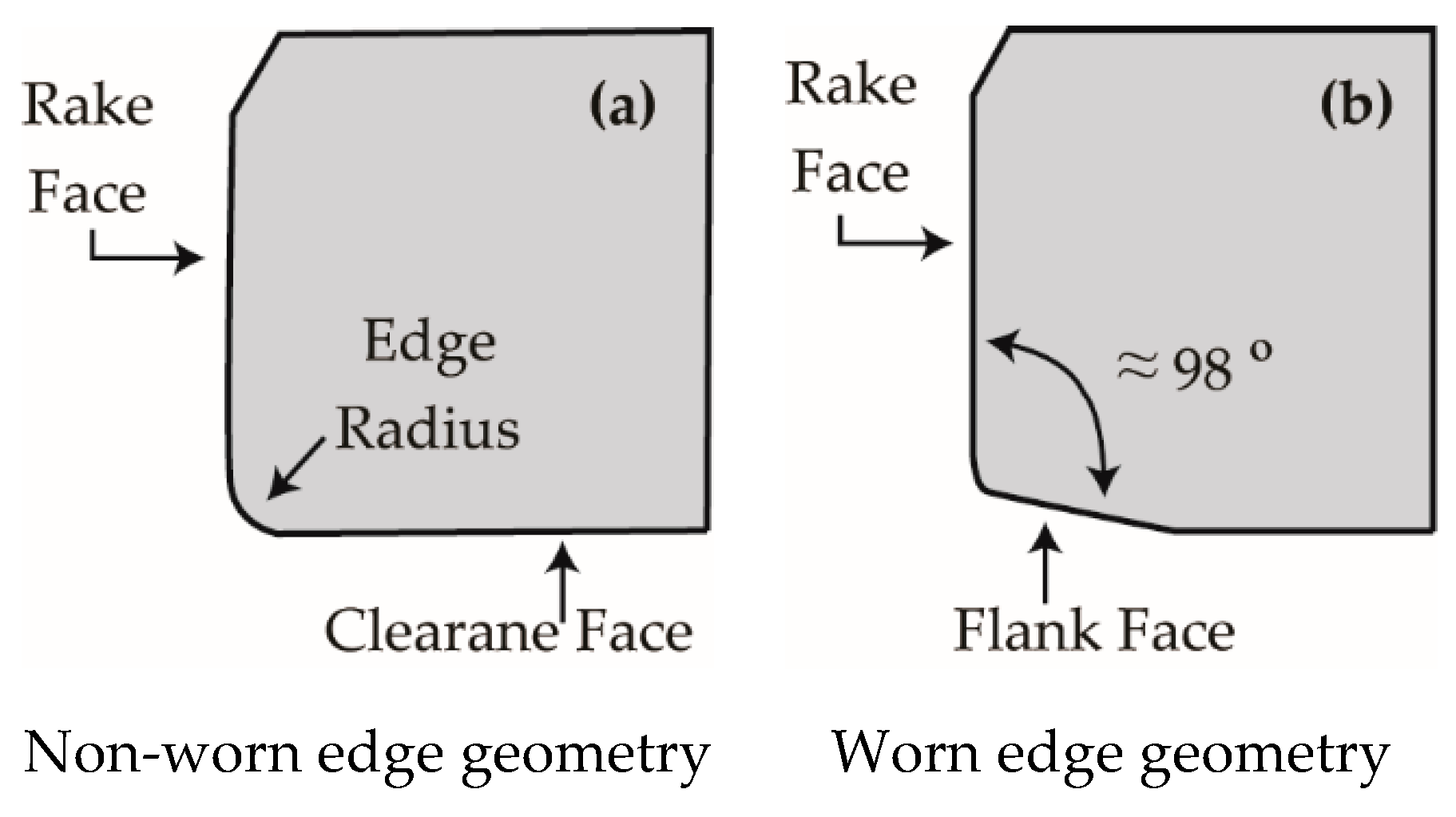
During the tool wear pattern cutting tests, after each fin was removed, the process was stopped, and tool edges were sectioned using wire electric discharge machining. The sectioned tools were then cold mounted, polished, etched, and analyzed under the optical microscope. It was observed that regardless of cutting speed and feed rate, the angle between flank and rake faces were approximately 98° at different flank wear sizes. The schematics of non-worn and worn edge geometries are shown in Figure 4. It was concluded that when cutting speed and feed rate were varied only the rate of tool wear was varied. Figure 5a–c shows the micro-graphs of tool edge geometries after machining the first fin, and Figure 5d–f shows the tool edge micro-graphs after machining the last fin with the lowest, mid-range, and highest process parameters, respectively. Lane [19] also observed similar phenomenon when machining AISI 1215 with diamond tools.

3. Tool Life Prediction Approach

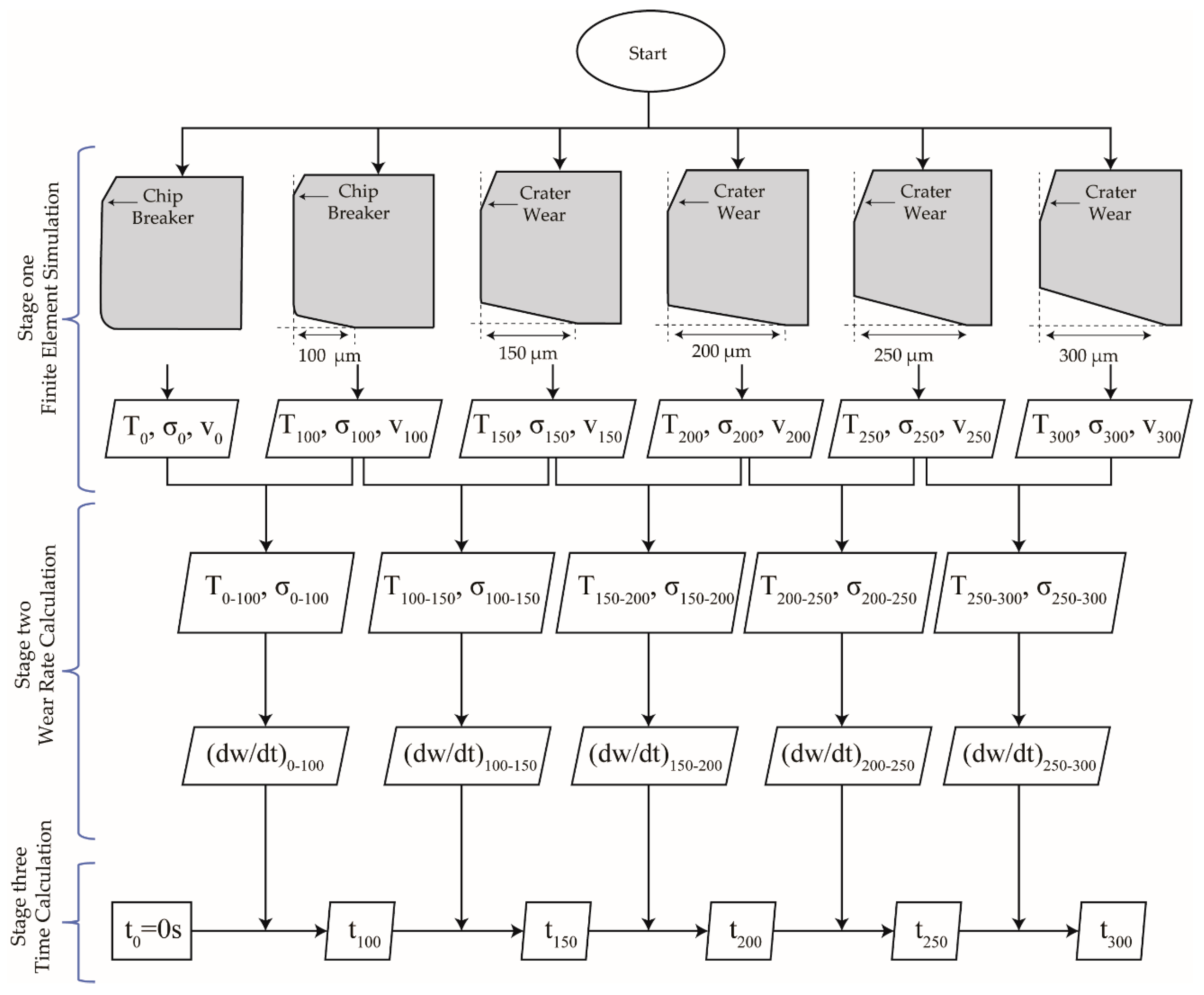
Figure 6 details the overall procedure of the current approach which has been divided into three stages. In stage one, finite element simulation is used to model the effect of flank wear length on the temperature and contact pressure at the tool flank face and workpiece interface. Six simulations are carried out in parallel for each unique set of process parameters. Each simulation will have a particular flank wear length dimension. In the current research, flank wear lengths simulated were 0, 100, 150, 200, 250, and 300 µm. In stage two, the tool life period is divided into five intervals: 0–100 µm, 100–150 µm, 150–200 µm, 200–250 µm, and 250–300 µm. The tool wear rate for each interval is calculated based on Usui’s wear rate equation together with the interface temperature and contact pressure results predicted by finite element simulation. Finally, in stage three, the tool life is calculated.

3.1. Finite Element Simulation

In stage one, FE models were built based on the principles of Arbitrary Lagrangian–Eulerian (ALE) technique. Figure 7a shows the schematic of an ALE cutting model with the associated boundary conditions. Details of the ALE technique in modeling the cutting process with non-worn and worn tool edge geometries can be found in [20]. Explicit solver in Abaqus was used with adaptive meshing. The plane strain CPE4RT elements were used for meshing the workpiece and tool which were quadrilateral with thermal-mechanical properties. The Johnson–Cook (J–C) constitutive model was used to include the effect of strain, strain rate, and temperature on the plastic deformation of the workpiece material. The interaction between the contacting surfaces has been modeled based on the Coulomb friction law in which the sticking and sliding conditions are the functions of normal and shear stresses. Figure 7b shows the resulting chip formation simulation and the location where the temperature and contact pressure were extracted for the analysis.

For any combination of cutting speed and feed rate, simulations based on the defined edge geometries were performed in parallel until mechanical-thermal fields reached steady states at the tool–workpiece interface. Parallel simulations completely eliminate the need for defining the time increment and the gradual tool geometry update, which reduced the overall computation time significantly when compared to the series approach. Based on the defined simulated cutting time increment, Filice et al. [12] and Attanasio et al. [14] had to go through the iterations 10 and 16 times, respectively. An iteration is defined here as restarting the cutting simulation with updated cutting edge geometry. Based on the approach proposed in the current research, only six simulations were performed in parallel without any iteration. Therefore, the overall tool life prediction process based on the current parallel simulation approach only requires a few hours when compared to series approach which requires at least 48 h per iteration.

Usui’s wear rate model is a function of interface temperature, contact pressure and sliding velocity. The temperature and pressure on the flank face were stable when simulation reached steady state. However, instability was observed in the simulated sliding velocity. This is likely due to the numerical errors associated with the continuous re-mapping of the workpiece elements throughout the simulation. Therefore, cutting speed was used in the wear rate calculations instead of sliding velocity. Malakizadi [16] also made similar observation regarding the instability and used cutting speed instead of sliding velocity.

From each simulation, the temperature and contact pressure on the tool flank face were extracted. Figure 7b indicated where the temperature and contact pressure were extracted from the models. Details on the simulated results have been reported in [21]. From the simulated results, flank face temperature and contact pressure increased as the flank wear increased. Flank face temperature was also a direct function of cutting speed and feed rate with more sensitivity to cutting speed. Contact pressure on the other hand, was only sensitive to the cutting speed and did not show substantial sensitivity to the variation in feed rate.

3.2. Wear Rate Calculation

In stage two, the average values of the interface temperature and contact pressure along the tool flank face were calculated with respect to the flank wear intervals of 0–100 µm, 100–150 µm, 150–200 µm, 200–250 µm, and 250–300 µm. The procedure for calculating average interface temperature and contact pressure in each interval has been shown in

Table 2. Procedure to calculate the average process variables.

Flank Wear Intervals	Average Temperature and Pressure
0–100	${\mathrm{T}}_{0–100}=\frac{{\mathrm{T}}_0+{\mathrm{T}}_{100}}{2},\hspace{0.17em}{\mathsf{\sigma }}_{0–100}=\frac{{\mathsf{\sigma }}_0+{\mathsf{\sigma }}_{100}}{2}$
100–150	${\mathrm{T}}_{100–150}=\frac{{\mathrm{T}}_{100}+{\mathrm{T}}_{150}}{2},\hspace{0.17em}{\mathsf{\sigma }}_{100–150}=\frac{{\mathsf{\sigma }}_{100}+{\mathsf{\sigma }}_{150}}{2}$
150–200	${\mathrm{T}}_{150–200}=\frac{{\mathrm{T}}_{150}+{\mathrm{T}}_{200}}{2},\hspace{0.17em}{\mathsf{\sigma }}_{150–200}=\frac{{\mathsf{\sigma }}_{150}+{\mathsf{\sigma }}_{200}}{2}$
200–250	${\mathrm{T}}_{200–250}=\frac{{\mathrm{T}}_{200}+{\mathrm{T}}_{250}}{2},{\mathsf{\sigma }}_{200–250}=\frac{{\mathsf{\sigma }}_{200}+{\mathsf{\sigma }}_{250}}{2}$
250–300	${\mathrm{T}}_{250–300}=\frac{{\mathrm{T}}_{250}+{\mathrm{T}}_{300}}{2},{\mathsf{\sigma }}_{250–300}=\frac{{\mathsf{\sigma }}_{250}+{\mathsf{\sigma }}_{300}}{2}$

.

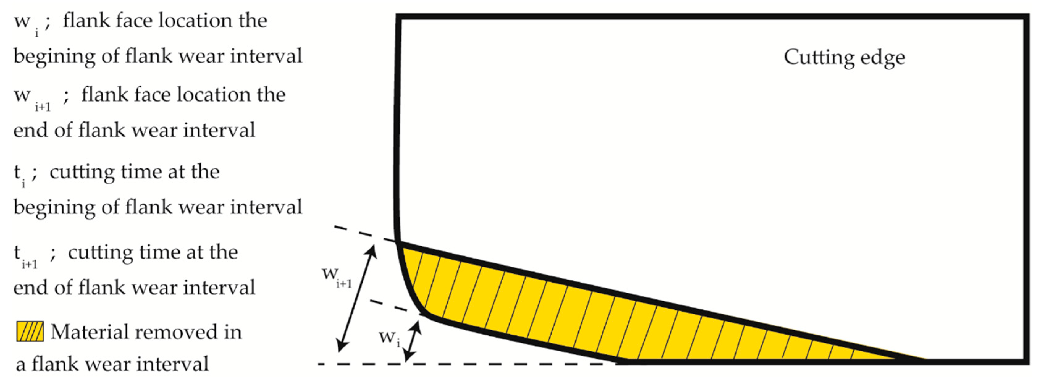
The calculated wear rate in each interval, dW/dt, represented the ratio of the distance between flank faces at the beginning, and end of that interval, Δw, to the time corresponding to that interval, Δt, as shown in Figure 8.

3.3. Cutting Time Calculation

In stage three, the cutting times corresponding to the flank wear length intervals are determined. The calculated wear rate in each interval is shown in Equation (3):

$$\mathrm{dW}/\mathrm{dt}={(\mathrm{W}}_{\mathrm{i}+1}-{\mathrm{W}}_{\mathrm{i}})/({\mathrm{t}}_{\mathrm{i}+1}-{\mathrm{t}}_{\mathrm{i}})$$

(3)

where W_i+1 and W_i are known from defined cutting edge geometries and t_i is known from the calculation of the previous interval. Equation (4) was used to estimate t_i+1.

$${\mathrm{t}}_{\mathrm{i}+1}=[({\mathrm{W}}_{\mathrm{i}+1}-{\mathrm{W}}_{\mathrm{i}})/(\mathrm{dW}/\mathrm{dt})]+{\mathrm{t}}_{\mathrm{i}}$$

(4)

This procedure was continued until the cutting time corresponding to 0.3 mm flank wear was reached, which was accordance to the ISO Standard 3685 for the tool life criterion.

4. Wear Rate Model Calibration

A general tool life trend consists of three periods which are (a) the initial or running-in period, (b) the secondary or steady-state period, and (c) the tertiary period [22]. Based on the collected experimental data in the current research, the high wear rate in the beginning of the cut differentiated the initial period from the secondary and tertiary periods. However, no extreme transition in the wear rate between secondary and tertiary periods was observed in all the nine cutting conditions carried out in this research. Therefore, the wear rate equation was calibrated in two periods. First, it was calibrated for the initial cutting period, 0–100 µm flank wear interval, and then it was calibrated for the combined second and third periods, which consisted of 100–150 µm, 150–200 µm, 200–250 µm, and 250–300 µm flank wear intervals.

The calibration in each period was performed according to a hybrid experimental/simulation approach and based on the data from two cutting conditions; V = 200 m/min – f = 0.15 mm/rev and V = 300 m/min and f = 0.25 mm/rev [21]. The constants for the calibrated equation are detailed in

Table 3. Calibrated constants of the wear rate model.

Period	B1 (m2/MN)	B2 (°C)
Initial Period	1.89 × 10−6	7141
Secondary/Tertiary Periods	1.95× 10−8	3266

. It was observed from experiments that the flank face surface orientation with respect to the rake face remained unchanged throughout the cut and tool material was continuously removed from the same direction. Therefore, in the present research, the calculation of nodal displacement rate was replaced by calculating the flank face displacement rate. Calculating the displacement rate of each node along the interface highly relies on the state of contact simulation, which is very challenging and unstable in metal cutting. In case of calculating the displacement rate of flank face, average values of temperature and contact pressure which represented all the nodal values on the interface were used. Therefore, the possibility of including the uncertainties involved in estimating the nodal displacement was eliminated.

5. Results and Discussions

5.1. Tool Life

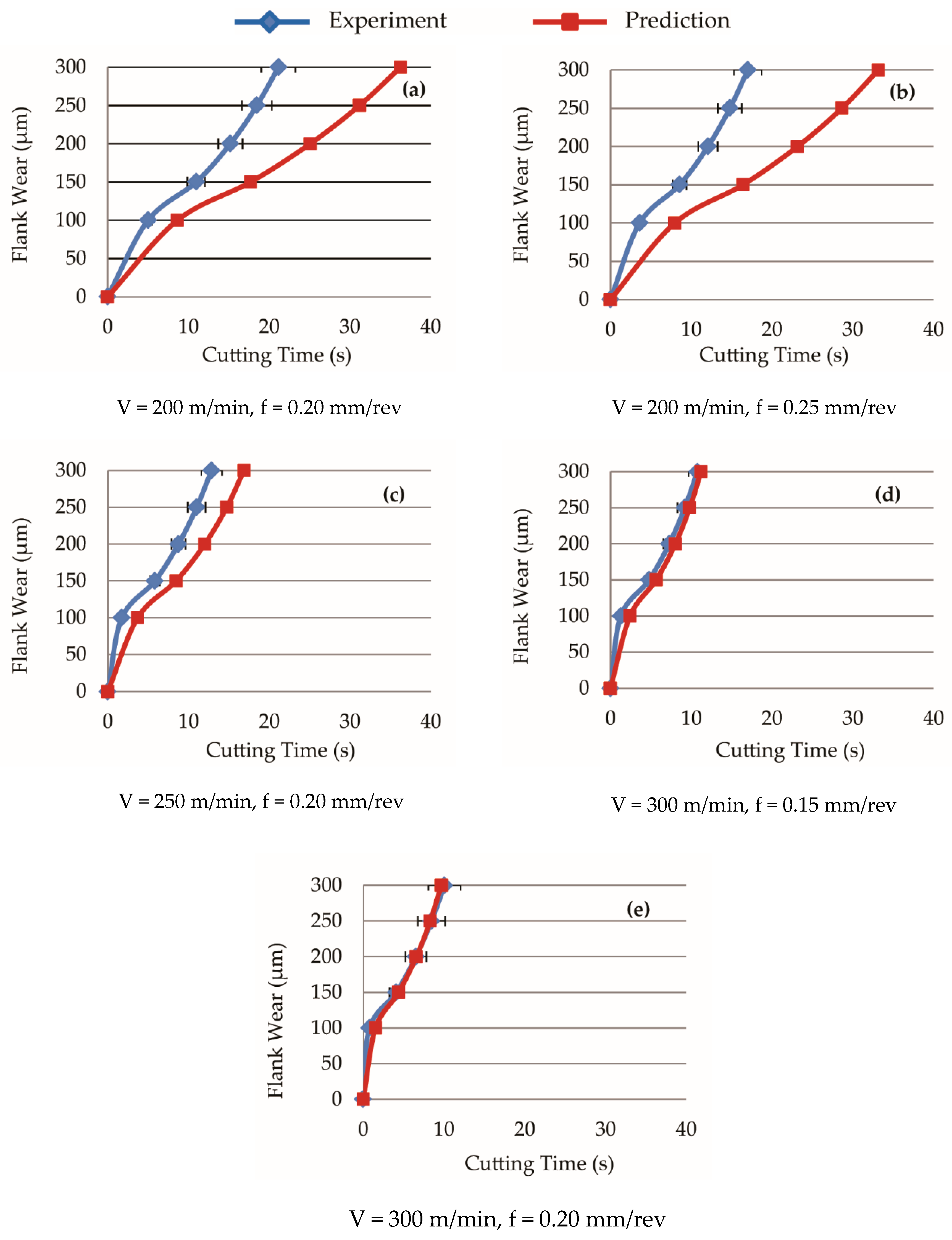
Figure 9 shows the effect of cutting speed and feed rate on the experimental and predicted tool life. In Figure 9, both experimental and predicted tool life decreased at higher cutting speed and feed rate. Binder et al. [23] and Palmai [24] made similar observations when machining AISI 1045 with carbide tools. However, in terms of tool life magnitude, the difference between predicted tool life and experiment was larger at lower cutting speeds. As shown in Figure 9a,b, at cutting speed of 200 m/min together with 0.2 mm/rev and 0.25 mm/rev feed rate, the predicted tool life were 80% and 85% longer, respectively, when compared to experiment. The difference between prediction and experiment was 30% when cutting speed was held at 250 m/min and was 10% when cutting speed was at 300 m/min regardless of feed rate, as shown in Figure 9c–e.

5.2. Wear Rate Predictions in the Initial Cutting Period

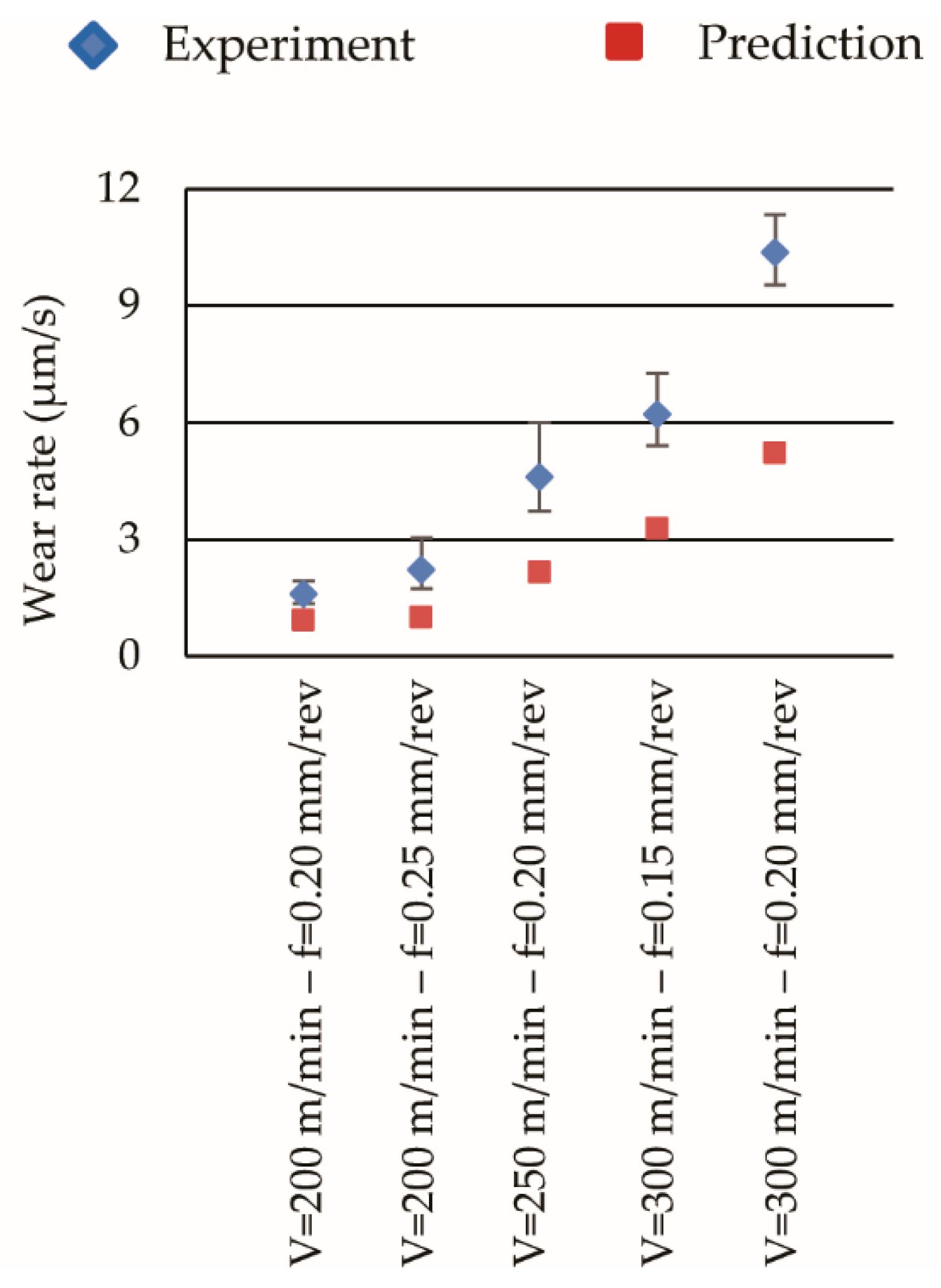
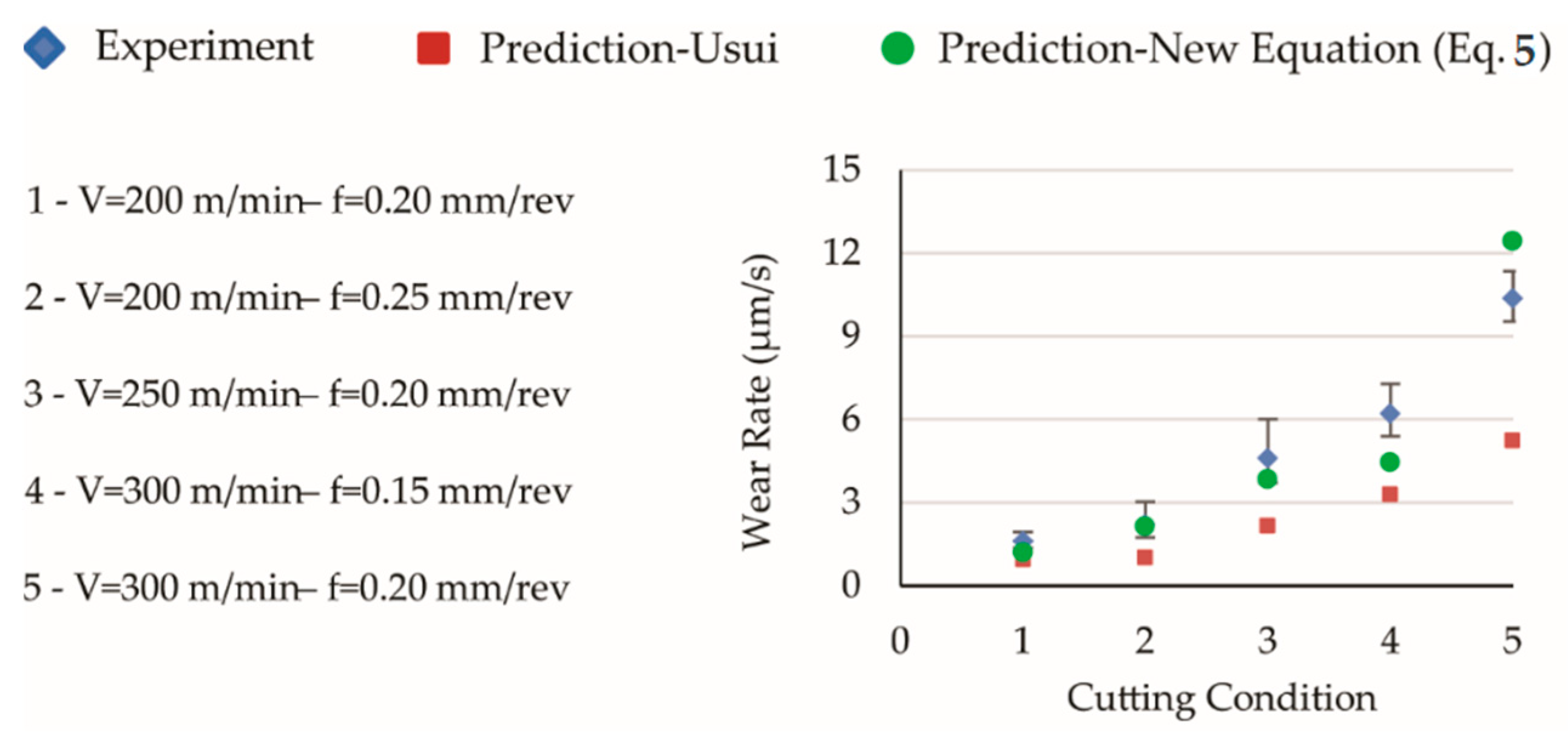
The predicted wear rates in the initial cutting periods for five cutting conditions are shown in Figure 10. The flank wear interval during the initial cutting period was between 0 and 100 µm. The predicted wear rates increased with higher cutting speed and feed rate which were similar to those observed in experiment. However, the magnitudes of predictions were not in good agreement with experiment. In the five cutting conditions analyzed, the predicted wear rates were 40% to 55% lower when compared to experiment.

The difference in the wear rate prediction in the initial period did not influence the predicted tool life in conditions with 250 m/min and 300 m/min speeds as much as it did in conditions with 200 m/min speed. This was likely due to the fact that the cutting times corresponding to the initial period were shorter in conditions with 250 m/min and 300 m/min speeds, which reduced the difference of wear rate predictions on the overall tool life.

The difference of the predictions in initial period, as shown in Figure 10, did not necessarily relate to the methodology proposed in the current research but rather due to the limitations of Usui’s model. Yen [10] referred to Usui model as an expression developed based on the principles of adhesive wear which might be better representing the flank wear rate at higher temperature and unable to capture the high initial wear rates due to micro-chipping or fracture.

5.3. Recommendation for Improvement in Wear Rate Estimation During Initial Period

The importance of successful estimation of wear rate in initial period cannot be neglected due to its influence on the overall tool life estimation, as shown in Figure 9a,b.

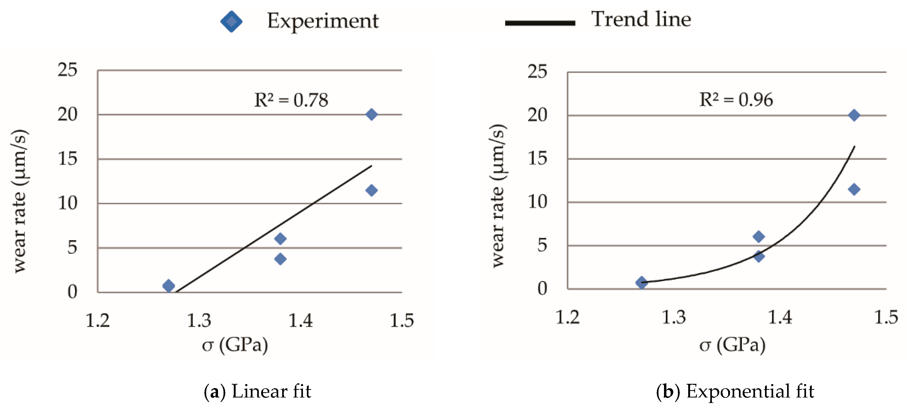
Based on the hypothesis that mechanical stresses are the main cause of tool wear in the initial period, a methodology was developed to predict the initial wear rate. First, the flank wear length and orientation with respect to time during initial cutting period, up to 100 µm, was measured. Orthogonal cutting process with no flank wear was then simulated and stress contour plot was obtained. Figure 11 shows the contour of Von Mises stresses in the tool for the lowest, mid-range and highest magnitudes of cutting parameters listed in Table 1. Following on from here, the measured flank wear length and orientation were superimposed onto the stress contour plot and average stress along the flank wear length was calculated. Dotted rectangles in Figure 11 show the flank area in the simulated tool where the stresses have been obtained Finally, the experimentally obtained wear rate in the initial period was related to the calculated average stress. Figure 12 shows the experimentally obtained wear rates, dW/dt, plotted against the simulated Von Mises stresses. Referring to the coefficient of determination, R², it was concluded that the exponential function fitted the relation better than the linear function. The equation representing the relation is detailed in Equation (5):

$$\mathrm{dW}/\mathrm{dt}=\mathrm{C}{\mathrm{e}}^{(\mathrm{D}\mathsf{\sigma })}$$

(5)

in which C and D are the constants to be determined through calibration. Employing the experimental and simulated data in Figure 12, the calibrated constants C and D were 1.26 × 10⁻⁹ µm/s and 1.59 × 10⁻⁸ m²/N, respectively.

Figure 13 compares the predicted wear rates when using Usui and newly proposed equation, with experimental results. In the five conditions analyzed, 0.75 to 5 µm/s differences between predictions and experiments were improved to 0.45 to 2 µm/s. The most significant improvement in the predicted wear rate was at 300 m/min cutting speed and 0.2 mm/rev feed rate. At this condition, Usui precited wear rate was 5.22 µm/s. However, with the proposed equation, the predicted wear rate was 12.42 µm/s which agrees better with the experimental data of 10.36 µm/s.

5.4. Wear Rate Predictions in the Secondary and Tertiary Cutting Periods

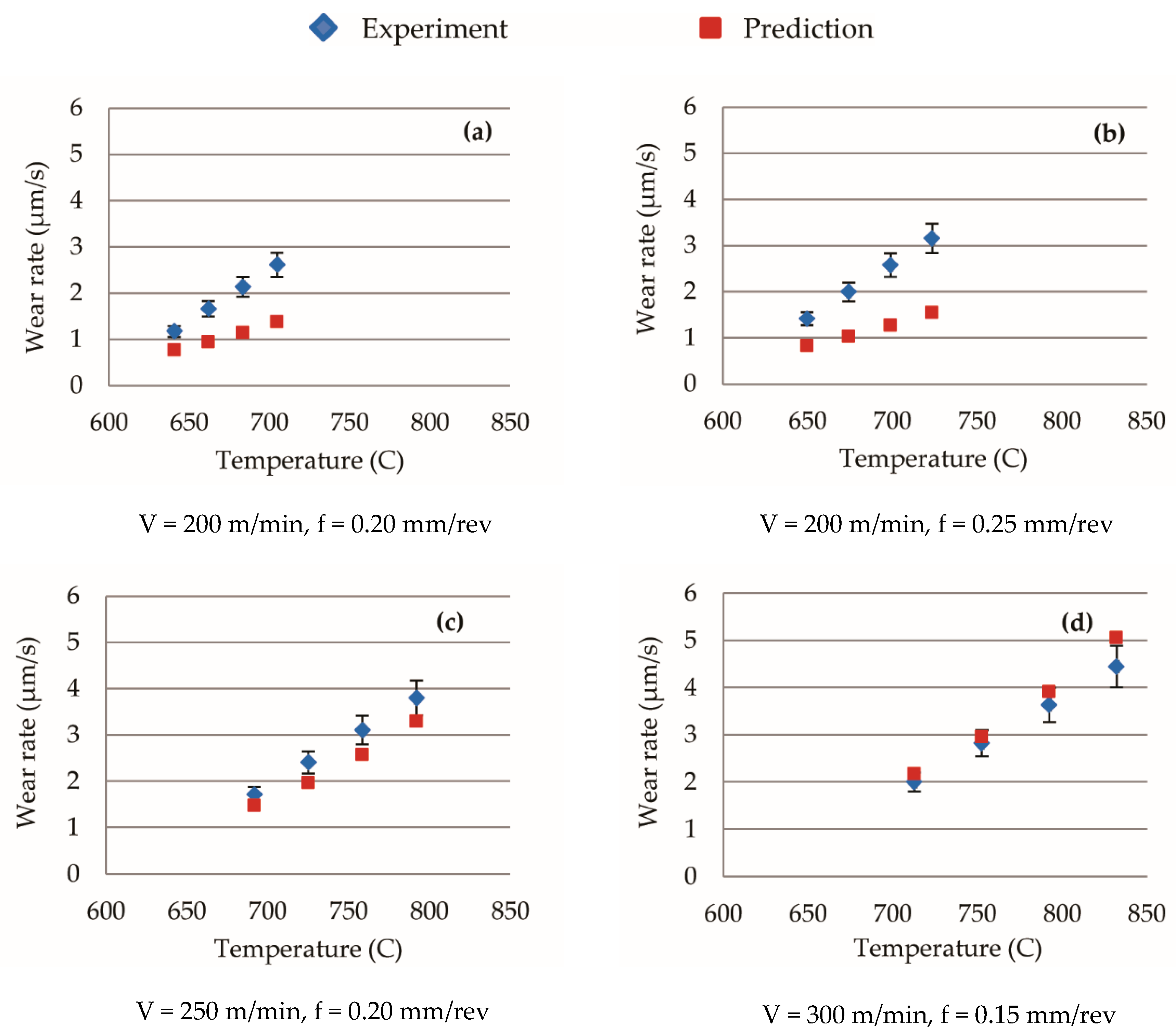
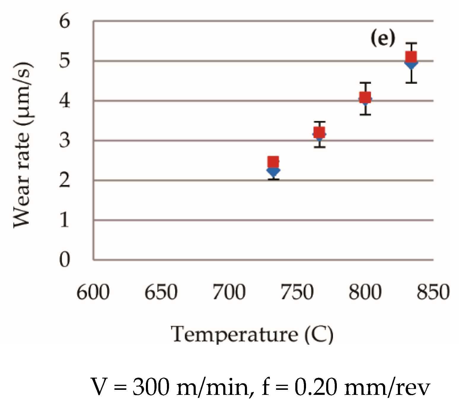
Figure 14 shows the effect of simulated temperature on tool wear rates acquired experimentally and predicted with Usui model for different cutting parameters during the secondary and tertiary tool life periods. The simulated temperatures along the flank face/ workpiece interface were compared to experimental results performed by Filice et al. [25]. The difference between predicted temperature and those acquired experimentally were less than 70 °C for two different sets of process parameter. With reference to Equation (2), wear rate is an exponential function of temperature. Zanger [13] showed that in the Usui model, the sensitivity of wear rate to temperature was much higher than to contact pressure and velocity. Therefore, in Figure 14, the estimated wear rates have been plotted with respect to the corresponding temperature. The four data points in each graph of Figure 14 represented the wear rates in 100–150 µm, 150–200 µm, 200–250 µm, and 250–300 µm flank wear intervals.

At 250 m/min and 300 m/min cutting speed, the wear rates were predicted in better agreement with experiments compared to the predictions in conditions with 200 m/min. In Figure 14a,b, for conditions with 200 m/min speed, the predicted wear rate was approximately 40% to 50% lower when compared to experiment. On the other hand, in Figure 14c–e, for conditions with higher speeds of 250 m/min and 300 m/min, wear rates at any flank wear interval were predicted within in ±20% when compared to experiment.

In the current FE simulations, the average temperature and pressure on the flank face were stable while instability was observed in the sliding velocity of work material passing over the tool face. As the result, the sliding velocity equivalent to cutting speed magnitude was used in the wear rate model instead of simulated sliding velocity. Malakizadi [16] observed similar instability in the sliding velocity and used cutting speed instead of sliding velocity.

In the next section a methodology is detailed to calculate the workpiece sliding velocity from strain field distribution and stable time increment.

5.5. Strain and Velocity Distributions Beneath the Newly Generated Surface

Figure 15 shows the predicted plastic strain distribution beneath the newly generated surface when the flank wear was at 200 µm. The plastic strain was parallel to the cutting velocity vector and the newly generated surface was still in contact with the flank face/workpiece interface. For all the cutting speed investigated, the plastic strain was at its maximum at the flank face/workpiece interface and decay to approximately zero at a depth of 15 µm. The high plastic strain induced on the surface was likely due to strain hardening effect when the material was fractured to form the chip or newly generated surface and also due to friction along the flank face/workpiece interface. Han et al. [25] also found similar trend during experimental orthogonal cutting test of annealed AISI 1045 with carbide tool. Experimentally acquired micrographs showed the surface with intense bending of the cementite plates within the pearlite phase and in some cases the formation of white layer. The white layers are generally formed due to rapid heating and cooling, severe plastic deformation and reaction of the surface with the environment. The bending of the cementite plates was observed up to a depth of less than 10 µm, which was similar to the depth predicted in Figure 15.

The cutting speed had no substantial effect in surface plastic strain. Han et al. [26] also made similar observation when increasing cutting speed on the thickness of formed white layer. Han et al. found that when cutting speed was increased from 100 to 200 m/min with a flank wear length of 100 µm, the formation of white layer measured depths were 1 µm to 2 µm, respectively, which is not a substantial difference. This shows that increased cutting speed has insignificant effect on the plastic strain induced on the newly generated surface.

Figure 16 details the simulated velocity distribution beneath the newly generated surface. This velocity is parallel to the cutting speed and was acquired in the region when the newly generated surface was still in contact with the flank face of the tool. The velocity distribution was calculated using the relative strain history distribution, ε_t(i) − ε_t(i-1), divided by the stable simulated time increment, t_S, and multiplied with the corresponding distance travelled, d_(i−1), as shown in Equation (6). This approach will eliminate any instability as observed here as well by Malakizadi [16].

$${\mathrm{v}}_{\mathrm{s}}=[({\epsilon }_{\mathrm{t}(\mathrm{i})}-{\epsilon }_{\mathrm{t}(\mathrm{i}-1)})/{\mathrm{t}}_{\mathrm{s}}]\times {\mathrm{d}}_{(\mathrm{i}-1)}$$

(6)

As expected, the velocity was lower near the newly generated surface. This was due to plastic deformation that occurs in the region as shown in Figure 15. Further away from the newly generated surface, the velocity increased to its prescribed cutting speed. At 7.5 µm depth beneath the flank face/workpiece interface, the velocity range bar overlapped one another regardless of the cutting speed simulated. At 10 µm depth, the range bar did not overlap. This was likely due to the contact interfaces were simulated with stick-slip condition, which is dependent on the normal pressure acting along the contacting surfaces. When the node undergoes a transition between sticking to slipping, the node will have high relative kinetic energy. In the sticking region, the difference between the sliding velocity and cutting velocity is high. In the slipping region, this difference was substantially reduced, and therefore the node will experience high kinetic energy resulting in oscillation of the predicted velocity. This was not observed when the depth of the newly generated surface was increased as no plastic deformation was observed.

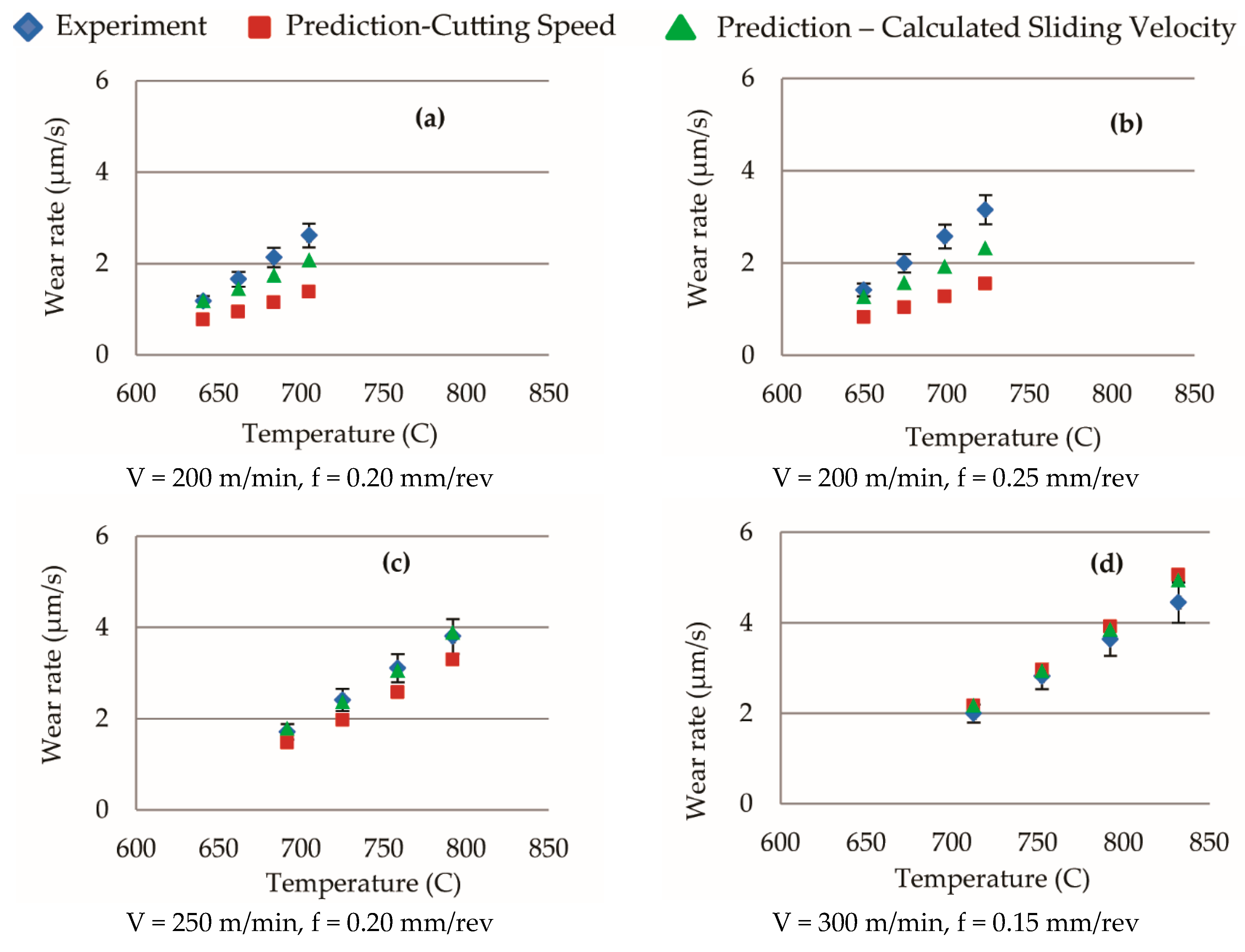
Therefore, it was concluded that the sliding velocity of 0.86 m/s, which was calculated by taking the average of the maximum and minimum velocity for all the cutting conditions simulated, could be used in the wear rate predictions.

Table 4. Model constants for the calibrated equation based on two boundary conditions.

Region	B1 (m2/MN)	B2 (°C)
Initial Period	9.14 × 10−5	7005
Secondary/Tertiary Periods	9.42 × 10−8	3135

shows the new calibrated constants based on using the constant sliding velocity of 0.86 m/s and Figure 17 shows the corresponding new predicted wear rates. The current approach of acquiring sliding velocity together with Usui model improved the wear rate predictions in all the conditions, especially in those with cutting speed of 200 m/min. The difference between predicted and experimental results at 200 m/min cutting speed was reduced to within 20% from 40% to 50%. The wear rate predictions at condition with 250 m/min and 300 m/min cutting speed was also reduced to 10% from 20%.

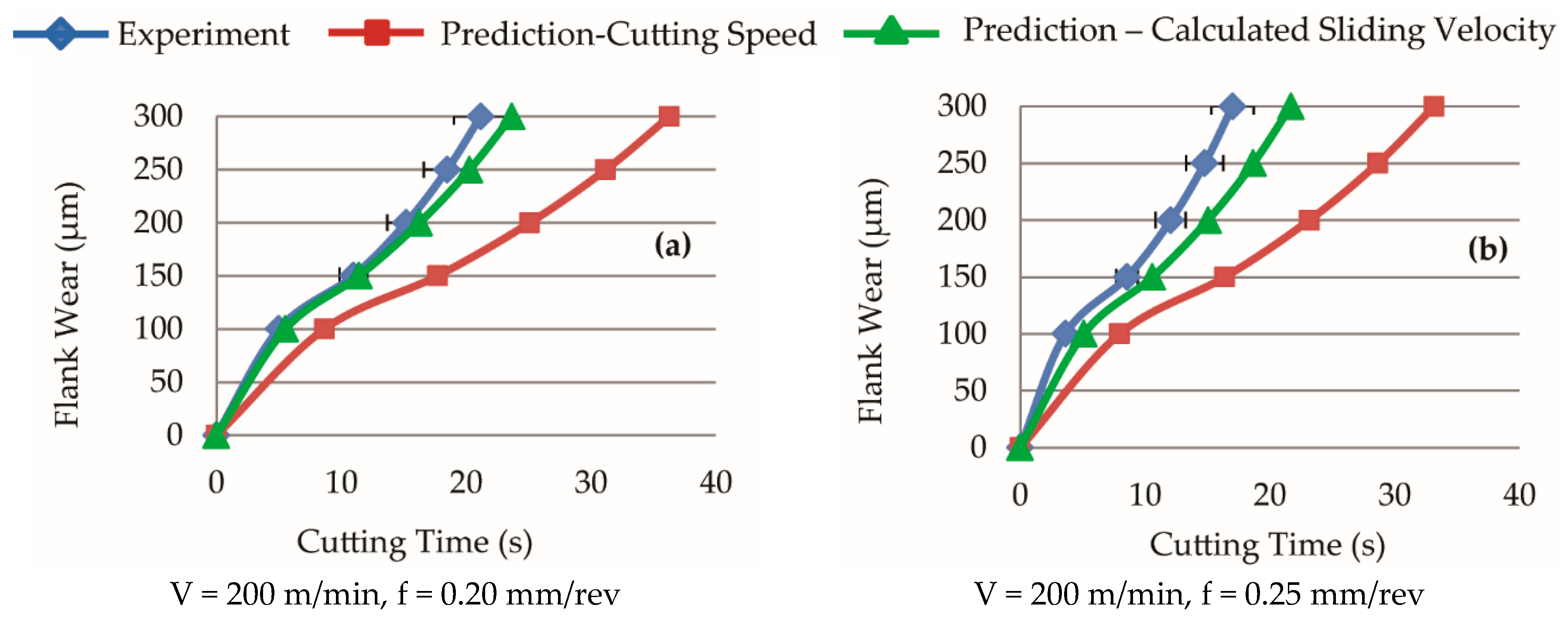
Figure 18a,b shows the tool life results from experiment, predictions when using cutting speed as sliding velocity, and predictions when using the 0.86 m/s calculated average sliding velocity. Tool life prediction agreed better with experiment when the calculated average sliding velocity was used. In this case, at cutting speed of 200 m/min together with feed rates of 0.20 mm/rev and 0.25 mm/rev, the difference between predicted tool life with experiment at 0.3 mm flank wear were approximately 14% and 20% respectively. However, when the cutting speed was assumed to be equal to the sliding velocity, the difference for both feed rates were between 73% and 110%. Similar trends were observed at the higher cutting speeds with corresponding feed rates.

5.6. Computational Time Improvement

Based on the current methodology proposed here, FE simulations with worn edge geometries were carried out in parallel, which were independent from each other. Simulations were completed when temperature and stresses reached study state. This approach substantially reduced the overall computation time when compared to the methodologies published by other researchers [12,14,17], where simulations were performed in series, as shown in Figure 1. Equation (7) shows the overall computational time when the series approach was used,

$$\mathrm{Computational} \mathrm{time} \mathrm{in} \mathrm{series}=({\mathrm{t}}_{\mathrm{p}}\times {\mathrm{t}}_{\mathrm{R}})/({\mathrm{t}}_{\mathrm{s}}\times {\mathrm{i}}_{\mathrm{s}})$$

(7)

where t_p is the time required to generate 0.3 mm flank wear, t_R is the real computational time for a specific number of increments, t_S is the stable time increment, and i_S is the specific number of increments. The computational time shown in Equation (7) is highly dependent on the time required to generate 0.3 mm flank wear.

The computational time in parallel that was developed in this research can be calculated using Equation (8),

$$\mathrm{Computational} \mathrm{time} \mathrm{in} \mathrm{parallel}=({\mathrm{t}}_{\mathrm{S}\mathrm{S}}\times {\mathrm{t}}_{\mathrm{R}}\times {\mathrm{n}}_{\mathrm{i}})/({\mathrm{t}}_{\mathrm{s}}\times {\mathrm{i}}_{\mathrm{s}})$$

(8)

where t_SS is the time taken for the cutting forces and cutting temperature to reach steady state and n_i is the number of wear intervals. The definition on the rest of the terms found in Equation (8) were similar to those listed in Equation (7).

The computation time in Equation (8) is substantially lower when compared to Equation (7), as the time taken for the cutting forces and temperature to reach steady state is dependent on the length of cut simulated divided by the cutting speed, whereas the time required to generate 0.3 mm flank wear using Equation (7) is dependent on the real tool wear rate.

Table 5. Effect of time required to generate 0.3 mm flank wear and computational time with series and parallel simulation.

	Computational Time in Series Approach, Equation (7)			Computational Time in Parallel Approach, Equation (8)
${\mathrm{t}}_{\mathrm{p}}$(s)	30	300	3000	30	300	3000
${\mathrm{t}}_{\mathrm{S}\mathrm{S}}$(s)				0.5	0.5	0.5
${\mathrm{t}}_{\mathrm{S}}$(s)	5 × 10−8	5 × 10−8	5 × 10−8	5 × 10−8	5 × 10−8	5 × 10−8
${\mathrm{i}}_{\mathrm{S}}$	250,000	250,000	250,000	250,000	250,000	250,000
${\mathrm{t}}_{\mathrm{R}}$(s)	120	120	120	120	120	120
${\mathrm{n}}_{\mathrm{i}}$	-	-	-	6	6	6
Actual computational time	0.28 × 106 s 4800 min	2.88 × 106 s 48,000 min	28.8 × 106 s 480,000 min	28.8 × 103 s 480 min	28.8 × 103 s 480 min	28.8 × 103 s 480 min

details the computational time calculation using Equations (7) and (8). When using series approach, the actual computational time increased with the time required to generate 0.3 mm flank wear, whereas with the parallel approach, which was developed in this research, the computational time was independent to tool wear rate. For example, when the time required to generate 0.3 mm flank wear was fixed at 30 s, the computation time for series approach was 10 times longer when compared to the method detailed in this paper.

6. Conclusions

In this paper, a hybrid finite element method coupled with empirical wear rate equation to predict tool life was presented and validated experimentally. The following conclusions were made based on the orthogonal cutting of AISI 1045 with uncoated carbide with the associated process parameters.

Experimental results showed that Usui’s equation had limitation predicting the tool wear rate during the initial tool wear period, which is dominated by mechanical stresses. A new empirical equation was proposed here which predict the initial tool wear rate as a function of Von Mises stress together with calibrated constants. Experimental validation showed evidence that the newly developed empirical equation substantially improved the predicted tool wear rate. The limitations of this approach were that a 100 μm initial flank wear length was assumed and empirical model calibration was required.

Due to the inherent instable of the sliding velocity from the stick-slip condition at the contacting surface, the relative strain history and stable simulated time increment was used to calculate the sliding velocity distribution beneath the newly generated surface. The average sliding velocity used at the tool/flank face interface for the cutting conditions investigated was 0.86 m/s. When using this sliding velocity magnitude, the tool wear rate and tool life predicted during the secondary and tertiary cutting periods agreed better with experimental results regardless of cutting speed or tool wear life.

In the current research approach, the FE computational time was significantly reduced. This reduction was due to the fact that the FE simulation with different flank wear lengths could be computed in parallel and for each flank wear length interval, the simulated cutting time is dependent on the duration when the mechanical and thermal field becomes steady state. When using the nodal movement technique together with series approach, the FE computational time is coupled to the tool wear rate, which can have long computational time. However, there are also two limitations is the current approach, which are (i) the angle between the rake face and flank face must not vary with tool life and (ii) at least two sets of experiments are required for model calibration.

References

1. Taylor, F.W. On the art of cutting metals. Trans. Am. Soc. Mech. Eng. 1907, 28, 31–58. [Google Scholar]
2. Li, B. A review of tool wear estimation using theoretical analysis and numerical simulation technologies. Int. J. Refract. Met. Hard Mater. 2012, 35, 143–151. [Google Scholar] [CrossRef]
3. Shaw, M.C.; Dirke, S.O. On the wear of cutting tools. Microtecnic 1956, 10, 187–193. [Google Scholar]
4. Trigger, K.J.; Chao, B.T. The mechanism of crater wear of cemented carbide tools. Trans. ASME 1956, 78, 1119. [Google Scholar]
5. Usui, E.; Shirakashi, T.; Kitagawa, T. Analytical prediction of cutting tool wear. Int. J. Wear 1984, 100, 129–151. [Google Scholar] [CrossRef]
6. Kitagawa, T.; Maekawa, K.; Shirakashi, T.; Usui, E. Analytical prediction of flank wear of carbide tools in turning plain carbon steels, part 1: Characteristic equation of flank wear. Bull. Japan Soc. Prec. Eng. 1988, 22, 263–269. [Google Scholar]
7. Maekawa, K.; Kitagawa, T.; Shirakashi, T.; Usui, E. Analytical prediction of flank wear of carbide tools in turning plain carbon steels, part 2: Prediction of flank wear. Bull. Japan Soc. Prec. Eng. 1989, 23, 126–133. [Google Scholar]
8. Denkena, B.; Köhler, J.; Mengesha, M.S. Influence of the cutting edge rounding on the chip formation process: Part 1. Investigation of material flow, process forces, and cutting temperature. Prod. Eng. 2012, 6, 329–338. [Google Scholar] [CrossRef]
9. Sanchez, A.M.; Canteli, J.A.; Cantero, J.L.; Miguelez, M.H. Numerical analysis of tool wear effect in machining induced residual stresses. Simul. Model. Pract. Theory 2011, 19, 872–886. [Google Scholar] [CrossRef] [Green Version]
10. Yen, Y.C.; Söhner, J.; Lilly, B.; Altan, T. Estimation of tool wear in orthogonal cutting using the finite element analysis. J. Mater. Process. Technol. 2004, 146, 82–91. [Google Scholar] [CrossRef]
11. Xie, L.-J.; Schmidt, J.; Schmidt, C.; Biesinger, F. 2D FEM estimate of tool wear in turning operation. Int. J. Wear 2005, 258, 1479–1490. [Google Scholar] [CrossRef]
12. Filice, L.; Micari, F.; Settineri, L.; Umbrello, D. Wear modelling in mild steel orthogonal cutting when using uncoated carbide tools. Int. J. Wear 2007, 262, 545–554. [Google Scholar] [CrossRef]
13. Zanger, F.; Schulze, V. Investigation on Mechanisms of Tool Wear in Machining of Ti-6Al-4V using FEM Simulation. Procedia CIRP 2013, 8, 158–163. [Google Scholar] [CrossRef] [Green Version]
14. Attanasio, A.; Ceretti, E.; Fiorentino, A.; Cappellini, C.; Giardini, C. Investigation and FEM-based simulation of tool wear in turning operations with uncoated carbide tools. Int. J. Wear 2010, 269, 344–350. [Google Scholar] [CrossRef]
15. Attanasio, A.; Ceretti, E.; Giardini, C. 3D FEM Simulation of Flank Wear in Turning. In Proceedings of the 14th International ESAFORM Conference on Material Forming, Belfast, UK, 27–29 April 2011; pp. 561–566. [Google Scholar]
16. Malakizadi, A.; Gruber, H.; Sadik, I.; Nyborg, L. An FEM-based approach for tool wear estimation in machining. Int. J. Wear 2016, 368–369, 10–24. [Google Scholar] [CrossRef]
17. Malakizadi, A.; Cedergren, S.; Surreddi, K.B.; Nyborg, L. A methodology to evaluate the machinability of Alloy 718 by means of FE simulation. In Proceedings of Advanced Manufacturing Engineering and Technologies; NEWTECH: Stockholm, Sweden, 2013; pp. 95–106. [Google Scholar]
18. Hosseinkhani, K.; Ng, E. A Combined Empirical and Numerical Approach for Tool Wear Prediction in Machining. Procedia CIRP 2015, 31, 304–309. [Google Scholar] [CrossRef]
19. Lane, B.M.; Dow, T.A.; Scattergood, R. Thermo-chemical wear model and worn shapes for single-crystal diamond tools cutting steel. Int. J. Wear 2013, 300, 216–224. [Google Scholar] [CrossRef]
20. Hosseinkhani, K.; Ng, E. Analysis of the cutting mechanics under the influence of worn tool geometry. Procedia CIRP 2013, 8, 117–122. [Google Scholar] [CrossRef] [Green Version]
21. Hosseinkhani, K.; Ng, E. A hybrid experimental and simulation approach to evaluate the calibration of tool wear rate models in machining. Int. J. Adv. Manuf. Technol. 2018, 96, 2709–2724. [Google Scholar] [CrossRef]
22. Shaw, M.C. Metal Cutting Principles, 2nd ed.; Oxford University Press Inc.: Oxford, UK, 2005. [Google Scholar]
23. Binder, M.; Klocke, F.; Doebbeler, B. An advanced numerical approach on tool wear simulation for tool and process design in metal cutting. Simul. Model. Pract. Theory 2017, 70, 65–82. [Google Scholar] [CrossRef]
24. Palmai, Z. Proposal for a new theoretical model of the cutting tool’s flank wear. Int. J. Wear 2013, 303, 437–445. [Google Scholar] [CrossRef]
25. Filice, L.; Umbrello, D.; Beccasri, S.; Micari, F. On the FE Codes Capability for Tool Temperature Calculation in Machining Processes. J. Mater. Process. Technol. 2006, 174, 286–292. [Google Scholar] [CrossRef]
26. Han, S.; Melkote, S.N.; Haluska, M.S.; Watkinsc, T.R. White Layer Formation Due to Phase Transformation in Orthogonal Machining of AISI 1045 Annealed Steel. Mater. Sci. Eng. 2008, 488, 195–204. [Google Scholar] [CrossRef]
Figure 1. Conventional tool wear prediction approach using finite element method and empirical wear rate equation.
Jmmp 04 00016 g001
Figure 2. Schematic of orthogonal cutting process.
Jmmp 04 00016 g002
Figure 3. Cutting conditions in the range of cutting parameters.
Jmmp 04 00016 g003
Figure 4. Schematics of edge geometries: (a) non-worn and (b) worn edge geometries.
Jmmp 04 00016 g004
Figure 5. Geometry of worn edges after machining first (ac) and last (df) fin with the lowest, mid-range, and highest process parameters.
Jmmp 04 00016 g005aJmmp 04 00016 g005b
Figure 6. Overall procedure of the proposed methodology.
Jmmp 04 00016 g006
Figure 7. (a) Geometry and boundary conditions of orthogonal Arbitrary Lagrangian–Eulerian (ALE) cutting models. (b) Chip formation in orthogonal ALE simulation: temperature, contact pressure, and sliding velocity at flank wear–workpiece interface.
Jmmp 04 00016 g007
Figure 8. Schematic of wear rate calculation in a flank wear interval.
Jmmp 04 00016 g008
Figure 9. Predicted tool life in comparison with experimental results.
Jmmp 04 00016 g009
Figure 10. Wear rates predictions corresponding to the initial cutting period.
Jmmp 04 00016 g010
Figure 11. Contour of Von Mises stresses developed in the tool cutting edge when machining at different cutting conditions.
Jmmp 04 00016 g011
Figure 12. Relation between the experimental wear rate in the initial cutting period and the simulated Von Mises stresses.
Jmmp 04 00016 g012
Figure 13. Predictions of wear rate in the initial period of cutting based on original Usui and new equations.
Jmmp 04 00016 g013
Figure 14. Effect of temperature on tool wear rates acquired experimentally and predicted with Usui model for different cutting parameters.
Jmmp 04 00016 g014aJmmp 04 00016 g014b
Figure 15. Effect of cutting speed on predicted plastic strain distribution beneath newly generated surface.
Jmmp 04 00016 g015
Figure 16. Velocity distribution beneath the newly generated surface.
Jmmp 04 00016 g016
Figure 17. Predicted wear rate according to the modified Usui model in comparison with experiment.
Jmmp 04 00016 g017aJmmp 04 00016 g017b
Figure 18. Predicted tool life according to original Usui and modified Usui in comparison with experiment.
Jmmp 04 00016 g018