Abstract
This paper describes a sample partitioning approach to retain or reject samples from an initial distribution of stability maps using milling test results. The stability maps are calculated using distributions of uncertain modal parameters that represent the tool tip frequency response functions and cutting force model coefficients. Test points for sample partitioning are selected using either (1) the combination of spindle speed and mean axial depth from the available samples that provides the high material removal rate, or (2) a spindle speed based on the chatter frequency and mean axial depth at that spindle speed. The latter is selected when an unstable (chatter) result is obtained from a test. Because the stability model input parameters are also partitioned using the test results, their uncertainty is reduced using a limited number of tests and the milling stability model accuracy is increased. A case study is provided to evaluate the algorithm.
1. Introduction
For discrete part production by milling, the optimum combination of spindle speed and axial depth is desired to maximize material removal rate (MRR) and minimize cost. To identify the optimal {spindle speed, axial depth} combination that provides maximum MRR without chatter (a self-excited vibration), analytical and numerical milling models are available [1]. These models have two primary inputs: (1) the tool tip frequency response function, FRF; and (2) a cutting force model that relates the cutting force to the commanded chip area using mechanistic coefficients. The tool tip FRF may be measured using tap testing, where an instrumented hammer is used to excite the tool tip and a linear transducer, such as a low-mass accelerometer, is used to measure the response [2,3,4]. The measured tool tip FRF can then be represented by a discrete number of vibration modes, each of which is described by a natural frequency, modal stiffness, and modal damping ratio. The cutting force model coefficients may be identified experimentally by measuring the cutting force for known milling parameters and determining the least-squares best fit coefficients using the force model and measured force [3,5].
The objective of this research is to increase milling stability model accuracy when the inputs are initially uncertain. Uncertainties in two inputs are considered: the modal parameters that represent the tool tip FRFs and the cutting force model coefficients. This paper is organized as follows. The sample partitioning approach is described that reduces uncertainty in the modal parameters and cutting force model coefficients using stability tests. Next, a case study is presented to evaluate the approach where the changes in initial model input distributions and corresponding stability boundaries are reported. Then, a discussion of the results is provided. Finally, conclusions are presented.
2. Sample Partitioning
A sample partitioning approach is proposed to reduce uncertainty in (1) the modal parameters that represent the tool tip FRF; and (2) the cutting force model coefficients using milling stability tests. The approach is to partition stability maps that agree with sequential stability tests completed at selected {spindle speed, axial depth} combinations from those that disagree. The stability maps are generated using the zero-order frequency domain stability model [6]. Tests are performed using time domain simulation, where the time-delay differential equations of motion that represent the milling system are solved numerically [3,7,8,9]. Because the zero-order frequency domain stability model inputs (i.e., the modal parameters and cutting force coefficients) are uncertain, Monte Carlo simulation is applied to randomly sample distributions of the inputs to predict many potential stability maps [10,11,12]. Each stability map represents one sample that may or may not be the true map; all samples have an equal probability of being the true stability map.
The selection of test points is based on the outcome of the previous test (i.e., stable or unstable/chatter behavior is exhibited). If the previous test was stable, the next test is selected where maximum expected MRR is obtained. To determine the test point in this case, the mean axial depth from all available stability maps (after partitioning based on the previous stable result) is identified for each spindle speed. The MRR is then calculated using the mean axial depth at the selected spindle speed. After repeating the calculation for each spindle speed, the {spindle speed, axial depth} combination that gives the maximum MRR is chosen as the next test point.
If the previous test is unstable, the chatter frequency is determined by converting a time domain milling signal, such as force or displacement, to the frequency domain. In the frequency domain, chatter is identified when content appears at frequencies other than the tooth passing frequency, ftooth, and its multiples (harmonics); see Equation (1), where Ω is the spindle speed (rpm) and Nt is the number of teeth on the endmill. The chatter frequency, fc (Hz), is applied to calculate the next spindle speed, Ω (rpm), using Equation (2) [13]. By comparing Equations (1) and (2), it is observed that the spindle speed for the next test is selected by setting the new tooth passing frequency equal to the chatter frequency from the previous test.
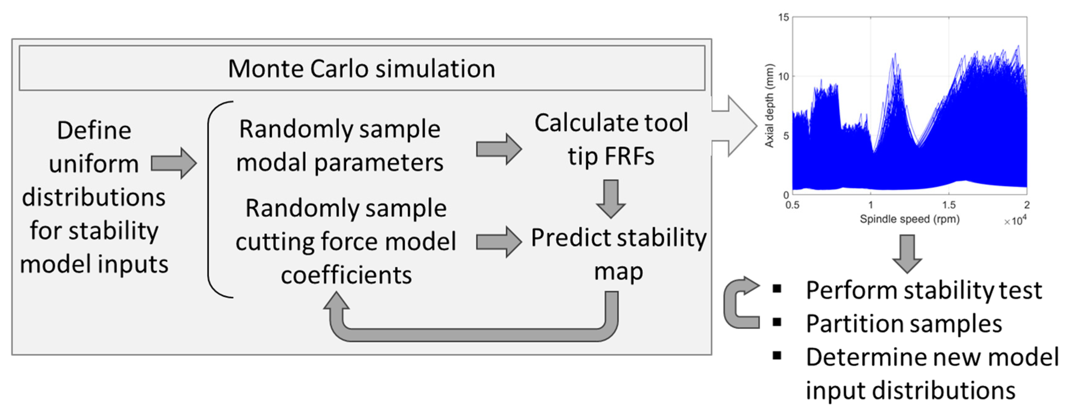
After partitioning the maps based on stability tests (i.e., a binary stable or unstable result is obtained), those maps that agree with the tests are used to identify the most likely input values and reduce the associated uncertainty since there is a one-to-one correspondence between the maps and the modal parameters and cutting force model coefficients. The approach is summarized in Figure 1.
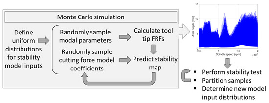
Figure 1.
Sample partitioning using stability testing.
2.1. Frequency Domain Stability Model
Altintas and Budak transform the dynamic milling equations into a time-invariant, radial immersion-dependent system [6]. They approximate the time-dependent cutting forces with an average value by expanding the time-varying coefficients of the dynamic milling equations, which depend on the angular orientation of the tool as it rotates through the cut, into a Fourier series. They then truncate the series to include only the average component and obtain an analytical solution for the limiting axial depth of cut to avoid chatter as a function of spindle speed. As noted, the two primary inputs to the analysis are the tool tip FRFs in the x (feed) and y directions and the coefficients for the mechanistic cutting force model.
2.2. Modal Parameters
The tool tip FRFs can be represented as a discrete number of vibration modes using modal analysis, where each mode is represented as a single-degree-of-freedom spring–mass–damper system [2,3,14,15,16]. The dynamic behavior of the spring–mass–damper system may be described using a natural frequency, fn (Hz), modal stiffness, k (N/m), and modal damping ratio, ζ (-). Any number of modes may be modeled using this approach.
2.3. Cutting Force Model
The resultant cutting force, F, and the tangential, Ft, and normal, Fn, direction components are shown in Figure 2 [3,5,17,18,19,20]. The expressions for Ft and Fn are given by Equations (3) and (4), where kt and kn are the cutting force coefficients, b is the axial depth (chip width), and h is the chip thickness.
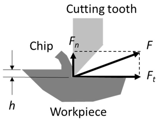
Figure 2.
Cutting force model.
2.4. Sample Partitioning Algorithm
The sample partitioning algorithm is described by Figure 3, which displays many potential stability boundaries (i.e., the family of blue curves) generated by Monte Carlo simulation. Consider the test at the {spindle speed, axial depth} pair labeled {Ωu, bu}. As indicated by the u subscript and the red ×, the test result is unstable. The stability boundaries are partitioned using this test result. Those that predict an unstable result (agree) are separated from those that predict a stable result (disagree). Only those sample boundaries that agree are retained. This means that all boundaries with a limiting axial depth greater than bu are eliminated from the distribution.
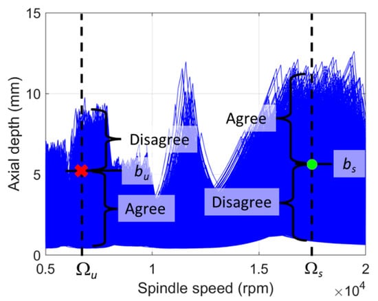
Figure 3.
Sample partitioning algorithm description. A red × indicates an unstable result and a green circle indicates a stable result.
Next, consider the test at {Ωs, bs}. As indicated by the s subscript and the green circle, the test result is stable. In this case, all boundaries with a limiting axial depth greater than bs at Ωs are retained (agree) and boundaries with a limiting axial depth less than bs at Ωs are eliminated (disagree) from the distribution. The sample partitioning is repeated sequentially for all tests, both stable and unstable, to refine the initial distributions of not only the stability maps, but also the modal parameters and cutting force model coefficients. Specifically, each map that disagrees with the test result and is eliminated also eliminates the corresponding values of the modal parameters and cutting force model coefficients used to produce that map. This enables the initial distributions of these uncertain parameters (stability model inputs) to be refined and, subsequently, the uncertainty in the parameters and stability predictions to be reduced.
2.5. Case Study
To evaluate the proposed sample partitioning algorithm and test selection approach, a numerical study was completed where the stability maps were predicted using the frequency domain stability model [6] and test data were collected using the results of milling time domain simulation [3]. For the milling stability tests, a 12.7 mm diameter, four-tooth endmill with a 30 deg helix angle and uniform teeth spacing was selected. The radial depth was 3 mm and the feed per tooth was 0.1 mm for the down milling, x-direction milling tests; the spindle speed and axial depth were varied to partition the predicted stability maps using the test results (labeled stable or unstable). The true modal parameters are provided in Table 1; two modes were selected and the FRFs were symmetric in the x and y directions. The true cutting force coefficients are also listed in Table 1; these are representative of a 6061-T6 aluminum workpiece material.

Table 1.
True values for stability model inputs.
Stability was determined using the x-direction displacement predicted by the time domain simulation. The time-dependent displacement was converted to the frequency domain and the chatter frequency was identified, if present. As noted, the frequency content from each test was compared to the tooth passing frequency (i.e., the spindle speed multiplied by the number of flutes) and its integer multiples (harmonics). A test was labeled as stable if content appeared only at these frequencies. A test was labeled as unstable if frequency content was observed at a different frequency and the chatter frequency was recorded for the selection of the next test point [21].
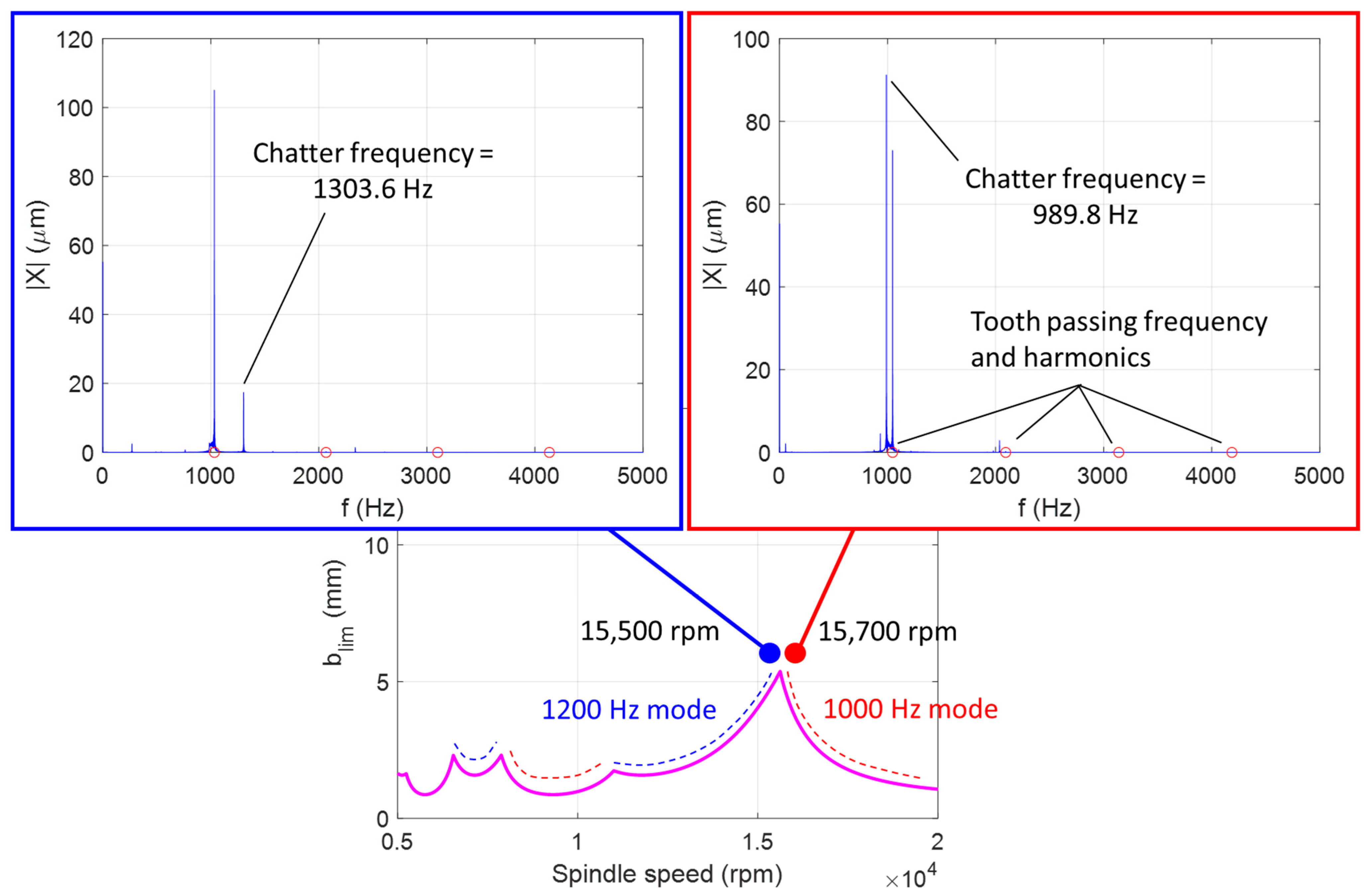
For the two-mode system, chatter can occur either in the 1000 Hz mode or the 1200 Hz depending on which portion of the stability boundary is exceeded. This is demonstrated in Figure 4, where it is observed that exceeding the stability boundary to the right of the peak at 15,620 rpm results in a different chatter frequency than exceeding the boundary to the left [22].
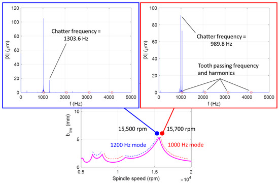
Figure 4.
Variation in chatter frequency with spindle speed and portion of the stability boundary that is exceeded. The stability map is shown at the bottom, where blim is the limiting axial depth to avoid chatter, and the insets show the frequency-dependent magnitude of the x-direction displacement for the two spindle speeds. The tooth passing frequency and its harmonics are identified by the open red circles.
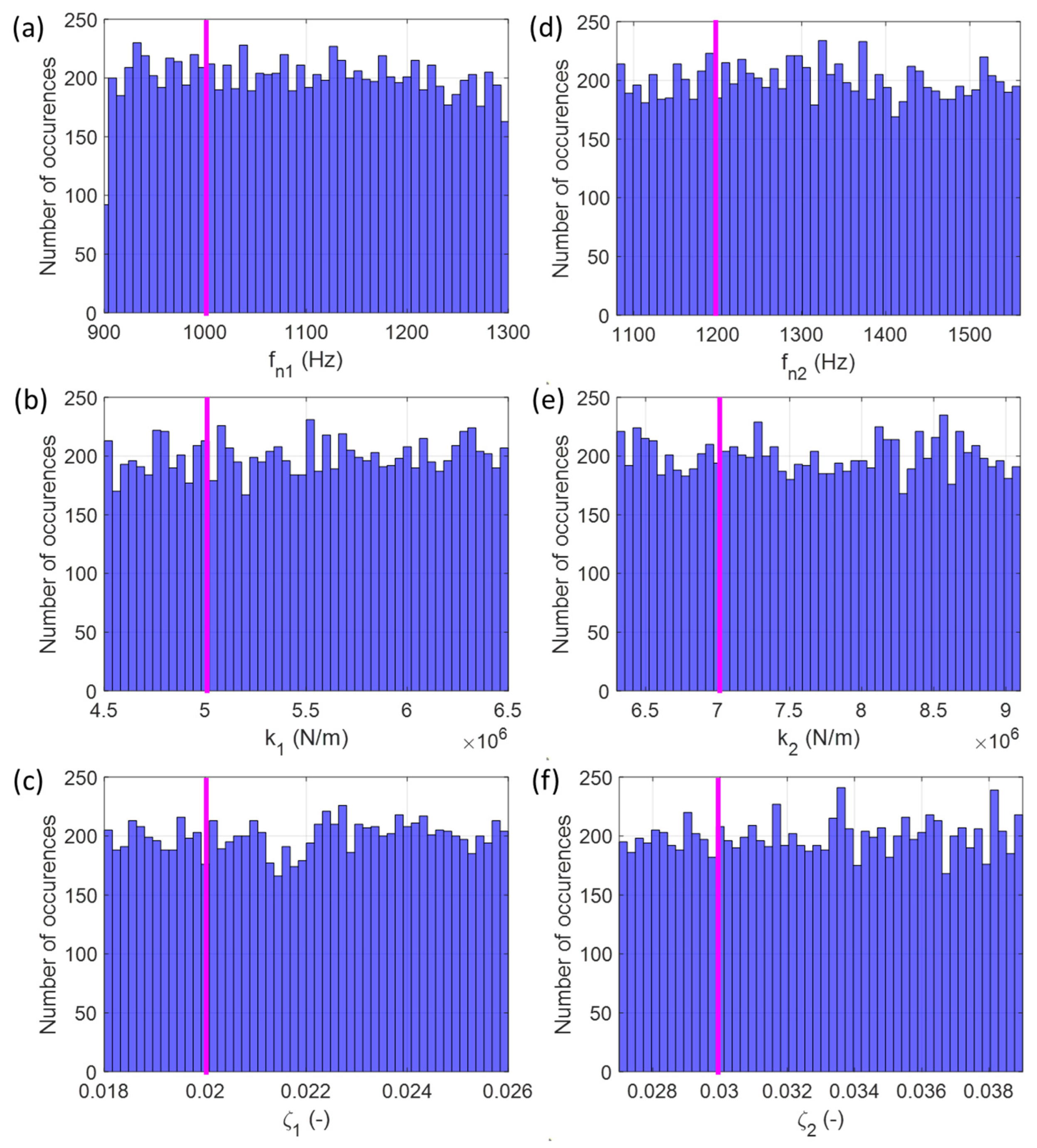
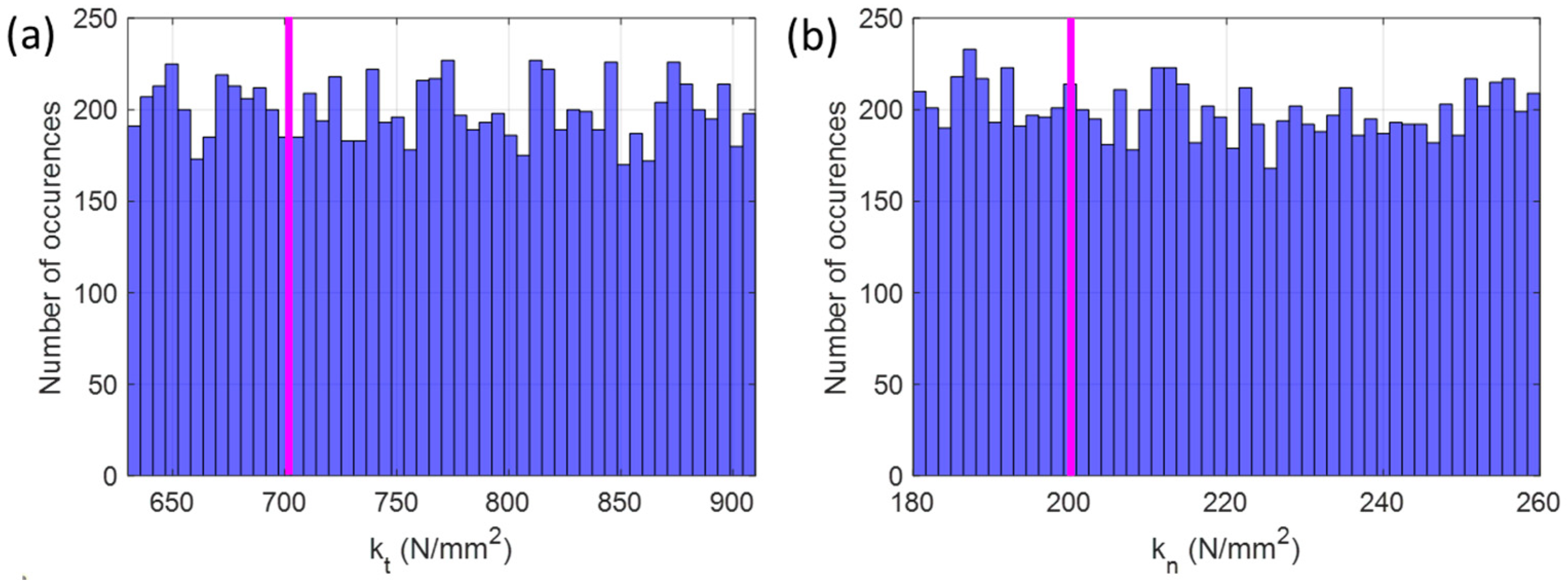
The initial uniform distributions for the Monte Carlo simulation were defined in the range from 90% of the input variable true value, T, to 130% of T, or U(0.9T, 1.3T) [23]. This approach was selected so that (1) each sample was equally likely to represent the true input value and (2) the true value was not located at the center of the distribution range. See Figure 5 and Figure 6, where the horizontal axis ranges from 0.9T to 1.3T in each case and the true value is identified.
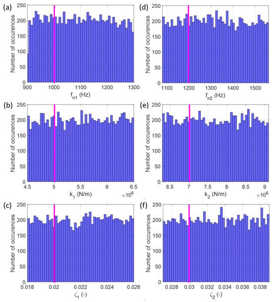
Figure 5.
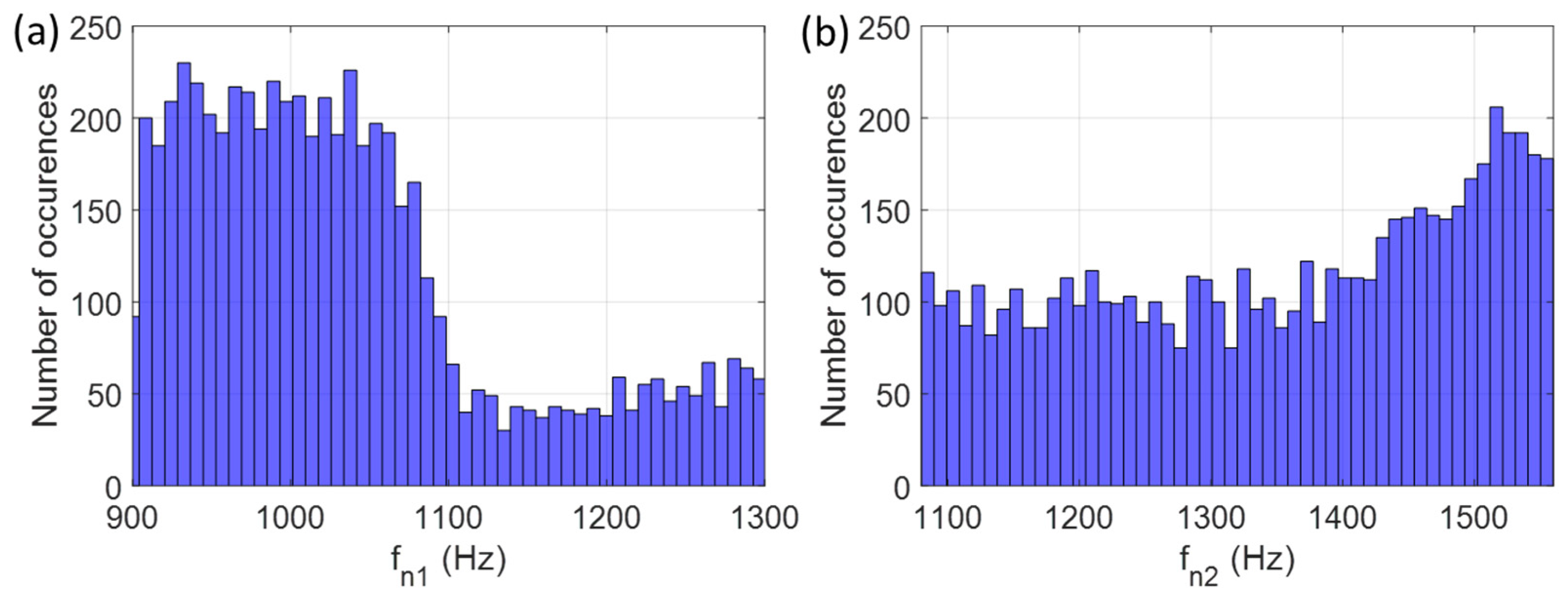
Initial distributions of (a) fn1; (b) k1; (c) ζ1; (d) fn2; (e) k2; and (f) ζ2. The histograms include 50 bins with 1 × 10⁴ samples, so there are approximately 200 samples per bin. The magenta lines identify the true values.
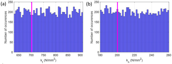
Figure 6.
Initial distributions of (a) kt and (b) kn. The magenta lines identify the true values.
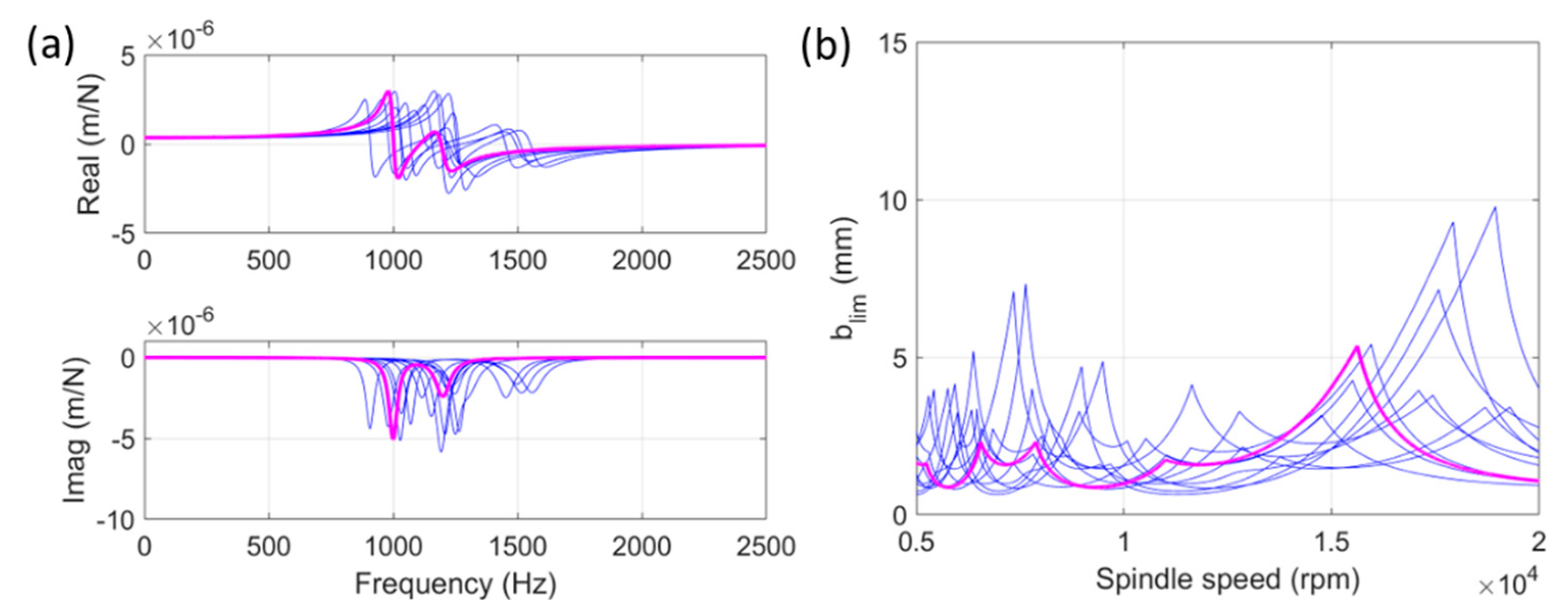
The six modal parameter distributions were randomly sampled to generate the symmetric tool tip FRFs; see Equation (5), where f is the excitation frequency (Hz) and Fx is the cutting force in the x direction [3]. The cutting force coefficient distributions were then sampled and combined with the tool tip FRFs to generate 1 × 10⁴ stability maps using the zero-order frequency domain model [6]. The eight input parameters were assumed to be uncorrelated. The distributions of 10 FRFs and stability maps are shown in Figure 7 to observe the variation obtained from the Monte Carlo simulation.

Figure 7.
Distributions of 10 (a) FRFs and (b) stability maps. The real and imaginary parts of the FRF and the stability map obtained from the true values in Table 1 are identified by magenta curves.
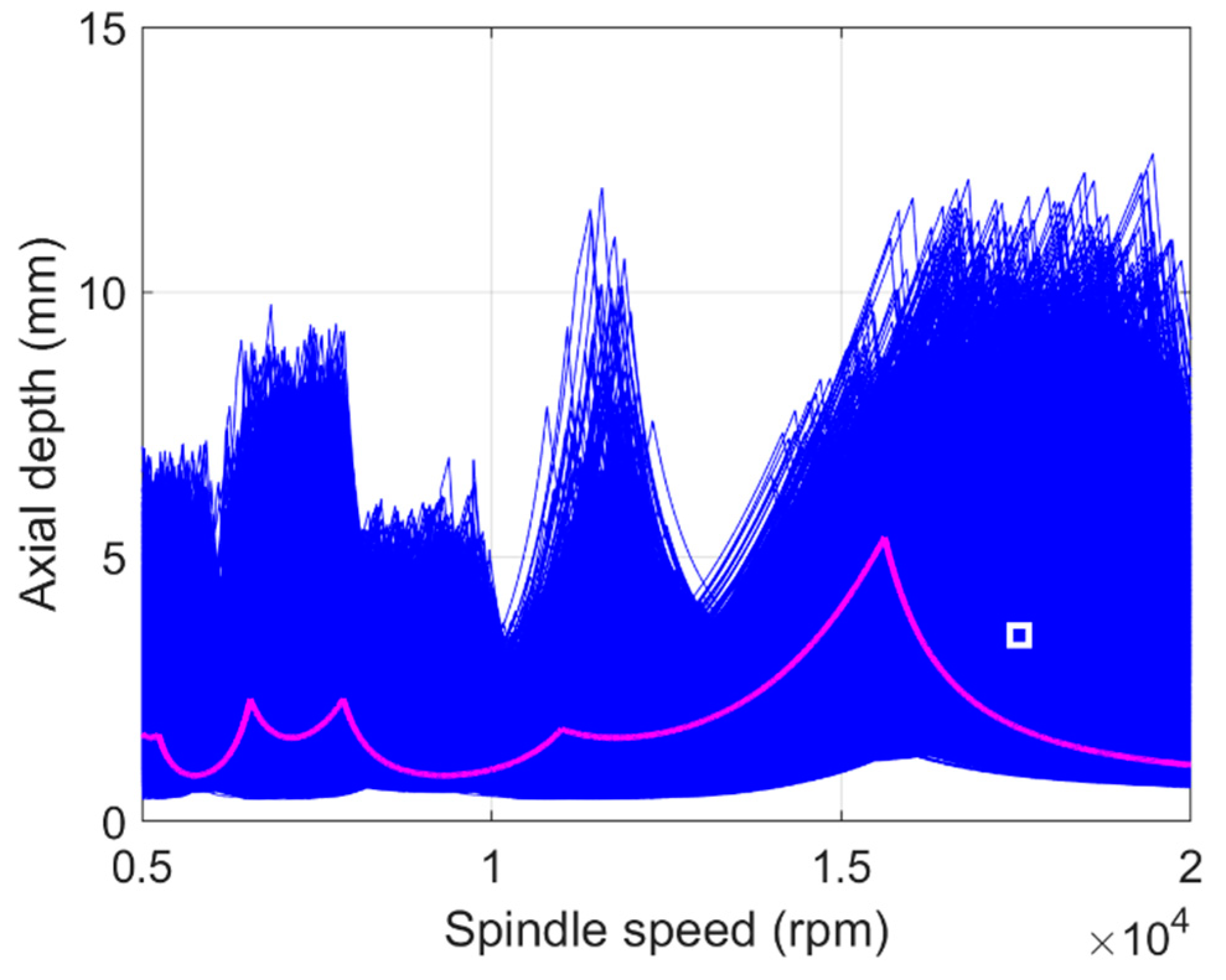
Given the 1 × 10⁴ initial stability maps obtained by Monte Carlo simulation, the first test point was selected using the maximum MRR criterion [24]. The result is displayed in Figure 8, where the spindle speed is 17,547 rpm and the axial depth is 3.5082 mm. This maximum expected MRR test point is marked by a white square. The stability map obtained from the true model input values (Table 1) is also indicated by a magenta curve. This is provided as a reference because it is not known at the time of testing and, therefore, does not influence the test point selection.

Figure 8.
Initial distribution of stability maps (blue curves) and first test point (white square). The stability map obtained from the true model input values is included as the magenta curve.
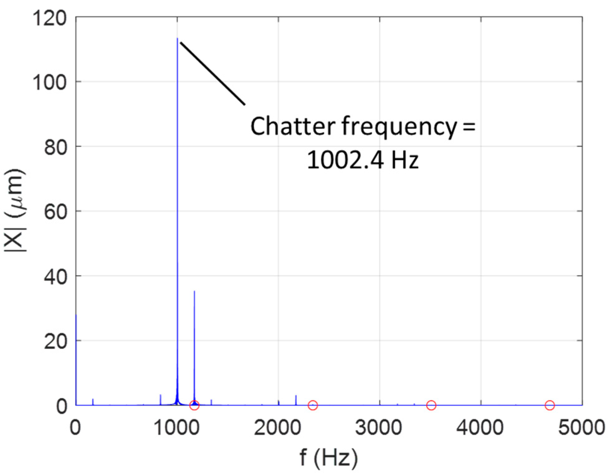
The first test point identified in Figure 8 is unstable. The corresponding chatter frequency of 1002.4 Hz is identified in Figure 9. The sample partitioning result is displayed in Figure 10, where it is observed that all stability boundaries below the test point are eliminated. In Figure 8, 5933 samples remain after partitioning. The new distributions in fn1 and fn2 are displayed in Figure 11. Because chatter occurred in the 1000 Hz mode, the fn1 distribution accuracy was increased significantly (i.e., those natural frequencies that were far from the true value were effectively eliminated). No appreciable change was observed for the other six distributions (i.e., they remained approximately uniform).
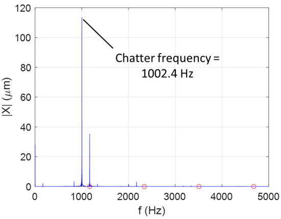
Figure 9.
Frequency content of the x-direction tool displacement for the {17,547 rpm, 3.5082 mm} test point. The test is unstable and the chatter frequency is 1002.4 Hz.

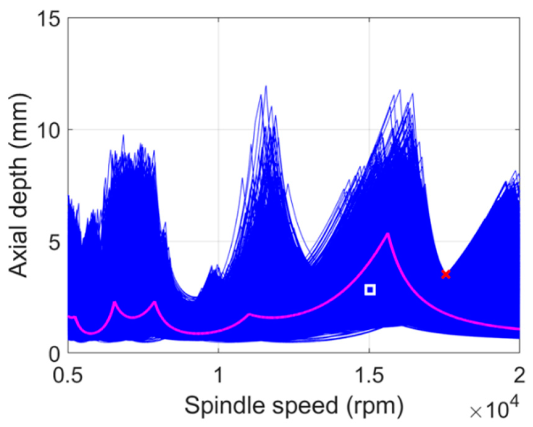
Figure 10.
Remaining stability maps (5933) after the unstable test at {17,547 rpm, 3.5082 mm}; the test point is marked by the red ×. The second test point is identified by a white square.
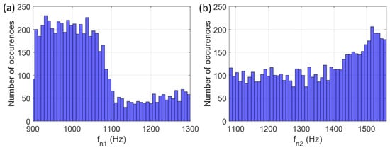
Figure 11.
Distribution of 5933 remaining natural frequencies after the first test: (a) fn1 and (b) fn2. The horizontal axis ranges are identical to Figure 5.
Given the unstable test and corresponding chatter frequency of 1002.4 Hz, the spindle speed for the second test was calculated using Equation (2). Specifically, rpm. The mean limiting axial depth at the selected spindle speed from the remaining stability maps was 2.8313 mm. The second test point is marked by a white square in Figure 10.
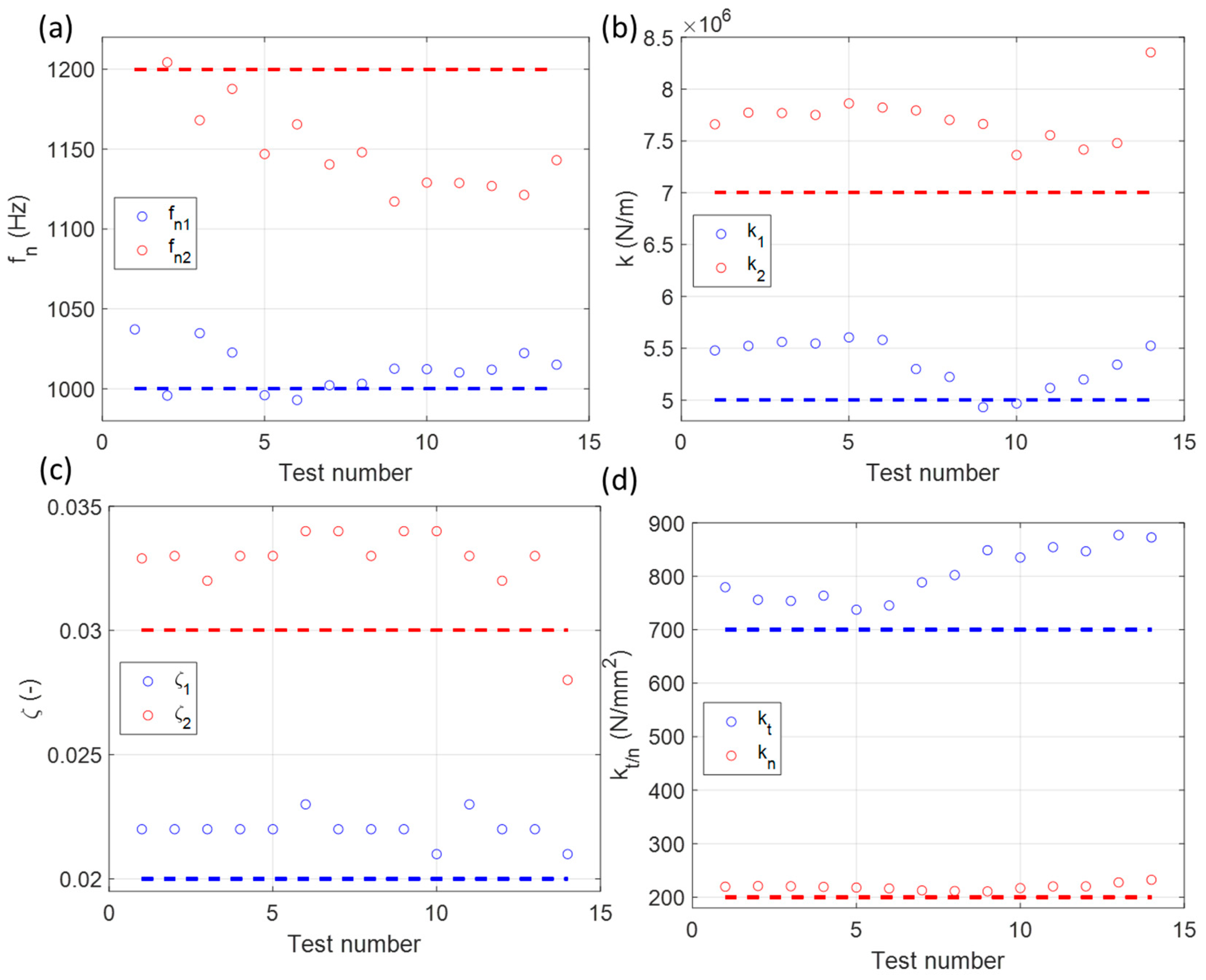
This test and partition sequence was repeated 14 times until only a single stability map remained. The test points, number of samples remaining after each test, and the chatter frequency, if present, are reported in Table 2. The corresponding mean values of the stability model input parameters after each test are provided in Table 3 and displayed in Figure 12 as a function of the test number.
Table 2.
Testing and sample partitioning results.
Table 3.
Mean values of the stability model input parameters after each test.
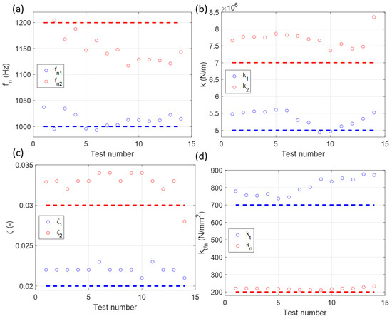
Figure 12.
Mean values of the stability model input parameters as a function of test number (a) natural frequency (b) stiffness (c) damping ratio (d) cutting force coefficients. The true values are indicated by the horizontal dashed lines.
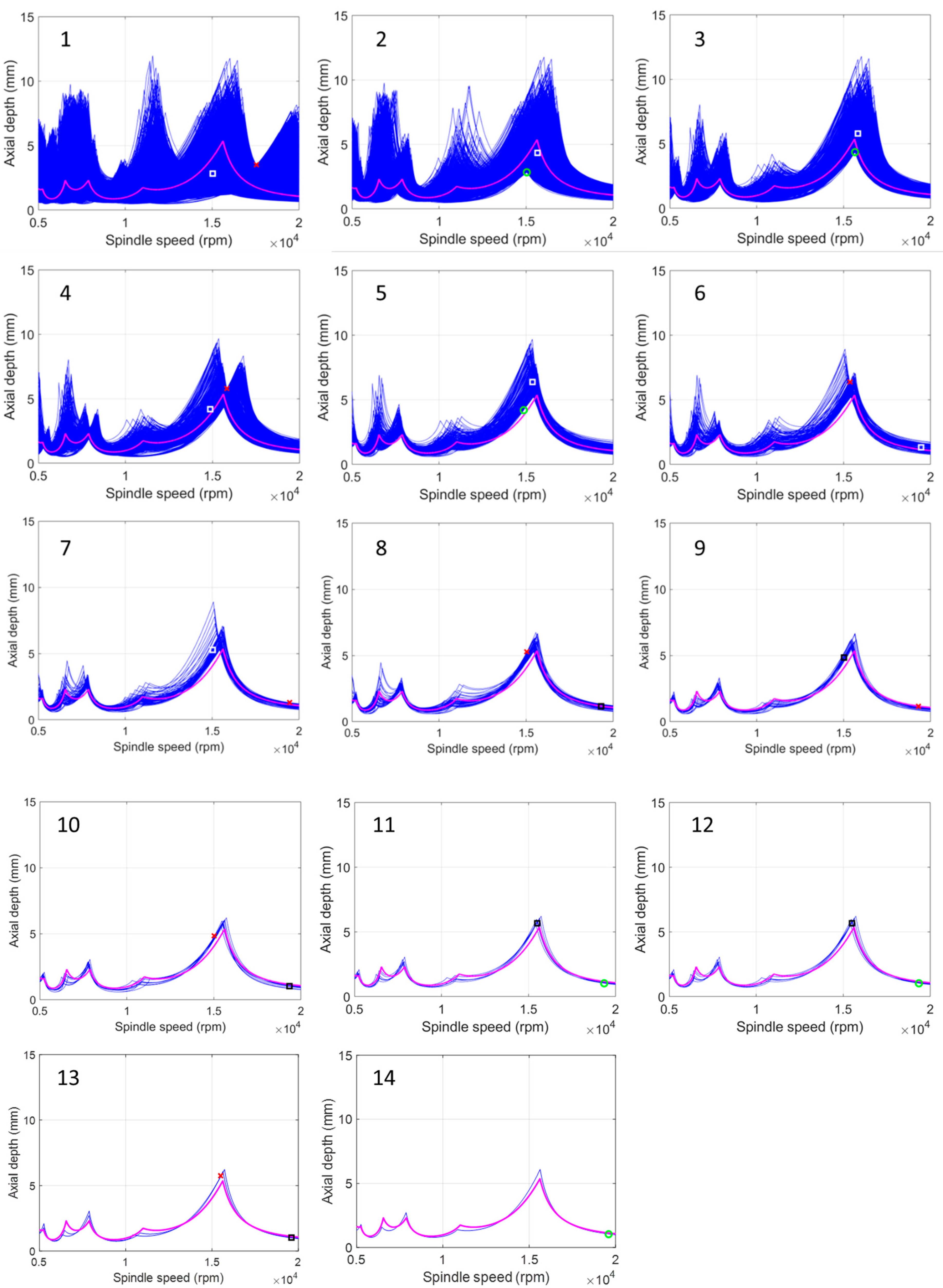
The sample portioning progression over all 14 tests is summarized in Figure 13. It is seen how the limited test results quickly refine the initial stability map distribution. The final map (blue) in panel 14 closely resembles the stability map (magenta) determined using the true values from Table 1. The final values of the stability map input parameters are listed in Table 4. A comparison to the true values is provided.
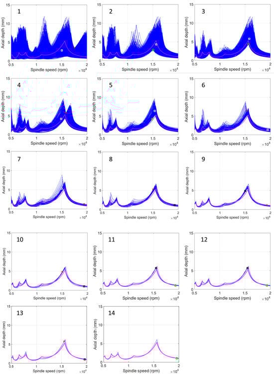
Figure 13.
Sample partitioning results for each test. The remaining maps after each test are shown where the green circle or red × indicates if the test was stable or unstable. The next test point is identified by a square (white or black to provide the best visibility). The numerals 1–14 indicate the test number.
Table 4.
Comparison of stability model inputs after sample partitioning (14 tests) and the true values.
3. Discussion
As seen in Figure 13, the sample partitioning approach effectively reduces the initial 1 × 10⁴ stability maps to a single sample using only 14 tests. Furthermore, the remaining map accurately represents the map obtained from the true model input values. In practice, however, all 14 tests may not be required. The user could elect to discontinue testing at any point using an appropriate stopping criterion. The criterion could be based on the remaining number of samples, changes to the distribution, or test cost, for example. In an ad hoc sense, a review of Figure 13 suggests that test 8 or test 9 could serve as a stopping point since the basic shape of the stability boundary has been identified.
A second observation is that the chatter frequency-based spindle speed selection enabled the domain to be explored and the uncertainty to be reduced. For the case study, the two-mode system caused the chatter frequency to vary between spindle speeds near 15,000 rpm and 19,000 rpm (see Table 2 and Figure 13). The presence of the two modes did not limit the algorithm efficiency.
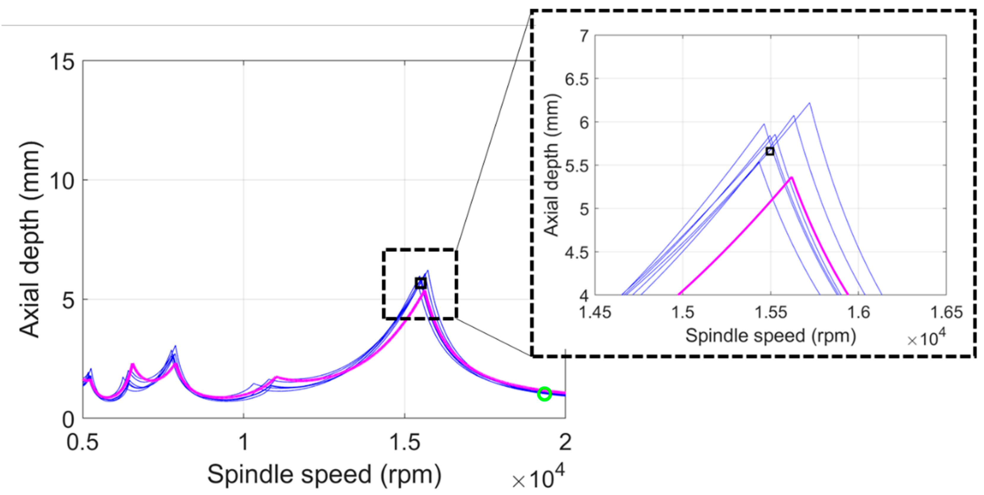
An interesting result was obtained for test 12 as shown in Figure 14. Although the selected test point exceeded the stability boundary defined by the true stability model input parameters, the test point was stable as determined by time domain simulation. This highlights that approximations are applied to obtain the time-invariant, radial-immersion-dependent milling model [6]. Although the model is generally accurate, discrepancies with tests may occur. The sample partitioning therefore serves to select those stability maps that best agree with the test results, not necessarily those that are generated from input parameters that best match the true values. This is emphasized by the results in Table 4, where disagreement between the final and true stability model inputs is observed, but the final stability map provides good agreement with both the test results and the stability map obtained from the true input values.
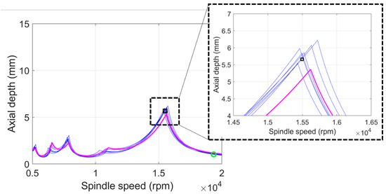
Figure 14.
Point 12 from Table 2 is identified by a black square. Although the result is predicted to be unstable using the stability map predicted from the true model inputs (magenta), it was observed to be stable in the time domain simulation, which provided the test result for this study.
After testing is concluded, the remaining stability maps represent the model for parameter selection. If multiple maps are retained (e.g., 39 samples would remain if testing was discontinued after test 8), then multiple values for each model parameter would remain. The mean values of the modal parameters and cutting force model coefficients at each spindle speed could be calculated, for example, and then used to define the stability map. The final milling parameters would then be based on the user’s risk preference. Most likely, combinations of {spindle speed, axial depth} at the stability boundary would not be selected since it is understood that uncertainty remains, even though it has been reduced by the testing and sample partitioning. It is important to note that the stability map input values identified by testing and sample partitioning can be applied to other milling conditions. For example, the milling direction could be switched from down- to up-milling and the radial depth could be changed. In this way, the method is generalizable to other milling conditions.
To evaluate the parameters from Table 4, the time domain simulation results are compared for up milling with a 5 mm radial depth of cut and 0.15 mm feed per tooth. Recall that the model was developed using a 3 mm radial depth of cut for down milling with a 0.1 mm feed per tooth. To choose the {spindle speed, axial depth} combinations for testing, the stability map was calculated using the frequency domain model [6] and post-partitioning input values from Table 4. Tests were then performed at the spindle speed corresponding to the maximum allowable axial depth from the predicted stability map.
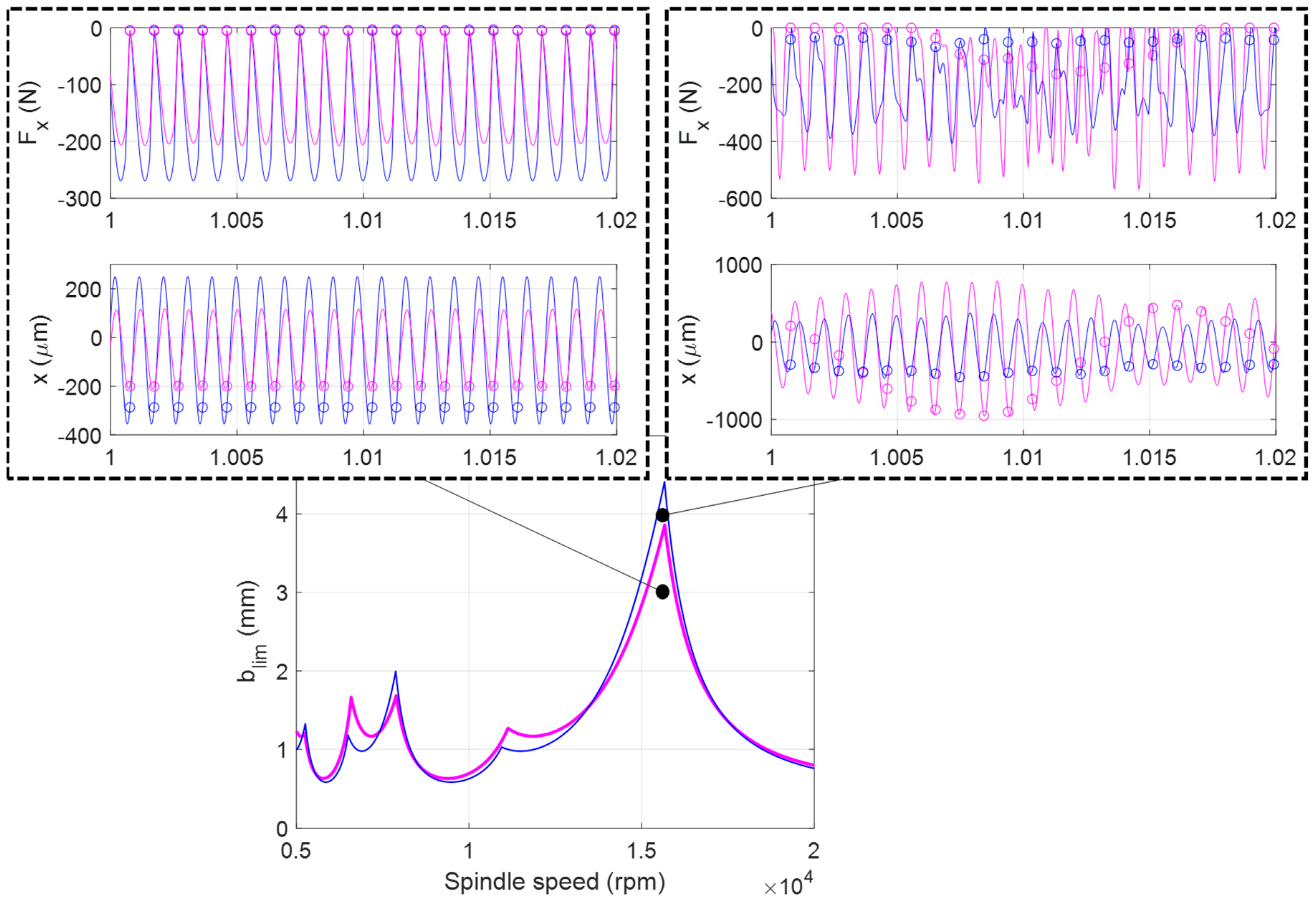
A comparison of the results using the true and post-partitioning values is shown in Figure 15, where the test spindle speed was 15,663 rpm. The axial depths were 3 mm and 4 mm. The stability map for the true values (magenta) predicts the 3 mm axial depth to be stable and the 4 mm axial depth to the unstable. The post-partitioning stability map (blue) predicts both axial depths to be stable; the local peak in this map is located at {15,663 rpm, 4.41 mm}. The left inset shows that the 3 mm axial depth is stable for both parameters set. Due to the larger cutting force coefficients for the post-partitioning results, the corresponding x-direction force, Fx, is larger (blue). Because the force is larger, the x-direction vibration response (blue) is also larger. The circles represent the once-per-tooth samples. Because they repeat from one tooth passage to the next, forced vibration is present and the cutting conditions are stable [25].
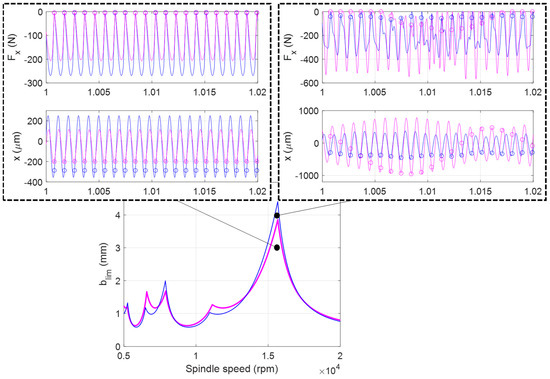
Figure 15.
Comparison of results using the true (magenta) and post-partitioning (blue) values.
The right inset shows that the 4 mm axial depth is unstable for both parameters set. Due to the larger stiffness values for the post-partitioning results, the behavior is only marginally unstable (blue). This is demonstrated by the variation in the force profile from one tooth to the next, but only a small variation in the once-per-tooth samples. The behavior for true values exhibits fully developed chatter (magenta).
4. Conclusions
This paper described a milling modeling approach that implemented sample partitioning to retain or reject samples from an initial distribution of stability maps using milling test results. Because the stability model input parameters are also partitioned using the test results, their uncertainty is reduced using the test results and the milling stability model accuracy is increased. In a case study, the stability maps were calculated from distributions of uncertain: (1) modal parameters that represent the tool tip frequency response functions, and (2) cutting force model coefficients. Test points were selected based on the previous test result. If the previous test was stable, the combination of spindle speed and mean axial depth from the remaining samples that provides the high material removal rate was selected. If the previous test was unstable, the spindle speed for the next test was calculated using the chatter frequency, where the tooth passing frequency was set equal to the chatter frequency. The mean axial depth at that spindle speed was then selected to fully define the test point.
A case study validated the approach. For a selected milling system, defined by a two-mode symmetric frequency response function and mechanistic cutting force model, initial uniform distributions for the stability model input parameters were reduced from 1 × 10⁴ samples to a single final sample in only 14 tests. The remaining stability map provided good agreement to the stability map produced from the true model input values. A discussion was provided that explored stopping criteria, multiple chatter frequencies, disagreement between the time domain simulation (used for testing here) and the frequency domain stability model, and final milling parameter selection given the reduced uncertainty model after testing, including generalizability.
Funding
The author gratefully acknowledges support from MxD (Manufacturing x Digital) and the NSF Engineering Research Center for Hybrid Autonomous Manufacturing Moving from Evolution to Revolution (ERC-HAMMER) under Award Number EEC-2133630.
Data availability statement
Data are contained within the article.
Conflicts of Interest
The authors declare that they have no known competing financial interests or personal relationships that could have appeared to influence the work reported in this paper.
References
- Altintas, Y.; Stepan, G.; Budak, E.; Schmitz, T.; Kilic, Z.M. Chatter stability of machining operations. ASME J. Manuf. Sci. Eng. 2020, 142, 110801. [Google Scholar] [CrossRef]
- Ewins, D.J. Modal Testing: Theory, Practice and Application; John Wiley & Sons: Hoboken, NJ, USA, 2009. [Google Scholar]
- Schmitz, T.; Smith, K.S. Machining Dynamics: Frequency Response to Improved Productivity, 2nd ed.; Springer: Berlin/Heidelberg, Germany, 2019. [Google Scholar]
- Kim, H.S.; Schmitz, T.L. Bivariate uncertainty analysis for impact testing. Meas. Sci. Technol. 2007, 18, 3565. [Google Scholar] [CrossRef]
- Altintas, Y. Manufacturing Automation: Metal Cutting Mechanics, Machine Tool Vibrations, and CNC Design; Cambridge University Press: Cambridge, UK, 2000. [Google Scholar]
- Altintas, Y.; Budak, E. Analytical prediction of stability lobes in milling. CIRP Ann. 1995, 44, 357–362. [Google Scholar] [CrossRef]
- Campomanes, M.L.; Altintas, Y. An improved time domain simulation for dynamic milling at small radial immersions. J. Manuf. Sci. Eng. 2003, 125, 416–422. [Google Scholar] [CrossRef]
- Denkena, B.; Grabowski, R.; Krödel, A.; Ellersiek, L. Time-domain simulation of milling processes including process damping. CIRP J. Manuf. Sci. Technol. 2020, 30, 149–156. [Google Scholar] [CrossRef]
- Altintas, Y.; Stépán, G.; Merdol, D.; Dombóvári, Z. Chatter stability of milling in frequency and discrete time domain. CIRP J. Manuf. Sci. Technol. 2008, 1, 35–44. [Google Scholar] [CrossRef]
- Kahraman, M.F.; Bilge, H.; Öztürk, S. Uncertainty analysis of milling parameters using Monte Carlo simulation, the Taguchi optimization method and data-driven modeling. Mater. Test. 2019, 61, 477–483. [Google Scholar] [CrossRef]
- Gul, E.; Joseph, V.R.; Yan, H.; Melkote, S.N. Uncertainty quantification of machining simulations using an in situ emulator. J. Qual. Technol. 2018, 50, 253–261. [Google Scholar] [CrossRef]
- Madić, M.; Radovanović, M. Possibilities of using Monte Carlo method for solving machining optimization problems. Facta Univ. Ser. Mech. Eng. 2014, 12, 27–36. [Google Scholar]
- Delio, T.; Tlusty, J.; Smith, S. Use of audio signals for chatter detection and control. ASME J. Eng. Ind. 1992, 114, 146–157. [Google Scholar] [CrossRef]
- Maamar, A.; Le, T.P.; Gagnol, V.; Sabourin, L. Modal identification of a machine tool structure during machining operations. Int. J. Adv. Manuf. Technol. 2019, 102, 253–264. [Google Scholar] [CrossRef]
- Gagnol, V.; Le, T.P.; Ray, P. Modal identification of spindle-tool unit in high-speed machining. Mech. Syst. Signal Process. 2011, 25, 2388–2398. [Google Scholar] [CrossRef]
- Zaghbani, I.; Songmene, V. Estimation of machine-tool dynamic parameters during machining operation through operational modal analysis. Int. J. Mach. Tools Manuf. 2009, 49, 947–957. [Google Scholar] [CrossRef]
- Wang, M.; Gao, L.; Zheng, Y. An examination of the fundamental mechanics of cutting force coefficients. Int. J. Mach. Tools Manuf. 2014, 78, 1–7. [Google Scholar] [CrossRef]
- Altintas, Y.; Eynian, M.; Onozuka, H. Identification of dynamic cutting force coefficients and chatter stability with process damping. CIRP Ann. 2008, 57, 371–374. [Google Scholar] [CrossRef]
- Campatelli, G.; Scippa, A. Prediction of milling cutting force coefficients for Aluminum 6082-T4. Procedia CIRP 2012, 1, 563–568. [Google Scholar] [CrossRef]
- Popović, M.; Tanović, L.; Ehmann, K.F. Cutting forces prediction: The experimental identification of orthogonal cutting coefficients. FME Trans. 2017, 45, 459–467. [Google Scholar] [CrossRef]
- von Hahn, T.; Mechefske, C.K. Machine Learning in CNC Machining: Best Practices. Machines 2022, 10, 1233. [Google Scholar] [CrossRef]
- Insperger, T.; Stépán, G.; Bayly, P.V.; Mann, B.P. Multiple chatter frequencies in milling processes. J. Sound Vib. 2003, 262, 333–345. [Google Scholar] [CrossRef]
- Cramér, H. Random Variables and Probability Distributions; Cambridge University Press: Cambridge, UK, 2004. [Google Scholar]
- Tekeli, A.; Budak, E. Maximization of chatter-free material removal rate in end milling using analytical methods. Mach. Sci. Technol. 2005, 9, 147–167. [Google Scholar] [CrossRef]
- Honeycutt, A.; Schmitz, T.L. Milling stability interrogation by subharmonic sampling. J. Manuf. Sci. Eng. 2017, 139, 041009. [Google Scholar] [CrossRef]


Disclaimer/Publisher’s Note: The statements, opinions and data contained in all publications are solely those of the individual author(s) and contributor(s) and not of MDPI and/or the editor(s). MDPI and/or the editor(s) disclaim responsibility for any injury to people or property resulting from any ideas, methods, instructions or products referred to in the content. |
© 2024 by the author. Licensee MDPI, Basel, Switzerland. This article is an open access article distributed under the terms and conditions of the Creative Commons Attribution (CC BY) license (https://creativecommons.org/licenses/by/4.0/).