Material Parameter Identification for a Stress-State-Dependent Ductile Damage and Failure Model Applied to Clinch Joining

Abstract

Similar to bulk metal forming, clinch joining is characterised by large plastic deformations and a variety of different 3D stress states, including severe compression. However, inherent to plastic forming is the nucleation and growth of defects, whose detrimental effects on the material behaviour can be described by continuum damage models and eventually lead to material failure. As the damage evolution strongly depends on the stress state, a stress-state-dependent model is utilised to correctly track the accumulation. To formulate and parameterise this model, besides classical experiments, so-called modified punch tests are also integrated herein to enhance the calibration of the failure model by capturing a larger range of stress states and metal-forming-specific loading conditions. Moreover, when highly ductile materials are considered, such as the dual-phase steel HCT590X and the aluminium alloy EN AW-6014 T4 investigated here, strong necking and localisation might occur prior to fracture. This can alter the stress state and affect the actual strain at failure. This influence is captured by coupling plasticity and damage to incorporate the damage-induced softening effect. Its relative importance is shown by conducting inverse parameter identifications to determine damage and failure parameters for both mentioned ductile metals based on up to 12 different experiments.

1. Introduction

Ductile damage and failure modelling remains a challenge, especially for bulk metal forming and related processes [1]. These are typically characterised by large plastic strains, complex loading paths, and all kinds of stress states, including severe compression. These various loading situations make it particularly difficult to calibrate damage and failure models.

Clinching belongs to the mechanical joining methods and assembles different sheet metal blanks by pure cold forming [2]. It is thus characterised similarly to bulk metal forming by high plastic strains of up to 300% and strong compressive loading. During joining, a sufficient interlock must be formed to obtain the desired joint strength, which involves shearing and tensile loading, thereby increasing the diversity of the stress states. As the joint strength solely relies on the sheet material and its directed deformation during the joining process, accurate and predictive material models are required [3].

During forming, plastic incompressibility can cause new microscopic voids, pores, and defects to nucleate or existing flaws to grow, link, or coalesce (compare, for instance, the reviews on experimental observations [4] with those on the evolution mechanisms of microdefects [5]). These processes can degrade the material, which is herein phenomenologically modelled as ductile damage. Damage evolves hidden inside the material and eventually leads to macroscopic material fracture. Experiments have led to the observation that materials exhibit different failure mechanisms and strains at fracture under different stress states [6,7,8]. As the material inherently passes through a variety of stress states during the considered forming process, a stress-state-dependent damage and failure model is applied [9]. However, to calibrate such a widely applicable material model for the relevant range of stress states, various experiments probing different stress states and loading paths are required. Classical experiments using smooth and notched tensile and shear specimens often span only a certain stress spectrum. Therefore, compressive loading typically misses, as well as the for metal forming typical transition from strong compression to shear/tension, which eventually leads to fracture [1,10]. Based on this, punch tests have been developed [11] that can cover a wide range of stress states, including compression, and bring the loading conditions closer to the targeted application. Systematic changes in the punch and die shape enable an adjustment of the stress state up to failure. However, due to the closed setup, no direct observation of the process and, most interestingly, the fracture initiation location, is possible. Moreover, due to the axisymmetric setup, typically only a limited range of stress states can be reached. To resolve these limitations, so-called modified punch tests were developed in [12], which consist of a half-setup where the classical punch test is cut in half so that only a 180° section is probed. This cut setup allows for direct visual access to the cross-section where fracture initiation is expected to occur. Hence, the process, as well as failure evolution, can be observed in situ with digital image correlation (DIC). This provides deeper insight and more flexibility regarding the experimental setup and the achievable stress states [13,14].

However, an experimentally driven determination of the failure locus is faced with a multitude of challenges. These can further lead to conflicting results and interpretations. The identification of the fracture initiation location, for instance, is challenging, as strain localisation might obscure or shift the actual site. For instance, the crack in notched shear specimens might not initiate at the initial notch location, as one would intuitively assume, but a new “notch” can form due to the ductility of the material [15]. Especially under compression, complex mechanisms are present, and failure might initiate at partially hidden irregularities [16]. Such circumstances are common to many investigated specimens and can strongly alter the actual stress state and hence the calibration. Large plastic deformations, rotations, and necking can further alter the stress state along the loading path. Thus, a uniaxial tensile test with a theoretical stress triaxiality of $1/3$ will eventually fail after necking and strain localisation at a much higher triaxiality of more than $0.7$ for ductile materials. Even more critical are shear specimens, where a theoretical triaxiality of 0 might be aimed for, but failure can eventually occur closer to biaxial tension, as studied in [17]. In [18], the influence of the chosen characterisation experiments on the resulting failure locus was investigated. The results were shown to be non-unique and possibly also dependent on the non-coaxiality of the loading path. Another influencing factor may be the stress-softening effect caused by the evolution of ductile damage. Even though various experimental methods are available for measuring this softening effect (see the comparison in [19]), it remains challenging. Thus, it is difficult to reason about its actual influence. Nevertheless, it is generally agreed that damage mechanisms eventually lead to fracture, even if they occur very late during loading, as observed in [20]. In any case, as damage-induced softening leads to strong strain localisation, especially for the considered ductile metals, experimental measurement of strains up to fracture is challenging and strongly constrained by the gauge size [21]. Especially for shear loading, the experimentally determined failure strain inside the shear band can be underestimated by a factor of more than 2 [22,23].

This short overview of some challenges emphasises the complexity of ductile damage and failure evolution. To investigate the influence of damage-induced changes in the stress state, a fully coupled plasticity–damage model is used, which is briefly reiterated in Section 2.1. Inverse parameter identification using finite-element simulations is performed, and the results of up to 12 experiments, including classical tests, as well as punch and modified punch tests, are presented. This further helps minimise a priori assumptions, for instance, on the crack initiation location.

2. Materials and Methods

The material model is briefly reiterated in Section 2.1 to introduce the relevant material parameters that need to be identified. Section 2.2 outlines the experimental setups, which include classical characterisation experiments, as well as standard and modified punch tests. Subsequently, in Section 2.3, the corresponding simulation setups are sketched to reconstruct the experiments. The experimental results together with the simulation models are then input and processed in the parameter identification. The general procedure is outlined in Section 2.4 and then conducted in Section 3.

2.1. Constitutive Model and Material Parameters

The material model is a hyperelastic-based finite plasticity model suitable for large plastic strains. It is fully coupled to a stress-state-dependent ductile damage model detailed in [9]. This constitutive model is briefly summarised here to introduce the material parameters listed in

Table 1. Summary of relevant material parameters to be identified. The failure model is a combination of the Cockcroft–Latham–Oh (CLO) and the Hosford–Coulomb (HC) failure models.

Symbol	Description	Identification	Unit
Elasticity
E	Young’s modulus	measurement	MPa
$\nu$	Poisson’s ratio	literature	–
Plasticity
${\sigma }_y$	initial yield stress	direct fit to experiment	MPa
K	hardening modulus	direct fit to experiment	MPa
$n_{\mathrm{p},K}$	power-law exponent	direct fit to experiment	–
$\Delta {\sigma }_{y,\infty }$	yield-stress increment	direct fit to experiment	MPa
$\omega$	hardening saturation	direct fit to experiment	–
$n_{\mathrm{p},\omega }$	saturation exponent	direct fit to experiment	–
Damage
$\eta ={\eta }_{\mathrm{vol}}={\eta }_{\mathrm{dev}}={\eta }_{\mathrm{p}}$	damage saturation	assumed value, 1	–
${\eta }_{\mathrm{f}}$	damage saturation (failure)	deduction from experiments	–
${\mathcal{F}}^{\mathrm{crit}}$	critical failure indicator	deduction from experiments	–
Failure
$n_{\mathrm{d}}$	failure exponent	assumed value, 1	–
$b_{\mathrm{CLO}}$	failure strain at shear for CLO-model	inverse identification	–
$a_{\mathrm{f}}$	Hosford–Coulomb parameter a	inverse identification	–
$b_{\mathrm{f}}$	Hosford–Coulomb parameter b	inverse identification	–
$c_{\mathrm{f}}$	Hosford–Coulomb parameter c	inverse identification	–
$n_{\mathrm{f}}$	Hosford–Coulomb parameter n	literature	–

that are identified herein.

The elastic response of the model is governed by the Young’s modulus E and the Poisson’s ratio $\nu$ and is limited to small elastic strains, which is suitable for metal forming. Isotropic von Mises plasticity is considered with plastic hardening described by an analytical flow stress equation as follows:

$${\sigma }_{\mathrm{flow}}\left(\alpha \right)={\sigma }_y+K{\alpha }^{n_{\mathrm{p},K}}+\Delta {\sigma }_{y,\infty }\left[1-exp(-\omega {\alpha }^{n_{\mathrm{p},\omega }})\right]$$

(1)

with the initial yield stress ${\sigma }_y$ and the plastic-hardening variable $\alpha$, similar to the accumulated plastic strain. Thereby, a power-law plastic hardening is chosen with the hardening modulus K and power-law exponent $n_{\mathrm{p},K}$, and combined with exponential hardening with the exponential yield-stress increment $\Delta {\sigma }_{y,\infty }$, the saturation parameter $\omega$, and the additional saturation exponent $n_{\mathrm{p},\omega }$. This renders non-linear isotropic hardening with six material parameters for plasticity.

Material failure is modelled by a stress-state-dependent failure surface. The stress-state dependency is governed by the stress triaxiality $\mathcal{X}$ and the Lode angle parameter $\overline{\mathcal{L}}$, defined based on the Cauchy stress tensor $\sigma$ as

$$\begin{array}{cc}\hfill \mathcal{X}& \equiv {\displaystyle \frac{{\sigma }^{\mathrm{vol}}}{{\sigma }_{\mathrm{vM}}}}\mathrm{with}{\sigma }^{\mathrm{vol}}\equiv {\displaystyle \frac{1}{3}}\mathrm{tr}\sigma ,{\sigma }_{\mathrm{vM}}\equiv \sqrt{{\displaystyle \frac{3}{2}}}∥{\sigma }^{\mathrm{dev}}∥\hfill \end{array}$$

(2)

$$\begin{array}{cc}\hfill & \mathrm{with}{\sigma }^{\mathrm{dev}}\equiv \sigma -{\sigma }^{\mathrm{vol}}\mathit{I}\mathrm{and}∥(•)∥\equiv \sqrt{\sum _{i=1}^3\sum _{j=1}^3{\left[{(•)}_{ij}\right]}^2}\hfill \end{array}$$

(3)

$$\begin{array}{cc}\hfill \overline{\mathcal{L}}& =1-{\displaystyle \frac{2}{\pi }}arccos\left(\mathcal{L}\right)\begin{array}{c}\hfill \in \left[-1,1\right]\end{array}\mathrm{with}\mathcal{L}\equiv {\displaystyle \frac{27}{2}}{\displaystyle \frac{det\left({\sigma }^{\mathrm{dev}}\right)}{{\left[{\sigma }_{\mathrm{vM}}\right]}^3}}\begin{array}{c}\hfill \in \left[-1,1\right]\end{array}\hfill \end{array}$$

(4)

For the description of the failure surface, which provides the strain at material failure ${\alpha }^{\mathrm{f}}(\mathcal{X},\overline{\mathcal{L}})$ as a function of the stress state, a combination of the Cockcroft–Latham–Oh [24] and the Hosford–Coulomb [25] failure models is used.

Cockcroft–Latham–Oh (CLO) failure model:

$$\begin{array}{c}\hfill {\alpha }_{\mathrm{CLO}}^{\mathrm{f}}(\mathcal{X},\overline{\mathcal{L}})\equiv {\displaystyle \frac{\sqrt{3}/3b_{\mathrm{CLO}}}{{\left[\mathcal{X}+l_1\right]}^{+}}}\mathrm{with}{\left[(•)\right]}^{+}\equiv {\displaystyle \frac{1}{2}}\left[(•)+\left|(•)\right|\right]\begin{array}{c}\hfill ,\left|(•)\right|\equiv \sqrt{{\left[(•)\right]}^2}\end{array}\end{array}$$

(5)

Hosford–Coulomb (HC) failure model:

$$\begin{array}{c}\hfill {\alpha }_{\mathrm{HC}}^{\mathrm{f}}(\mathcal{X},\overline{\mathcal{L}})\equiv b_{\mathrm{f}}{\left[{\displaystyle \frac{1+c_{\mathrm{f}}}{g_{\mathrm{f}}(\mathcal{X},\overline{\mathcal{L}})}}\right]}^{1/n_{\mathrm{f}}}\end{array}$$

(6)

$$\begin{array}{c}\hfill \mathrm{with}{g}_{\mathrm{f}}(\mathcal{X},\overline{\mathcal{L}})\equiv {\left[{\displaystyle \frac{1}{2}}\left[{\left[l_1-l_2\right]}^{a_{\mathrm{f}}}+{\left[l_2-l_3\right]}^{a_{\mathrm{f}}}+{\left[l_1-l_3\right]}^{a_{\mathrm{f}}}\right]\right]}^{1/a_{\mathrm{f}}}+c_{\mathrm{f}}\left[2\mathcal{X}+l_1+l_3\right]\end{array}$$

(7)

$$\begin{array}{cc}\hfill \mathrm{with}{l}_1& \equiv {\displaystyle \frac{2}{3}}cos\left({\displaystyle \frac{\pi }{6}}\left[1-\overline{\mathcal{L}}\right]\right)\hfill \\ \hfill l_2& \equiv {\displaystyle \frac{2}{3}}cos\left({\displaystyle \frac{\pi }{6}}\left[3+\overline{\mathcal{L}}\right]\right)\hfill \\ \hfill l_3& \equiv -{\displaystyle \frac{2}{3}}cos\left({\displaystyle \frac{\pi }{6}}\left[1+\overline{\mathcal{L}}\right]\right)\hfill \end{array}$$

(8)

Combined Cockcroft–Latham–Oh + Hosford–Coulomb failure model:

$${\alpha }_{\mathrm{CLO}+\mathrm{HC}}^{\mathrm{f}}(\mathcal{X},\overline{\mathcal{L}})=\left\{\begin{array}{cc}{\alpha }_{\mathrm{CLO}}^{\mathrm{f}}(\mathcal{X},\overline{\mathcal{L}})\hfill & \mathrm{for}\mathcal{X}\le 0\hfill \\ \left[1-3\mathcal{X}\right]{\alpha }_{\mathrm{CLO}}^{\mathrm{f}}(\mathcal{X},\overline{\mathcal{L}})+\left[1-\left[1-3\mathcal{X}\right]\right]{\alpha }_{\mathrm{HC}}^{\mathrm{f}}(\mathcal{X},\overline{\mathcal{L}})\hfill & \mathrm{for}0<\mathcal{X}<1/3\hfill \\ {\alpha }_{\mathrm{HC}}^{\mathrm{f}}(\mathcal{X},\overline{\mathcal{L}})\hfill & \mathrm{for}\mathcal{X}\ge 1/3\hfill \end{array}\right.$$

(9)

This leads to five parameters for the combined failure model: $b_{\mathrm{CLO}}$ describes the failure strain for pure shear ($\mathcal{X}=0,\overline{\mathcal{L}}=0$); $b_{\mathrm{f}}$ is the failure strain at uniaxial tension ($\mathcal{X}=1/3,\overline{\mathcal{L}}=1$); $a_{\mathrm{f}}\le 2$ describes the depth of the Lode valley, being deeper for smaller values, where the upper bound value of 2 renders no valley; and $c_{\mathrm{f}}$ and $n_{\mathrm{f}}$ relate to the decrease in the failure strain with increasing triaxiality. The combined failure strain ${\alpha }_{\mathrm{CLO}+\mathrm{HC}}^{\mathrm{f}}(\mathcal{X},\overline{\mathcal{L}})$ governs the evolution of a failure indicator $\mathcal{F}$, as defined in Equation (10), which is driven by plasticity and can grow nonlinearly depending on a failure exponent $n_{\mathrm{d}}$. Therein, also the damage-driving variable ${\alpha }^{\mathrm{d}}$ is equipped with the Cockcroft–Latham–Oh cut-off triaxiality ${\mathcal{X}}_{\mathrm{cut}-\mathrm{off}}=-l_1$ below which ${\alpha }^{\mathrm{d}}$ does not accumulate [9]. Once $\mathcal{F}$ reaches a value of 1, material fracture is initiated.

$$\mathcal{F}={\int }_0^{{\alpha }_{*}^{\mathrm{f}}}{\displaystyle \frac{n_{\mathrm{d}}{\left[{\alpha }^{\mathrm{d}}\right]}^{n_{\mathrm{d}}-1}}{{\left[{\alpha }^{\mathrm{f}}(\mathcal{X},\overline{\mathcal{L}})\right]}^{n_{\mathrm{d}}}}}\mathrm{d}{\alpha }^{\mathrm{d}}\mathrm{with}\dot{{\alpha }^{\mathrm{d}}}=\left\{\begin{array}{cc}\sqrt{{\displaystyle \frac{2}{3}}}\dot{{\gamma }^{\mathrm{p}}},\hfill & \mathrm{if}\mathcal{X}>{\mathcal{X}}_{\mathrm{cut}-\mathrm{off}}=-l_1\hfill \\ 0,\hfill & \mathrm{otherwise}\hfill \end{array}\right.$$

(10)

The softening effect of ductile damage on the material response is introduced by the damage variable d. d is set up to degrade the elastic material parameters and the flow stress by the common degradation function $\left[1-\eta d\right]$. For simplicity, elasticity and plasticity are degraded with an identical damage saturation value $\eta$. Ductile damage is determined from the failure indicator using Equation (11). However, as the failure indicator initially grows much faster than the material actually degrades, a piecewise linear mapping is proposed.

$$\begin{array}{c}\hfill d=\left\{\begin{array}{cc}{\eta }_{\mathrm{f}}\mathcal{F},\hfill & \mathrm{if}\mathcal{F}\le {\mathcal{F}}^{\mathrm{crit}}\hfill \\ {\displaystyle \frac{{\displaystyle 1-{\eta }_{\mathrm{f}}{\mathcal{F}}^{\mathrm{crit}}}}{{\displaystyle 1-{\mathcal{F}}^{\mathrm{crit}}}}}\mathcal{F}-{\displaystyle \frac{{\displaystyle {\mathcal{F}}^{\mathrm{crit}}\left[1-{\eta }_{\mathrm{f}}\right]}}{{\displaystyle 1-{\mathcal{F}}^{\mathrm{crit}}}}},\hfill & \mathrm{otherwise}\hfill \end{array}\right.\end{array}$$

(11)

The damage-failure mapping is thus related to two material parameters: the initial slope governed by the saturation parameter ${\eta }_{\mathrm{f}}$ and the critical failure indicator ${\mathcal{F}}^{\mathrm{crit}}$ describing the transition point from the slow to the accelerated damage growth.

Table 1 summarises all relevant material parameters and how they are identified. Young’s modulus, for instance, is directly measured with a special experimental setup, as explained later in Section 2.4. Plasticity parameters that describe the flow stress are directly fitted to experimentally determined flow curves. In the end, only four failure parameters need to be identified by inverse parameter identification.

The material model is implemented as a user-defined material into the commercial finite-element software LS-DYNA, version R13. Further details on this constitutive model, its algorithmic implementation, and regularisation can be found in [9]. Here, gradient enhancement is not applied to introduce a length scale and regularise stress softening. This reduces the computational effort for inverse parameter identification by avoiding the need for very small element sizes, which are necessary if a realistic length scale is chosen, as exemplarily shown in [9].

2.2. Experimental Setups

The investigations were conducted on a dual-phase steel HCT590X and an aluminium alloy EN AW-6014 in the T4 temper. The chemical composition and mechanical properties of the investigated materials according to the manufacturers’ datasheets are listed in

Table 2. Chemical compositions and mechanical properties of investigated HCT590X [26] and EN AW-6014 T4 [27].

	HCT590X (wt %)			EN AW-6014 T4 (wt %)
Chemical composition		Min.	Max.		Min.	Max.
	C		0.15	Si		0.60
	Si		0.75	Fe		0.35
	Mn		2.5	Cu		0.25
	P		0.04	Mn	0.05	0.20
	S		0.015	Mg	0.40	0.80
	Al	0.015	1.5	Cr		0.20
	Cr + Mo		1.4	Zn		0.10
	Nb + Ti		0.15	Ti		0.10
				V		0.10
Physical properties	Yield strength Rp0.2 (MPa)	330–430			≤130
	Ultimate tensile strength Rm (MPa)	590–700			≥175
	Elongation A80 (%)	≥20			≥23

.

For the experimental identification of the failure parameters for a wide range of stress states, several tests were utilised [13]. Classical tests from forming technology can be used, such as tensile, compression, or bulge tests. Moreover, it is common for tensile and punch tests to specifically adapt the specimen or tool geometry to achieve the defined stress states. Recently, a modified punch test has also been developed [12], which is similar in its kinematics to the targeted clinching process and allows for a variation of stress states and optical accessibility of the specimen. Each section concludes with a summary of the significance of the experiment described for parameter identification.

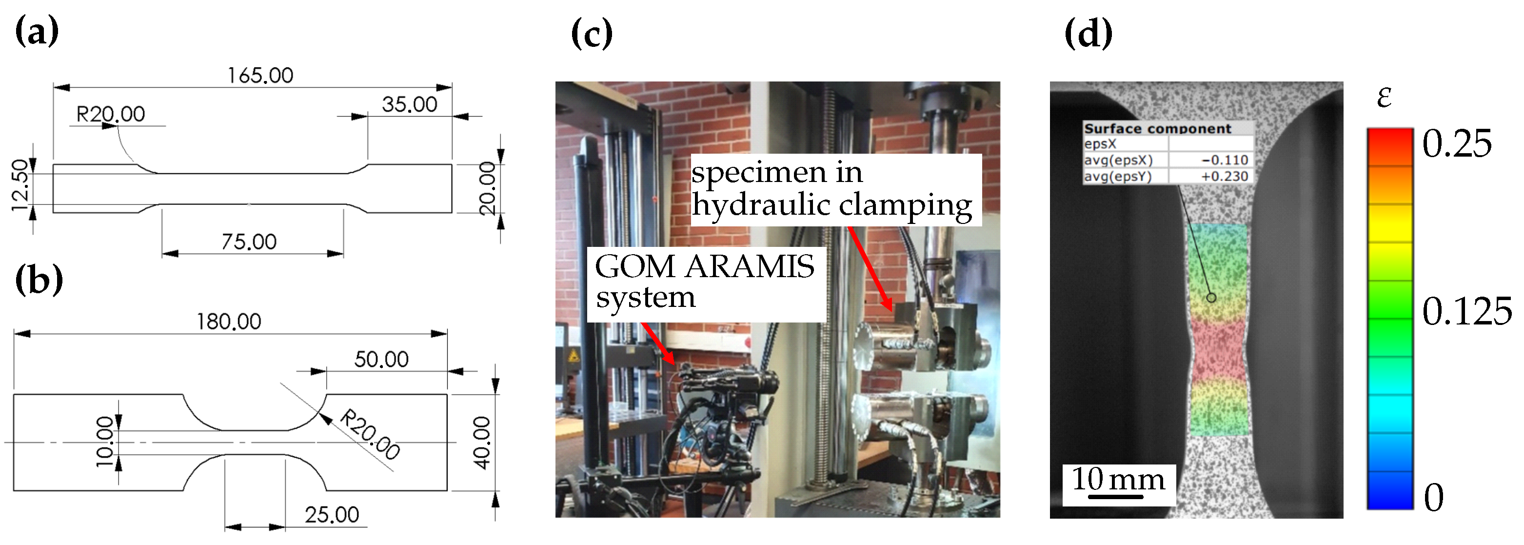
2.2.1. Tensile Tests

According to the ISO 6892-1 standard [28], the tensile test (Figure 1) is one of the most widely applied methods for characterising sheet metal materials. It is characterised by a comparatively simple test procedure and low experimental and time effort [29]. It provides a frictionless and uniaxial stress condition at plastic strains between $0.1$ and $0.8$, depending on the material strength [30]. However, the uniaxial stress condition is only present up to uniform strain. In addition to the conventional tensile test, the strain-hardening behaviour can be investigated at higher strain rates of the materials. For this purpose, further specimen geometries are defined, as shown in [31]. In this study, two different specimen geometries were examined for the tensile tests in order to consider the influence of the specimen geometry. Even though the specimen geometry does not alter the response up to uniform strain, it can affect necking and eventually failure. This paves the way for future incorporation of strain rate effects into the plasticity and damage model utilising the SEP1230 setup in [31]. Tensile specimens were tested according to specimen form H in accordance with DIN 50125 [32] with a gauge length of 50 mm. In addition, specimens were tested according to SEP1230 with a gauge length of 20 mm. The specimen dimensions are shown in Figure 1a,b. The specimens were produced by wire erosion from sheet metal with longitudinal alignment to the rolling direction.

The tensile tests for determining the stress–strain curves of the investigated materials were performed on a Zwick Z100 tensile-compression testing machine, as shown in Figure 1c, with a maximum test load of 100 kN. All tests were performed using a digital image correlation (DIC) system (GOM ARAMIS), as shown in Figure 1d. The tensile tests were performed at a strain rate of 0.001 s⁻¹.

The tensile tests provide an initially uniaxial loading, which is important for the calibration of the flow stress. Further, the necking behaviour can be utilised to verify the flow stress beyond uniform strain. The situation is more difficult concerning the identification of failure parameters for highly ductile materials. The strong necking notably alters the stress states and is further accelerated by coupling plasticity and damage. Therefore, the tensile test mainly captures the failure behaviour at higher and varying triaxialities.

2.2.2. Plane-Strain Tensile Test

To achieve approximately plane-strain states with comparatively high triaxialities, specimens were manufactured and tested according to the dimensions in Figure 2a. This specimen is characterised by a defined notch in the sheet thickness direction. The Z100 tensile-compression testing machine was also used here, and the displacement measurement and strain measurement were realised locally using a GOM ARAMIS system (Figure 2b). The dimensions of the specimens were selected based on [34].

This notched specimen obtains a plane-strain state, which is important for probing the yield surface at different stress states and refining its shape. This plane-strain state with Lode angle parameter $\overline{\mathcal{L}}=0$ is also insightful for failure calibration, as it captures the valley in the failure surface at high triaxialities above $0.6$.

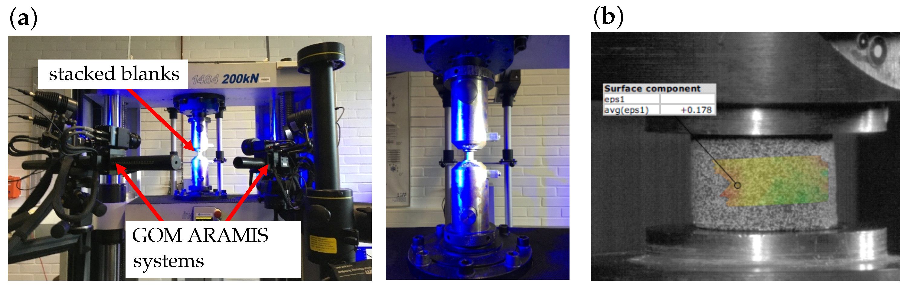
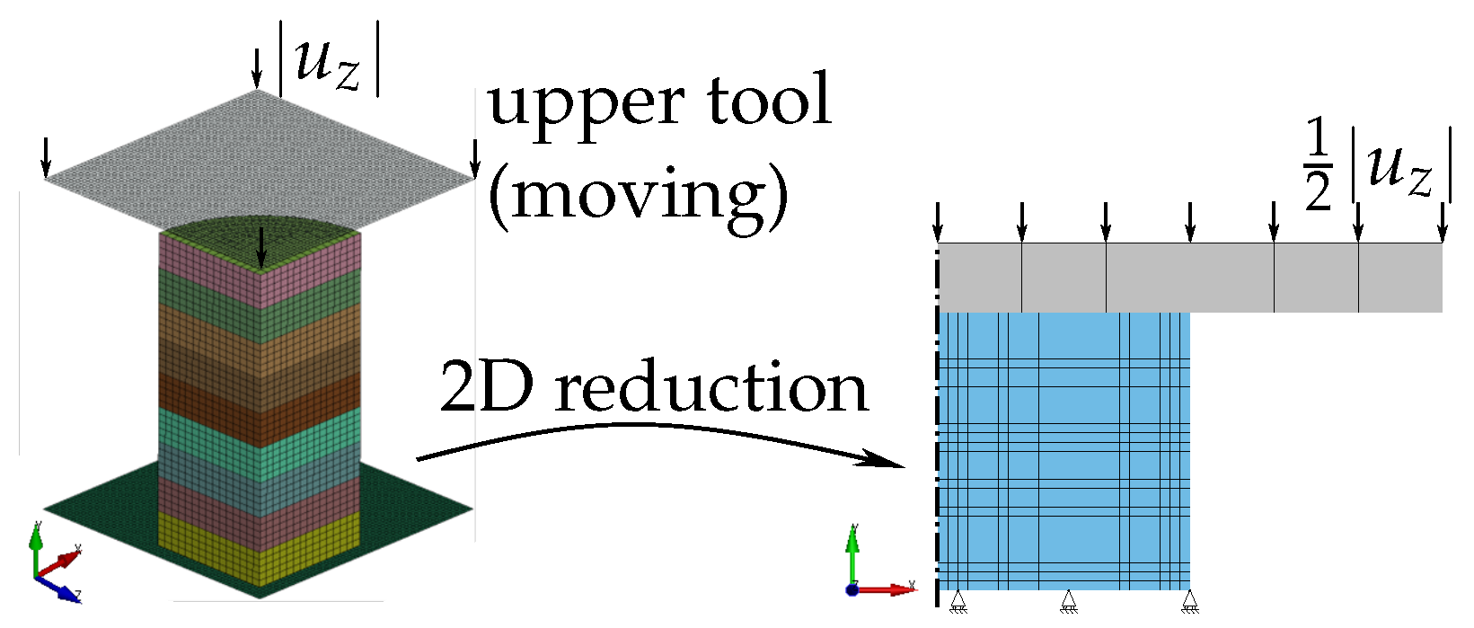
2.2.3. Layer Compression Test

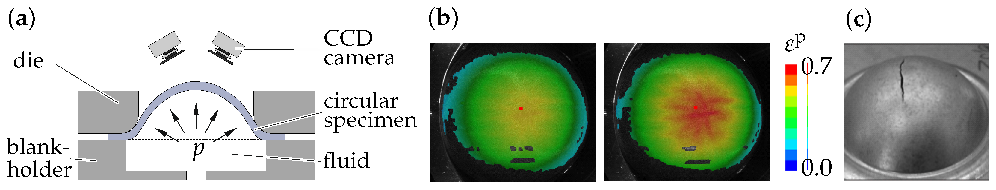
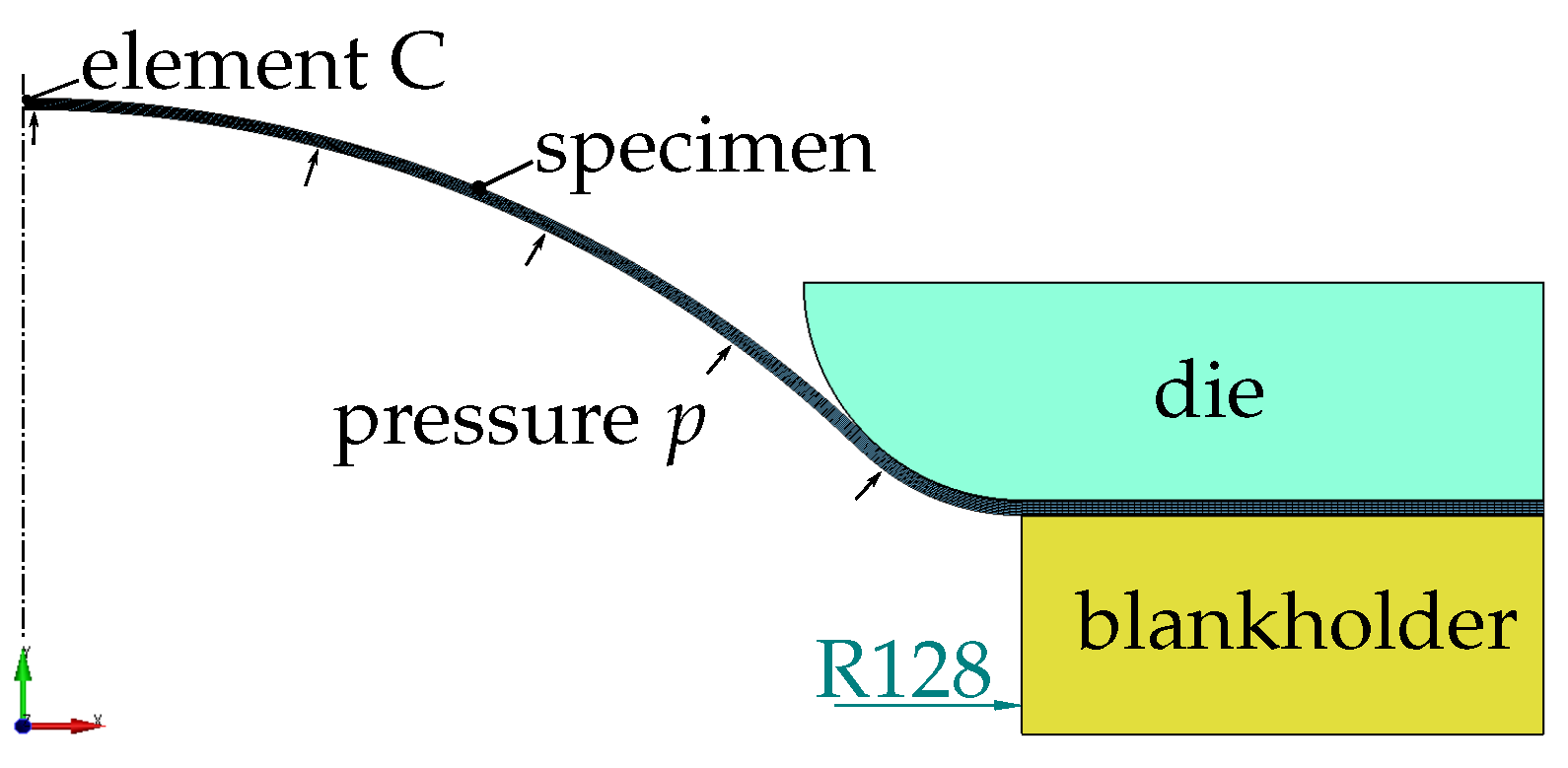
Another test method for determining the flow curve of sheet metal materials is the layer compression test (LCT), which is an adaptation of the classical compression test (DIN 50106) to sheet metal materials [35] and is characterised by a deviatoric biaxial stress condition. Instead of bulk material, the test specimens consist of a stack of sheet metal discs, as shown in Figure 3, since the initial raw material is a sheet metal [36]. The sheet metal discs are deformed between two parallel tool surfaces, which reduces the stack height [37]. It is characterised by a greater testing effort, such as the minimisation of friction between the tool and the specimen stack, as well as the uniform orientation of the sheet metal discs [38]. However, virtually homogeneous plastic strains of up to $0.7$ can be achieved, which provides a higher experimental validation of the flow behaviour [30]. Circular blanks with a diameter of 10 mm for HCT590X and 15 mm for EN AW-6014 T4 were employed. The blanks were stacked and aligned in such a way that their rolling direction coincided prior to the application of the DIC pattern. According to DIN 50106, the ratio between the stacking height ($h_0$) and the blank diameter ($d_0$) should be between $1.0$ and $2.0$. For EN AW-6014 T4, nine blanks with a thickness of 2.0 mm were stacked ($h_0/d_0=1.2$). The blanks, comprising HCT590X with a thickness of 1.5 mm, were stacked in seven ($h_0/d_0=1.05$). Based on DIN 50106, a strain rate of 0.001 s⁻¹ was chosen. The experimental setup is depicted in Figure 3a. The tests were conducted on a Zwick Z1484 tensile-compression testing machine, which has a maximum compression force of 200 kN [33]. The deformation of the stacks was quantified by two 3D DIC systems, as shown in Figure 3b, which were positioned at a 90° angle to each other [13]. This arrangement allowed for the measurement of material anisotropy, as it resulted in an elliptical deformation of the stack. For accurate testing, a proper cylindrical alignment of the discs and constant orientation of the rolling direction must be ensured.

The layer compression test enhances the calibration of the flow stress as it obtains uniform strains of up to $0.6$, well beyond the tensile tests. However, due to its strong uniform compression and lack of observable damage and failure, it cannot provide information on failure calibration.

2.2.4. Bulge Test

The bulge test, illustrated in Figure 4a, involves the clamping of a circular specimen between a die and a blankholder. Pressure is applied through a fluid and results in the deformation of the blank enclosed by the ring-shaped die. In contrast to the previous experiments, the loading in this instance was pressure-controlled. As the specimen is clamped, material reflowing is prevented, resulting in elongation. This is accompanied by simultaneous thinning, leading to a biaxial tensile stress. Once again, the deformation was measured by digital image correlation, as depicted in Figure 4b. The test was conducted up to the fracture of the sample, which occurred around the middle of the circular blank, as shown in Figure 4c. One advantage of the bulge test is that it allows for the investigation of the material behaviour at higher plastic strains up to $0.8$ [30]. Furthermore, the test setup can be assumed to be friction-free due to the hydraulic active medium. One particular challenge during testing is the control of the strain rate, as demonstrated in [39], in order to achieve a constant value and avoid significant effects on the biaxial stress–strain curve of materials [13]. The experiments conducted herein were initially meant for plasticity characterisation of the materials at hand; thus, they were conducted with a low DIC frame rate of 1 Hz. This was chosen because the test was performed in a strain-controlled manner using optical strain measurement. Higher measurement rates require significantly more computing power and cannot be realised with the systems used. However, for the highly ductile materials considered, the applicable pressure decreased before fracture initiation. As the loading was applied by increasing the pressure, the control system could produce sudden changes, accelerating fracture. This, combined with the low frame rate, causes the highest measured strain during testing to typically be merely a lower bound on the actual failure strain.

The bulge test also obtains higher but non-uniform plastic strains, which is important for the calibration of plasticity. As the stress state at the critical failure location remains rather constant, it provides a steady point in stress space for calibration of the failure surface.

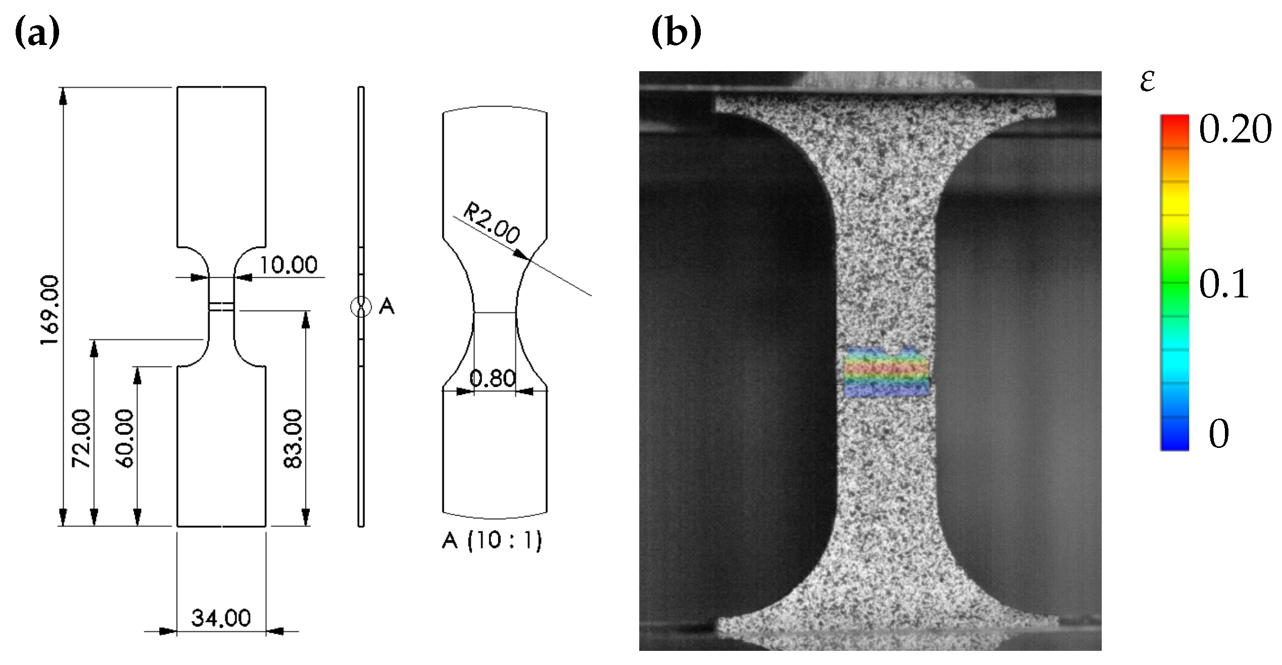
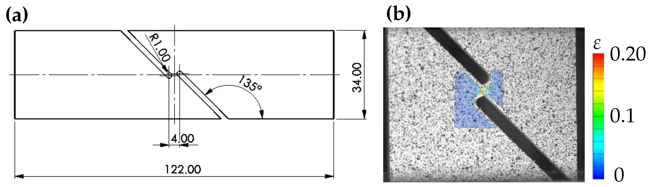
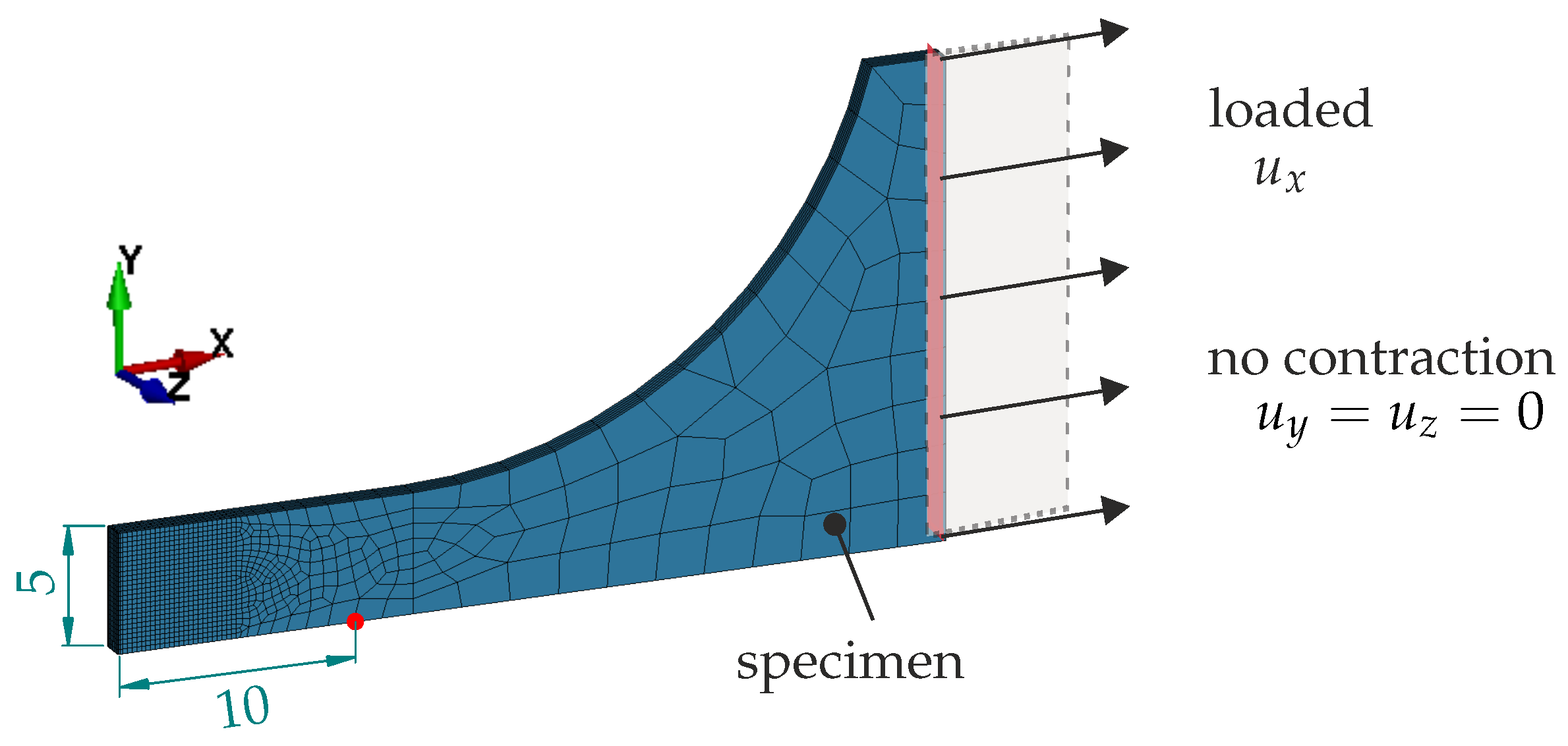
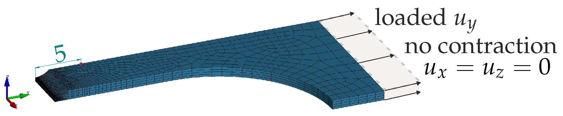
2.2.5. Mini-ASTM Shear Test

Shear tensile specimens were tested to introduce shear stress states for calibration. The geometric dimensions of the specimens, which are shown in Figure 5, are based on the ASTM shear specimen B831 [41]. The notches were aligned to form a −10° overlap to (at least initially) introduce a shear-compression loading. However, as such configurations with negative overlap angles often cause warping and buckling of the inner region, as for instance observed in [42,43], the bridge height was purposefully reduced to 4 mm (dimensions shown in Figure 5a, hence the prefix “mini”). Consequently, the sheared region was about 2 mm in height and thus in the order of the sheet thickness of 1.5, …, 2.0 mm, which was expected to avoid buckling. Both ends of the specimen were clamped in the Z100 tensile-compression testing machine without using the pivoted fixture from [41]. However, as the specimen geometry used was asymmetric, it was expected to rotate or shift perpendicular to the loading direction. Therefore, besides using DIC, as shown in Figure 5b, to measure the elongation of the specimen, it was also utilised to track the perpendicular jaw motion. This information is later applied and studied in the simulation model.

This shear tensile specimen rendered a shear loading crucial for assessing the assumed von Mises yield surface. The −10° notch alignment was expected to initially render a compressive shear loading, which eventually shifted towards positive triaxialities. This stress state change is characteristic of many metal forming applications and is important for failure calibration.

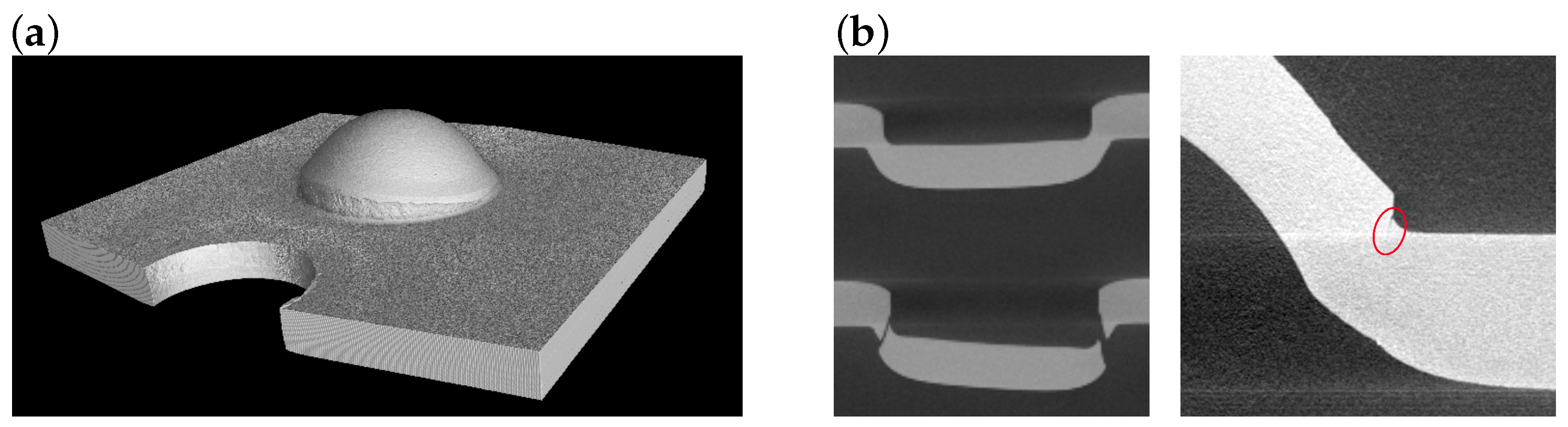
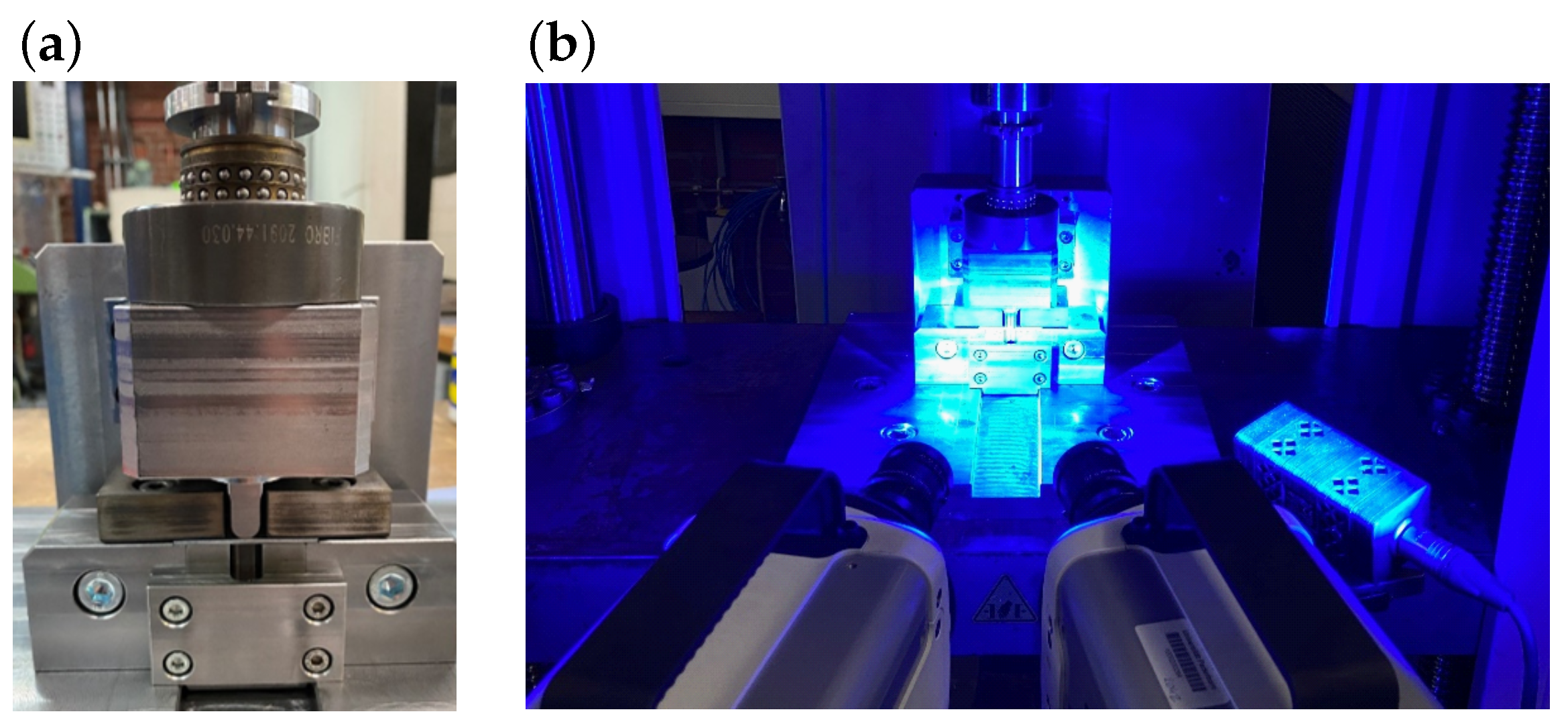
2.2.6. Classical Punch Test

In punch tests, the material is probed by pushing a punch into the clamped sheet. The experimental setup used for the classical punch test is depicted in Figure 6a. The boundary conditions and tool setup are similar to the targeted clinching process, so comparable loading and failure conditions were expected. Different variants are described, for instance, in [11] for the identification of failure parameters. By varying the geometric dimensions of the tools, such as the punch geometry in [44], different loading conditions and stress states are induced in the sheet material so different failure mechanisms can also be observed. Here, a flat punch (punch 3 used in Section 2.2.7, “PTf”) and a round punch (punch 4 used in Section 2.2.7, “PTr”) were used to capture low and high triaxialities. Both variants were applied to probe the aluminium alloy but not the dual-phase steel. The indentation depth of the punch was recorded by DIC, using the point markers shown in Figure 6b.

For such classical punch tests, however, the failure behaviour in the sheet plane behind the front surface cannot be detected with common optical methods. As a result, the exact determination of the crack initiation time and location is not always possible. Even though it is possible to deploy ex situ computed tomography [45,46] to immerse into the material and detect the crack, as realised in Figure 7, such an elaborate approach is costly.

Nevertheless, classical punch tests achieve important loading conditions by incorporating compression to approach the targeted application. Higher but non-uniform plastic strains are reached, which, together with the flexibility of the setup, can enhance the calibration of the failure surface.

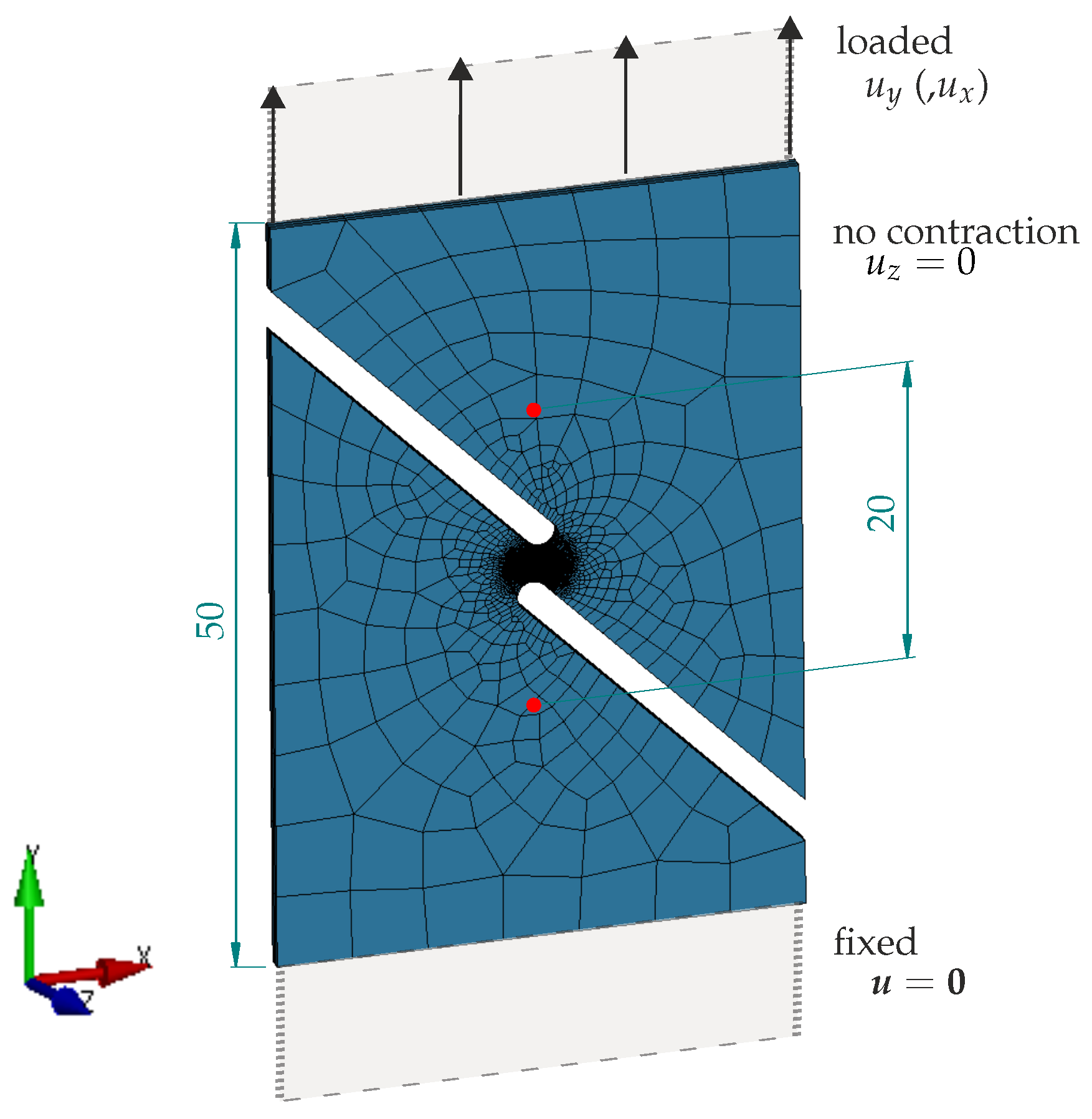
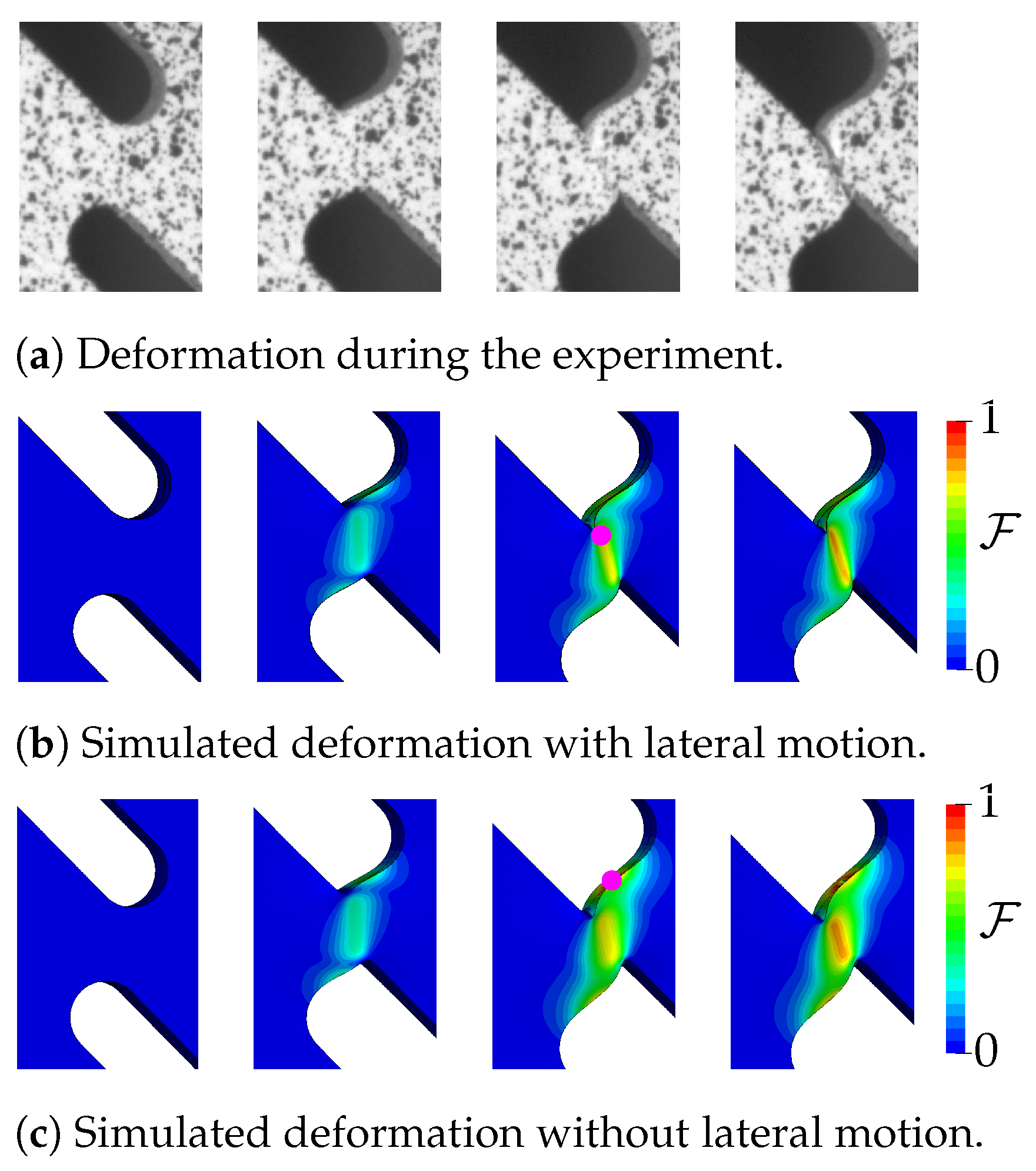
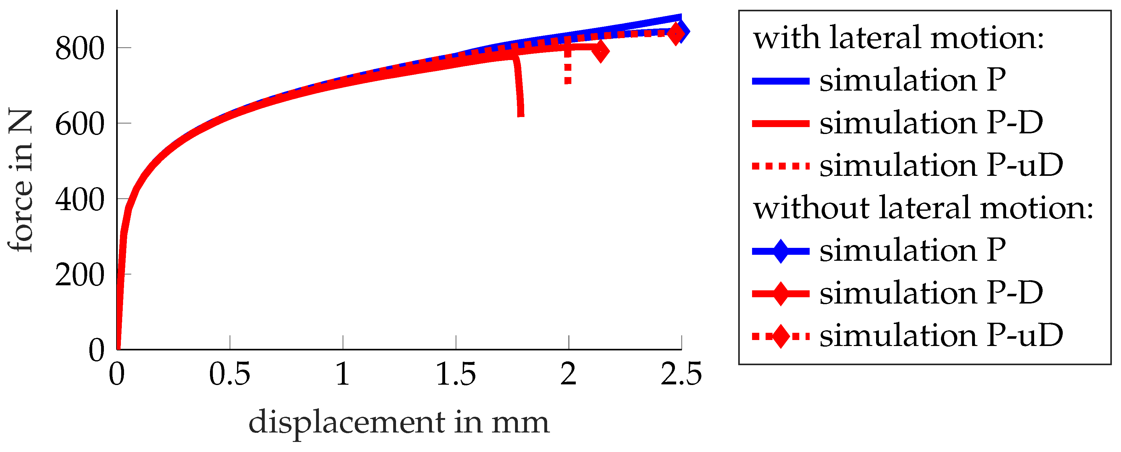
2.2.7. Modified Punch Test

To simplify the precise determination of the crack initiation time and location and maintain the versatility of the punch test, a modified punch test (MPT) was developed [12]. It involves penetrating the sheet directly at the edge with a punch and using DIC to record and evaluate the material failure in the sheet plane. For reproducing certain stress conditions, again, different geometries of the punch and die can be used [11,14].

The modified punch test, as well as the test setup with DIC using high-speed cameras, is shown in Figure 8. The test rig was again implemented in a Zwick Z100 universal testing machine. The axial force was applied by moving the system traverse. A GOM ARAMIS system was used to optically capture the deformation of the sheet edge and the crack initiation. In addition, the calibrated 3D DIC system was used to position the inserter in the spatial direction so that the punch tip was aligned exactly above the sheet edge. The design and detailed structure of the test can be found in [12].

Variants

The modified punch test can be employed to examine a range of punch types, as illustrated in Figure 9a. In the first instance, conventional cylindrical punches (“3D”), either blunt-nosed (“flat”) or hemispherical (“round”), can be utilised, as exemplified in Figure 9b. For this purpose, a conventional die is employed in a half-sectioned configuration. Additionally, rectangular bar-shaped punches (“2D”) can also be employed, which produce shear cutting-like deformation conditions, which are adjustable by the punch shape (“flat” or “round”), as shown in Figure 9c. In order to achieve this, a long pocket is created in the die, over which a strip of sheet metal is clamped that corresponds to the width of the punch.

Experimental Procedure

Due to the 3D DIC system, the displacements can be measured in all three directions, as shown in Figure 10. This enables the accurate alignment of the punch, sheet, and die. The sheet metal samples are clamped with serrated blankholders made of hardened steel. The serrated design prevents the sheet metal specimen from being drawn into the gap during the test. The blankholders are reproducibly tightened with screws and a defined torque for each test.

An important aspect that results from the kinematics of the test, which must be tracked carefully, is the z-displacement of the punch, where the motion is perpendicular to the view plane (towards the camera). As the punch presses on the sheet edge and the sample deforms plastically and bends downwards, the punch bends away from the sheet edge. This effect is particularly observable with the cylindrical round (“3D round”) punch (Figure 10b) and is more pronounced with the high-strength steel than with the aluminium material.

To sum up, the modified punch tests also provide crucial loading conditions, enhancing the identification of failure parameters. Thanks to the cut half-setup, the experimental setup is even more flexible and allows for direct visual access.

2.3. Numerical Setups

The simulation models used to reconstruct the previously outlined experiments are described in the following. LS-DYNA is used as finite-element solver, with all models solved using implicit time integration. Solid and axisymmetric continuum elements are applied for discretisation. The solid elements are trilinear 3D hexahedral 8-noded elements with reduced integration (ELFORM = 1) and suitable hourglass control (QH = 6, IHQ = 0.01), referred to hereafter as element parameter set A1. The 4-noded bilinear quadrilateral axisymmetric elements (ELFORM = 15) with reduced integration and default hourglass control are referred to hereafter as element parameter set A2.

To reduce the computational effort, especially for inverse parameter identification, symmetry constraints are regularly applied due to geometric symmetries. It must be emphasised, however, that this also enforces the localisation and failure patterns to be symmetric, which is generally not valid and typically cannot be enforced by the experimental setup. For simplicity and efficiency in inverse parameter identification, this effect is neglected for now.

2.3.1. Tensile Tests

The tensile test geometries are based on the A50 specimen from DIN 50125 [32], as shown in Figure 11, and on the SEP1230 setup from [31], as shown in Figure 12. In both cases, the meshes are locally refined to accurately capture strong necking and localisation towards the end of the loading. The minimum element size is 25 × 200 µm (in-plane x-, y-dimensions), with six elements used to discretise half of the sheet’s thickness. Element parameter set A1 is chosen. One-eighth of the 3D model is considered by utilising geometric symmetry and applying appropriate boundary conditions on the symmetry planes. On the right end in the x-direction, the load is imposed as a Dirichlet boundary condition by $u_x$ with constrained contraction, where $\mathit{u}$ describes the displacement vector with components $(u_x,u_y,u_z)$.

2.3.2. Plane-Strain Tensile Test

The plane-strain tensile test is modelled similarly to the tensile tests in Section 2.3.1 as a one-eighth model, as shown in Figure 13, with the same boundary conditions. Due to the notch in the thickness direction, strong necking is expected; thus, the mesh is refined in this region. The minimum element size is about 100 × 15 × 50 µm. Element parameter set A1 is chosen.

2.3.3. Layer Compression Test

The numerical setup for the layer compression test (LCT) is depicted in Figure 14. In contrast to the comprehensive simulation model (Figure 14, left) developed in [47] and applied in [48] for validation, here, a simplified setup is deployed. As anisotropy is neglected, the 3D quarter-model is reduced to an axisymmetric model. Moreover, based on investigations of the full model, the individual sheets with their own contact conditions can be replaced with a continuous cylinder. Due to geometric symmetry in the axial/y-direction, a half-model is sufficient. The resulting bottom face (y = 0) is constrained in the y-direction to model the symmetry plane. The upper tool is modelled as a rigid body and used to introduce frictional contact with a static friction coefficient of $0.01$, as in [47].

The height of the stack results from the sheet thickness and the number of layers, as described in Section 2.2.3. For the half-model, the heights are 9 mm for EN AW-6014 T4 and 5.25 mm for HCT590X. Due to the almost homogeneous deformation and the absence of fracture up to the applied compression of about 50%, the mesh is uncritical and chosen coarse. For this axisymmetric model, element parameter set A2 is used.

2.3.4. Bulge Test

Loading of the bulge test is controlled by prescribing the fluid pressure, as described in Section 2.2.4. However, as the considered metals are highly ductile, a snap-through occurs before final failure characterised by a decreasing applicable pressure. In the simulation, the load is identically applied by pressurising the sheet, as shown in Figure 15; thus, an arc-length method is required to apply the load and follow the load path up to fracture. This can be activated in LS-DYNA by an optional arc-length card, where a modified Crisfield method is selected.

As for the layer compression test, the setup is simplified to an axisymmetric model neglecting anisotropic effects and asymmetries during localisation and fracture. Element parameter set A2 is used. The ring-shaped die is depicted in Figure 15, which, together with the blankholder, clamps the sheet. It appears that the exact implementation of the clamping hardly affects the measured result. The load is applied by a linearly increasing pressure perpendicular to the bottom (y = 0) of the sheet and follows the deformation (follower-load). The accumulated plastic strain in element C at the top centre of the specimen, as marked in Figure 15, is measured and plotted against the applied pressure. Ten elements are used to discretise the sheet thickness, and the minimum element size is about 90 μm in x-direction for element C.

2.3.5. Mini-ASTM Shear Test

The bottom face (y = 0) of the specimen is fixed in all directions, as shown in Figure 16, while the top face is displaced upwards to induce shearing initially overlaid by compression in the inner region. Due to geometric symmetry in the sheet thickness direction, a half-model is considered. This hinders out-of-plane warping of the sheet in the simulation, which might occur in the experiment, as observed in [42,43]. However, as the height of the shear zone is purposefully reduced to obtain this mini-ASTM specimen, buckling and warping also appear to be effectively suppressed during the experiment. Element parameter set A1 is chosen.

The shear specimen is modelled with its full width and a free length between the clamping jaws. This is important as the asymmetry of the specimen causes its ends to slightly rotate or shift perpendicular to the loading direction. By modelling the specimen up to the clamping jaws, it becomes possible to apply the vertical and horizontal displacements close to the clamps, as measured by DIC. It is revealed that this lateral motion is essential for predicting the actual failure behaviour. Figure 17 depicts the deformation, and Figure 18 compares the global system response with ($u_x\ne 0$) and without ($u_x=0$, diamond marker) lateral motion for EN AW-6014 T4. The comparison includes responses for pure elastoplasticity (P), uncoupled plasticity–damage (P-uD), and coupled plasticity–damage (P-D). Without lateral motion, failure clearly occurs later and, more importantly, at a location besides the notch, as shown by the fracture initiation location (magenta dot) in Figure 17c. This location features a distinctly different stress state. The correct failure mode (Figure 17a) is only obtained in the simulation (Figure 17b) when lateral motion is taken into account. Thus, lateral motion is measured during the experiment and applied to the simulations in Section 2.4 for HCT590X and EN AW-6014 T4.

The lateral jaw motion was measured for the actual material response but is prescribed as a boundary condition for both the elastoplastic material model and the model with softening due to damage. For elastoplasticity without softening, the jaw motion is unrealistic as it is dominated by the stiffness decrease of the specimen during softening and failure. Nevertheless, the jaw motion is applied in both cases. A more realistic approach would model the actual machine stiffness to naturally obtain the lateral motion.

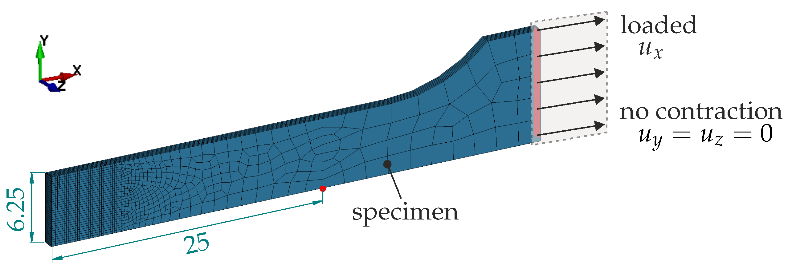
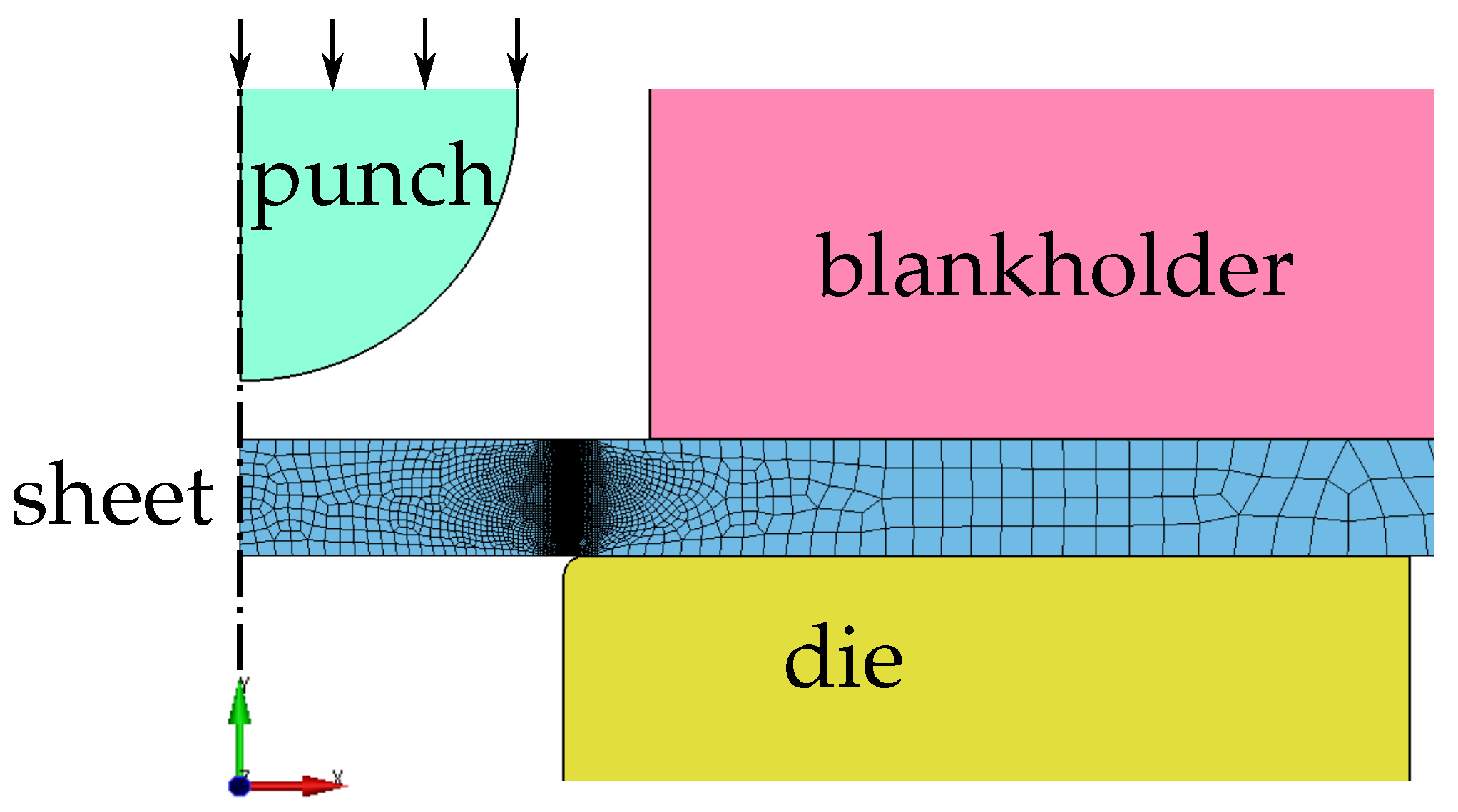
2.3.6. Classical Punch Test

Due to the closed symmetric setup of the classical punch test, axisymmetric modelling is possible. Element parameter set A2 is used. The tools (punch, die, and blankholder) are modelled as elastic bodies. Frictional contact is defined between the tools and the sheet specimen. Clamping of the sheet is realised by prescribing a force of 20 kN on the full blankholder to ensure minimal radial material inlet. The punch is displaced downwards in the negative y-direction by a prescribed displacement, and the required force is measured. Punch displacement against punch force plots are generated based on the simulation results. Two variants are considered: one with a flat punch (PTf, Figure 19) and one with a round punch (PTr, Figure 20). The minimum element size is about 20 μm.

2.3.7. Modified Punch Test

The modified punch test requires a 3D simulation model. However, due to symmetry in the x-direction, a half-model can be utilised, as shown in Figure 21. Again, it must be emphasised that this symmetry is a mere simplification, as during the experiment, the punch is observed to also slightly displace in the x-direction. The tools are modelled and loaded similarly to Section 2.3.6, and element parameter set A1 is chosen.

As described in Section 2.2.7, the sheet and tool alignment are measured by DIC and are applied in the simulation model. Also, the z-displacement of the punch is measured in the experiment and identically applied to the simulation model. Thanks to the open setup of the modified punch test, all these positions and deformations become visually accessible and can thus be measured and utilised in the simulation. This information is crucial for the correct reconstruction of the experiments, as the simulation results are sensitive to the tool alignment and displacement.

2.4. Material Parameter Identification Procedure

This section describes the general procedure for material parameter identification. First, Young’s modulus was measured using the LAwave measurement system developed at the Fraunhofer IWS [49]. It measures the elastic modulus based on laser-induced surface acoustic wave spectroscopy, enables non-destructive characterisation, and further facilitates direction-dependent measurements. The results are summarised in Section 3.1.1 and Section 3.2.1. The flow curve for plasticity governing the isotropic plastic hardening was identified based on layer compression tests and extrapolated suitably for clinching based on [33], as reiterated in Section 3.1.2 and Section 3.2.2. The parameters for the damage-induced softening of HCT590X were deduced from already available experimental results on a similar dual-phase steel DP600, as described in Section 3.1.3. Lastly, the parameters for the combined Cockcroft–Latham–Oh and Hosford–Coulomb failure model were determined by inverse parameter identification using LS-OPT. The simulation results were fitted to the experimental results for the global system response, such as the applied force versus elongation, by adjusting the failure parameters to obtain the best fit relating to all selected experiments. The LS-OPT setup is similar to [50]. This procedure was subsequently applied to the dual-phase steel HCT590X described in Section 3.1 and the aluminium alloy EN AW-6014 T4 described in Section 3.2.

3. Results and Discussion

In this section, the material parameters for the dual-phase steel HCT590X (Section 3.1) and the aluminium alloy EN AW-6014 T4 (Section 3.2) are identified and the results for all experiments are summarised and discussed. The raw data of the experimental and simulated global system responses is available as Supplementary Materials for all experiments and both metals. Finally, a teaser is provided on the application of the calibrated damage and failure model to the simulation of clinch joining in Section 3.3.

3.1. Dual-Phase Steel HCT590X

The dual-phase steel HCT590X belongs to the DP600 class, with a soft ferrite microstructure and hard martensite islands. It combines very good formability with high strength.

3.1.1. Elasticity: LAwave Measurements

The measured Young’s modulus is 205.8 GPa in the rolling direction. Poisson’s ratio is assumed to be $0.3$.

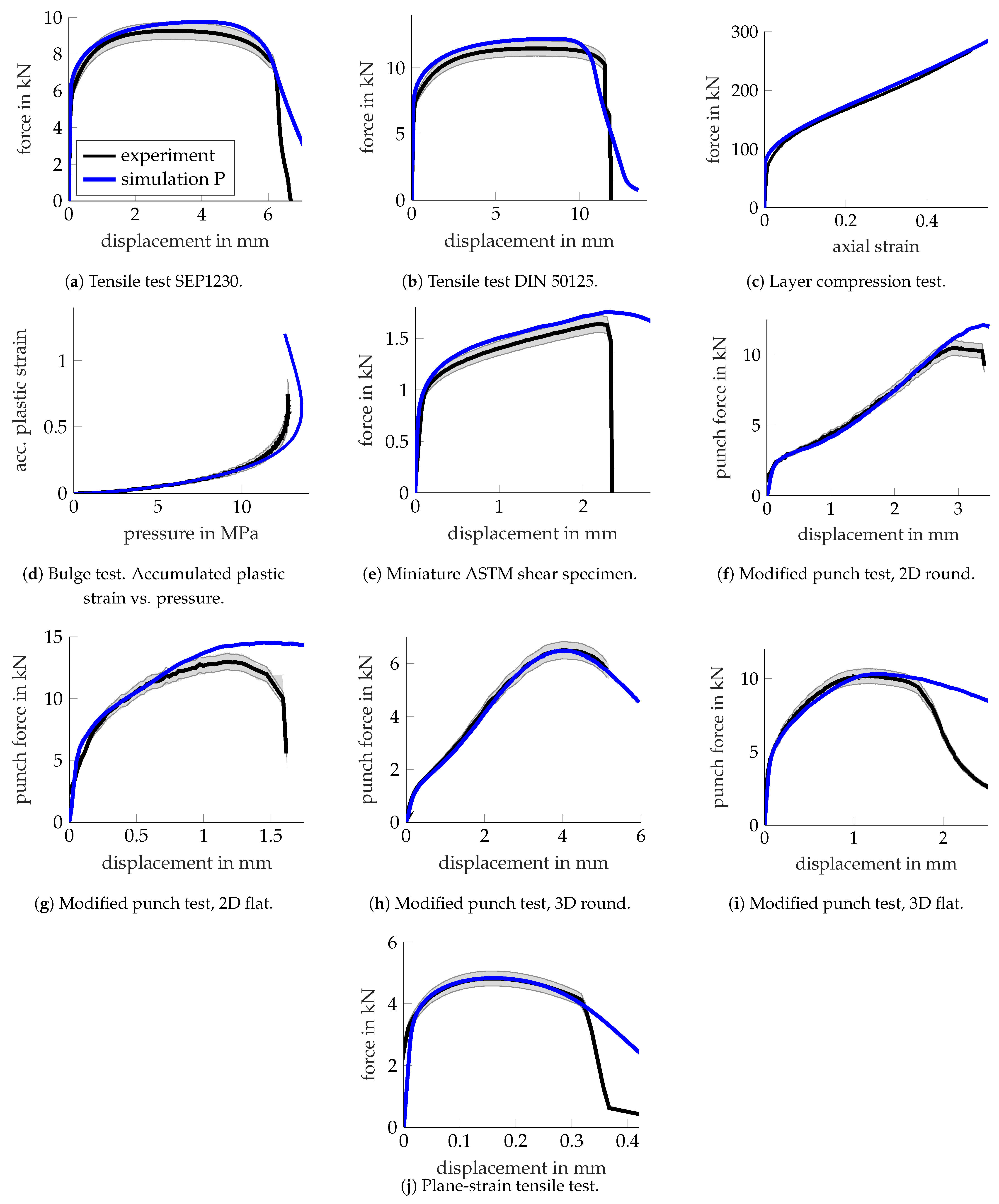
3.1.2. Plasticity: Verification and Limitations

The isotropic hardening behaviour is described by the flow stress equation stated in Equation (1) with six material parameters. These parameters are directly identified from a 1D curve fit to the extrapolated flow curve by [33] based on the layer compression test and are listed in

Table 3. HCT590X. Summary of material parameters for plasticity.

${\sigma }_{\mathrm{y}}$	K	$n_{\mathrm{p},K}$	$\mathrm{\Delta }{\sigma }_{y,\infty }$	$\omega$	$n_{\mathrm{p},\omega }$
$393.4$	$4.35$	$0.356$	$600.3$	$2.58$	$0.539$
MPa	MPa	–	MPa	–	–

.

Figure 22 depicts the global responses for 10 characterisation experiments (black) compared to the simulation results for pure elastoplasticity (blue).

Overall, the simulations for pure elastoplasticity obtained an acceptable match with the experimental results, thus verifying the material parameters for plasticity initially determined from layer compression tests, for a variety of stress states up to plastic strains of around 100%.

However, the comparison is also indicative of some shortcomings of the isotropic finite plasticity model used. First, comparing the tensile tests shown in Figure 22a,b to the layer compression test shown in Figure 22c, a plastic orthotropy might be conjectured. This is inherent to sheet metal, and even though the orthotropy is comparably small for the considered steel [48,51], it still causes around a 5% change in the flow stress depending on the sheet orientation. Second, the material appears to show a lower flow stress under shear loading, as shown in Figure 22e. This could be captured by a non-quadratic yield surface. However, the effect might also be entangled with plastic orthotropy. Lastly, comparing the results for the layer compression test shown in Figure 22c with those of the bulge test shown in Figure 22d, it is apparent that the bulge test appears to render smaller flow stress (lower sustained pressure) than the numerical prediction. This is surprising, as even for material models with anisotropic plasticity, both tests should typically render the same flow behaviour.

3.1.3. Damage to Failure Mapping

The mapping from the failure indicator to the damage variable was described in Section 2.1 and is determined by two parameters: the initial slope governed by the saturation parameter ${\eta }_{\mathrm{f}}$ and the critical failure indicator ${\mathcal{F}}^{\mathrm{crit}}$. Both parameters were deduced from a collection of experiments conducted by [19] on a congeneric dual-phase steel DP600, as re-iterated in Figure 23, including special micro-indentation tests. Therefore, a failure strain of $0.8$ was assumed based on Figure 23b. The measured damage values can be considered as mechanical damage, thereby describing the actual material degradation as incorporated by the damage variable into the simulation. However, these experimental results only provide a rough estimate of the amount of damage as, for instance, necking was present, causing a change in the stress state. Moreover, for simplicity, the underlying mapping was assumed to be identical for all stress states, so a reasonable compromise needs to be made, already taking into account the effect of damage on all the characterisation experiments in Section 3.1.4. By doing this, a critical failure indicator ${\mathcal{F}}^{\mathrm{crit}}=0.9$ and a saturation parameter ${\eta }_{\mathrm{f}}=0.05$ were deduced.

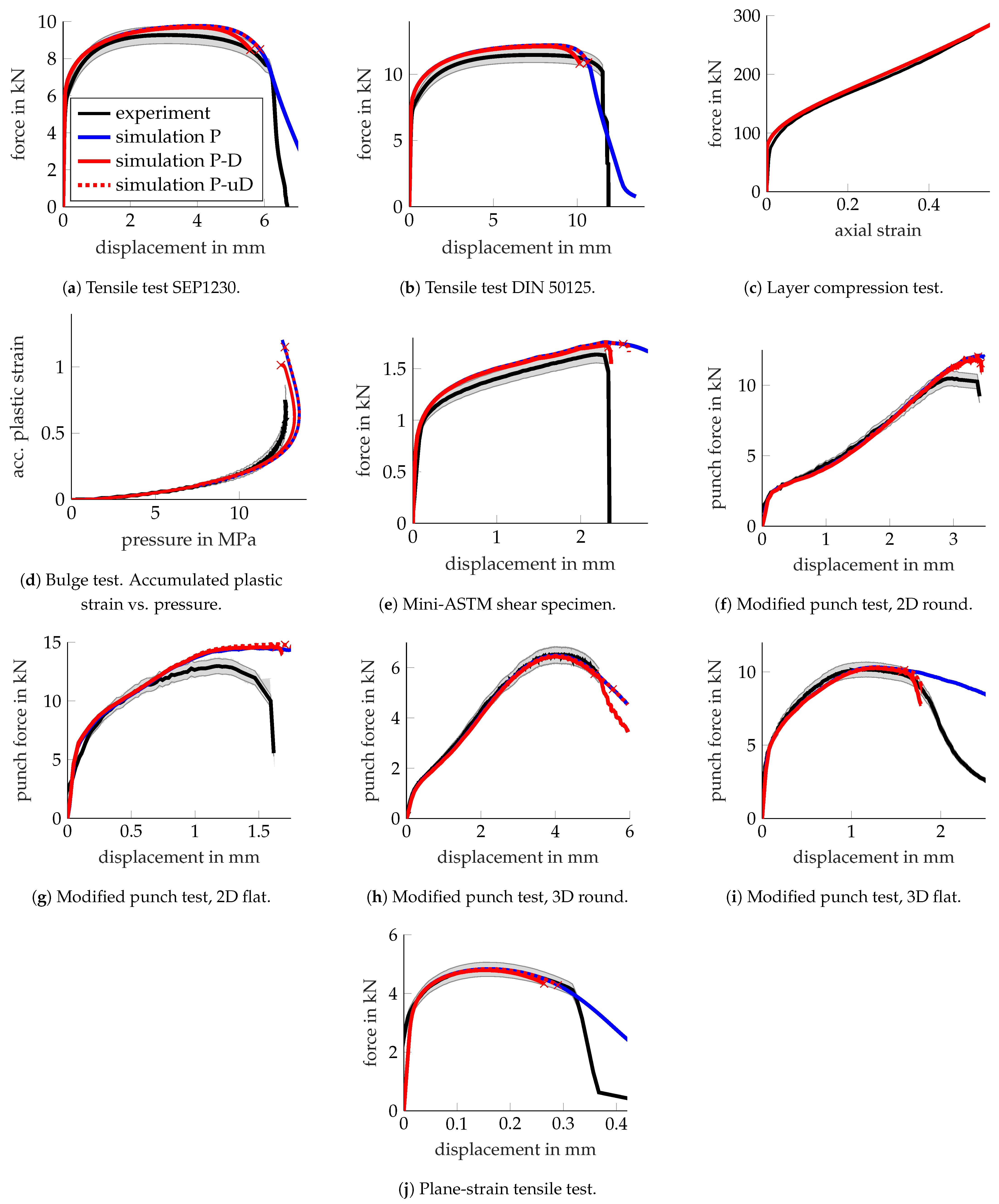
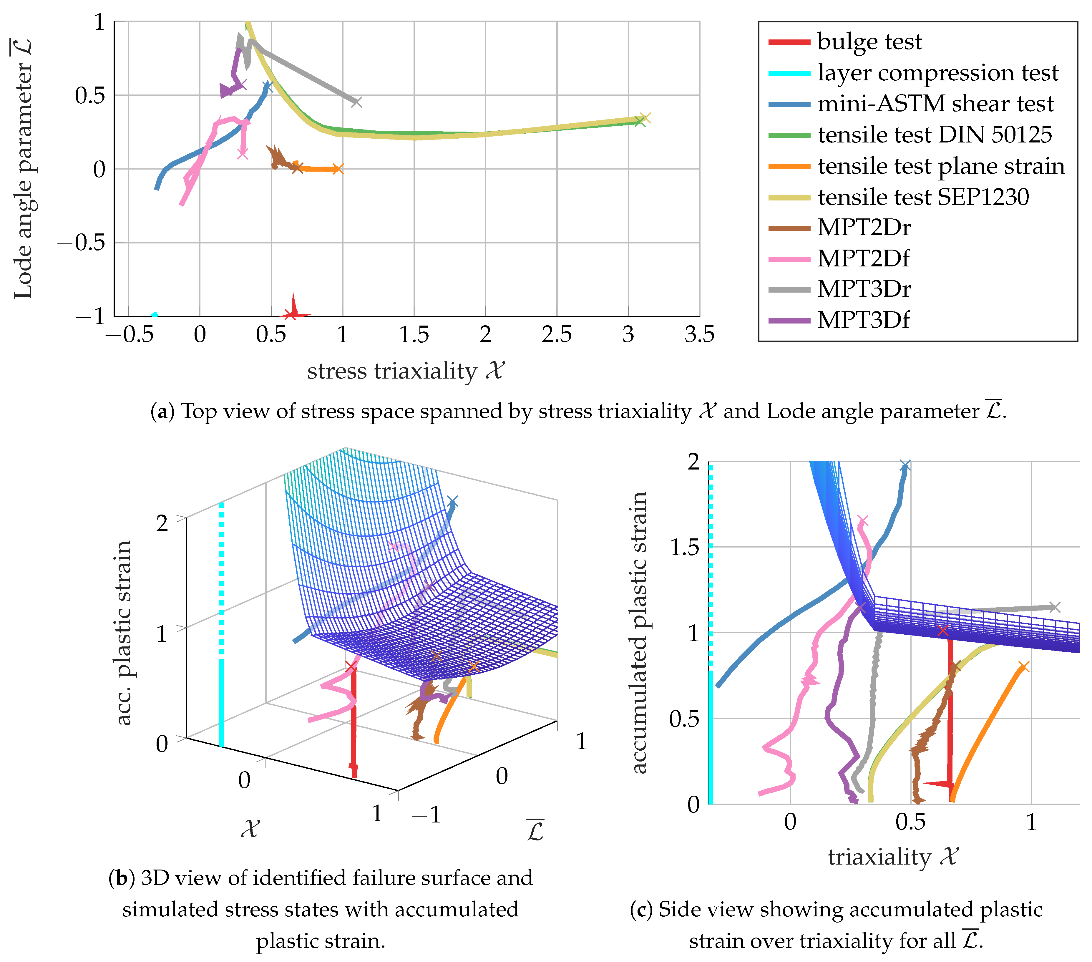
3.1.4. Failure: Inverse Identification

The failure parameters govern the upper bound for the damage evolution of the coupled plasticity–damage model and were obtained by inverse parameter identification. This is important and relevant for certain experiments, as the damage evolution affects the stress state, which, in turn, alters the damage accumulation up to failure. Figure 24 shows the global system responses for 10 experiments compared to the coupled plasticity–damage material model (P-D) with the optimised parameters in 

Table 4. HCT590X. Summary of failure parameters.

$a_{\mathrm{f}}$	$b_{\mathrm{f}}$	$c_{\mathrm{f}}$	$b_{\mathrm{CLO}}$	$n_{\mathrm{f}}$
$1.7$	$1.15$	$0.01$	$2.9$	$0.12$

.

An acceptable fit was obtained, where, for instance, the MPT3Dr, MPT3Df, and mini-ASTM experiments aligned well. It appears that the identification tried to find a balance between the MPT2Dr experiment, which was still overestimated, and the tensile tests, which were underestimated, as seen in the stress states in Figure 25c.

For comparison, the system responses for an uncoupled model (P-uD; red, dotted) were added, where damage caused no softening and the elements were abruptly deleted once the failure indicator reached the threshold of 1. For the MPT3Dr experiment, softening appeared to be important to predict the correct failure initiation. In the uncoupled model, failure was predicted notably later, resulting in lower identified failure strains. It appears that for all loadings where localisation was primarily driven by tension, the softening effect caused earlier failure. However, when the location of crack initiation was surrounded by compression, as in the MPT3Df experiment, softening played a minor role.

It appears that the final fracture did not occur for stress triaxiality $\mathcal{X}<0.2$ in the experiments. However, during clinching, this range is important, not because failure occurs there, but because no failure occurs for such low triaxiality, even at very high plastic strains of >2 (Section 3.3 and [52]). Therefore, it was necessary to manually increase the lower bound for the failure strain at pure shear defined by $b_{\mathrm{CLO}}$ during the inverse identification to ensure that failure strains were not underestimated in this stress range due to a lack of experimental data. Grain-based strain measurement [22] might be able to prove or disprove whether for $\mathcal{X}\approx 0$, such high strains can locally be reached without imminent failure.

The 10 experiments spanned a wide range of stress states, as summarised in Figure 25, where the stress triaxiality $\mathcal{X}$ and the Lode angle parameter $\overline{\mathcal{L}}$ are plotted for the crack initiation location (first representative element to fail). To remove the initial elastic behaviour and focus on the active evolution of the failure indicator, the plots start once the failure indicator is above $0.01$. The final fracture of the tracked elements is marked by “x”.

For the tensile tests, fracture initiation occurred at a triaxiality above 3. This can be attributed to the coupling of plasticity and damage, which caused the damage-induced softening to strongly increase the local triaxiality up to failure for highly ductile materials. This is in strong contrast to common assumptions of the triaxiality being constant at $1/3$ or only slowly increasing. Such high triaxialities at fracture could also explain the usual observation of pronounced voids on the fracture surface of tensile tests.

3.2. Aluminium Alloy EN AW-6014 T4

In this subsection, the aluminium alloy EN AW-6014 T4 is investigated with silicon and magnesium as major alloying elements. It is a precipitation-hardening alloy with excellent formability in the temper T4 condition. EN AW-6014 is widely used in industry, for instance, for automotive skin sheet applications. The general procedure for parameter identification described in Section 2.4 was identically applied in the previous subsection and is now rerun for the aluminium alloy.

3.2.1. Elasticity: LAwave Measurements

The measured Young’s modulus results in 70.4 GPa in the rolling direction. Poisson’s ratio is assumed to be 0.34.

3.2.2. Plasticity: Verification and Limitations

The isotropic hardening behaviour is described by the same flow stress equation stated in Equation (1) with six material parameters. These parameters were directly identified from a curve fit to the extrapolated flow curve by [33] and are listed in

Table 5. EN AW-6014 T4. Summary of material parameters for plasticity.

${\sigma }_{\mathrm{y}}$	K	$n_{\mathrm{p},K}$	$\mathrm{\Delta }{\sigma }_{y,\infty }$	$\omega$	$n_{\mathrm{p},\omega }$
$130.4$	$4.17$	$0.351$	$237.5$	$2.39$	$0.573$
MPa	MPa	–	MPa	–	–

.

Figure 26 depicts the global responses for 12 characterisation experiments (black), now including two variants of the classical punch test, compared to the simulation results for pure elastoplasticity (blue) and coupled plasticity–damage (red). Overall, an acceptable match was again obtained when comparing the experimental and numerical results, thus verifying the plasticity material parameters for a variety of stress states.

However, the comparison is once again indicative of some shortcomings of the isotropic finite plasticity model used for the aluminium alloy, similar to the findings in Section 3.1.2. The comparison of the results for EN AW-6014 T4 hints at the presence of plastic orthotropy. Anisotropy coefficients for this alloy were measured in [48] and analysed in [51]. The yield stress in the rolling direction (relevant for the tensile tests) was determined to be around 8% higher than in the sheet thickness direction (relevant for the layer compression test shown in Figure 26c). As plastic isotropy was assumed based on the layer compression test, the forces in the tensile tests (Figure 26a,b) were underestimated. The applied force in the mini-ASTM shear test shown in Figure 26e was again overestimated, likely due to the use of a quadratic yield surface, whereas aluminium is known to adhere more accurately, for instance, to a non-quadratic Hershey–Hosford yield surface [53]. The presence of a non-quadratic yield surface would also alter the simulation result for the plane-strain tensile test shown in Figure 26j and help reduce the current overprediction of the force. Comparing the experimental results and the simulation for the bulge test (Figure 26d) was again surprising, as the simulation underestimated the experimental result for the pressure. In contrast to the results for the dual-phase steel, it is now clear that the difference in the tension and compression responses cannot be directly used for damage quantification, as done in [54].

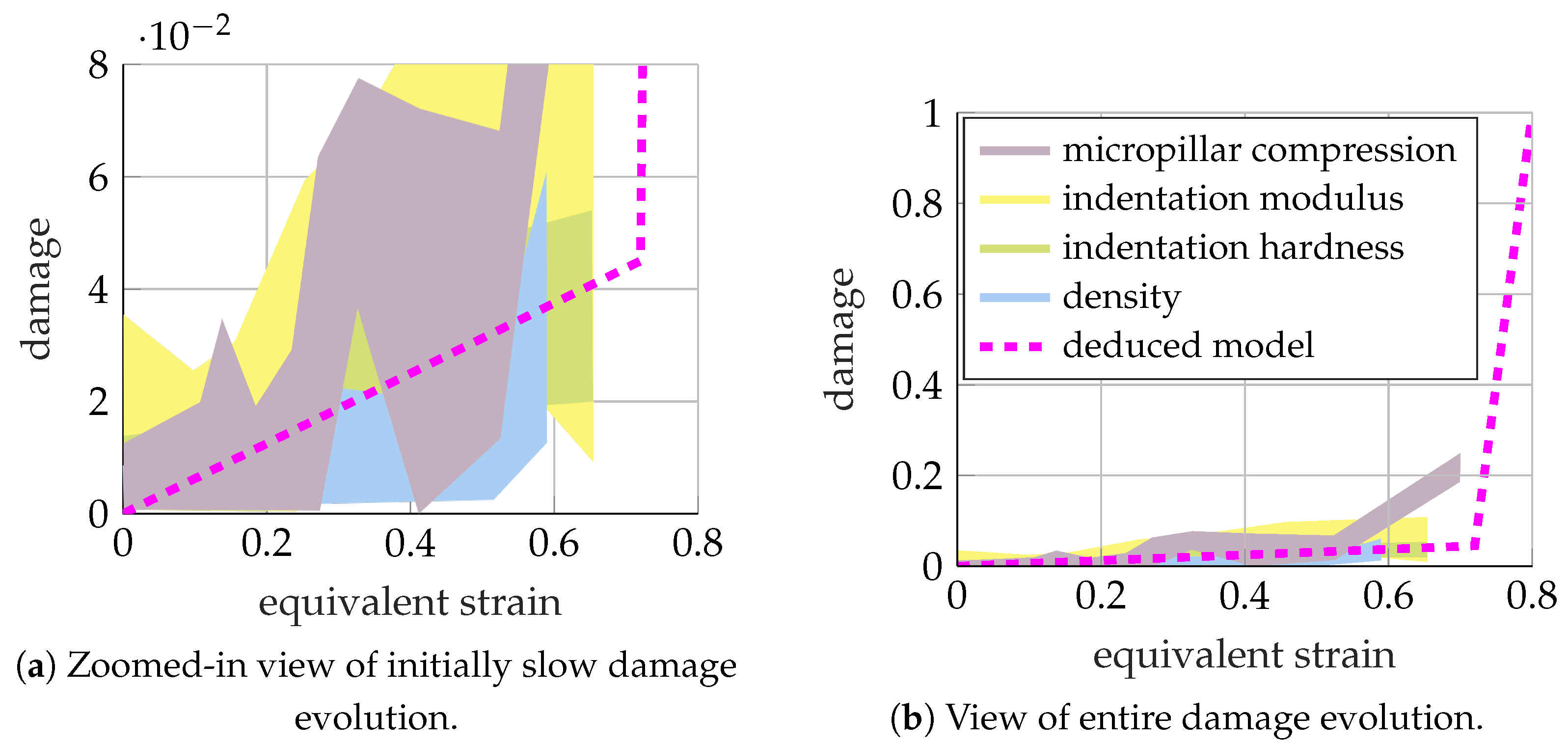
3.2.3. Damage to Failure Mapping: Deduction

Due to a lack of experimental results on actual mechanical damage measurements of a congeneric aluminium alloy, the damage parameters for the EN AW-6014 T4 were selected to be identical to those of the HCT590X deduced in Section 3.2.3.

3.2.4. Failure: Inverse Identification

The failure parameters were again fitted by inverse parameter identification based on the available results for all 12 experiments, rendering the fits in Figure 26. The inverse parameter identification was more challenging for this set of experiments. For instance, the results for the 3D flat modified punch test (MPT3Df, Figure 26i) were difficult to align with other experiments that caused similar stress states. It is difficult to conjecture the cause of this difference, even with the direct visual access provided by DIC. High-resolution microsections of stepwise loading tests might help increase the resolution of the critical location experimentally. The remaining differences between the experimental and numerical results depict no clear trend, with the displacement at failure sometimes being over- or underestimated. Moreover, the optimisation seemed to suffer from multiple local minima, as somewhat different combinations of failure parameters (“optimal” set summarised in

Table 6. EN AW-6014 T4. Summary of failure parameters.

$a_{\mathrm{f}}$	$b_{\mathrm{f}}$	$c_{\mathrm{f}}$	$b_{\mathrm{CLO}}$	$n_{\mathrm{f}}$
$1.5$	$0.8$	$0.01$	$1.4$	$0.155$

) rendered a shifted but comparably good fit to the experiments. Thus, it proved challenging to confine the material parameters.

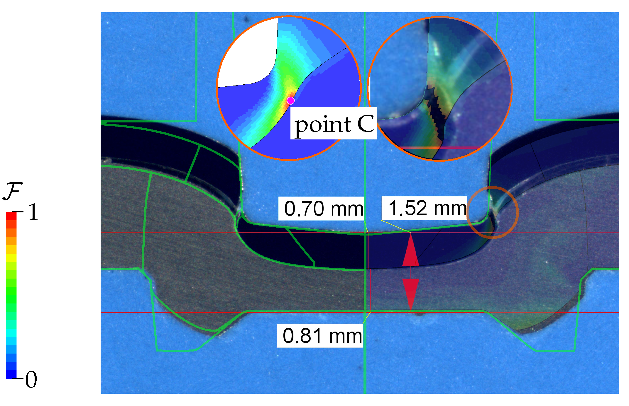
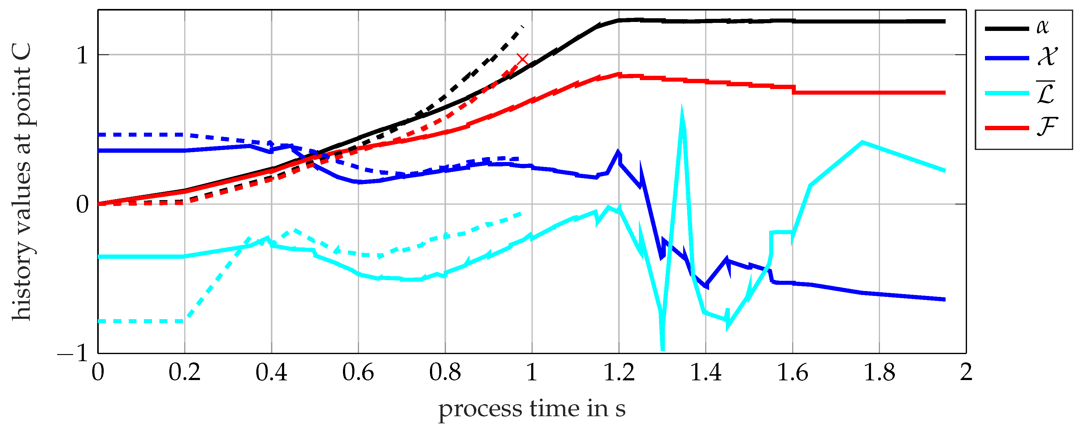
3.3. Towards Validation: A Teaser on Clinching

The calibrated material models are applied to the simulation of clinch joining in this section. One material combination is investigated to proceed with the validation of the model and the material parameters. Here, the focus is on the fracture of the dual-phase steel HCT590X, as the aluminium alloy typically does not fail during the clinch joining process, thus merely providing a lower bound for the failure strains.

An axisymmetric simulation was set up in LS-DYNA to model the joining process, as depicted exemplarily in Figure 27. The full cross-section is shown, but only the right half is modelled in the axisymmetric setup. Essential parameters for the clinch joining simulation include the sheet material behaviour, friction behaviour, tool geometries, punch indentation depth, sheet thickness, blankholder force, and several numerical aspects such as element size. The element size in the critical region surrounding the joint’s neck was chosen to be around 20 μm and was maintained through repeated remeshing. Constant Coulomb friction coefficients in the range ($0.05\dots 0.17$) were chosen. Further details on the simulation model are omitted for brevity and can be found in [52].

Combination K6 was studied, which joins a thin 0.8 mm HCT590X punch-sided sheet with a 2.0 mm thick EN AW-6014 T4 die-sided sheet. A special ABY4816501005 punch was selected, paired with a standard TOX BB8008 die as tool kit A (K6A). This combination rendered a valid joint, as displayed in Figure 28 and confirmed by the simulation with a maximum failure indicator of $0.88<1$, such that no fracture was predicted. Figure 28 compares the simulation results to a microsection of the joint, where good agreement with respect to the joint’s contour is observed. However, once a standard TOX A48100 conical punch was chosen as tool kit B (K6B), the punch-sided sheet fractured during forming, as indicated by the microsection in Figure 29. The coupled plasticity–damage material model calibrated herein was able to successfully reproduce this fracture occurring during the clinch joining process. Point C in Figure 29 marks this critical location, which is investigated in Figure 30 for both variants. There, the evolution of the accumulated plastic strain $\alpha$, the failure indicator $\mathcal{F}$, and the stress state is examined. The stress state fluctuates around $\mathcal{X}\approx 0.3$ and $\overline{\mathcal{L}}\approx -0.5$. The failure strain for a similar triaxiality was identified from the modified 3D round punch test, where the Lode angle parameter was about 1, which should render a higher failure strain due to the Lode valley. With an uncoupled failure model, the fracture strain would have been calibrated more than 10% lower from this experiment compared to [9], thus incorrectly predicting fracture. This indicates that the coupling of plasticity and damage helped capture the strong strain localisation towards fracture in the characterisation experiments and improved the identification of the failure strain. On the other hand, the influence of coupling plasticity and damage on the results of the clinching simulation appeared to be minor, such that the coupled and uncoupled models predicted very similar evolutions at the critical points. This might be a consequence of the strong geometric constraints and compression during clinching, which limited strain localisation, reduced the damage-softening effect, and thus yielded comparably high strains at failure for both models.

In [52], the applicability and validity of the material model and the parameters identified herein are further underscored by successfully studying around 20 different combinations for clinching both materials with a variety of tools and sheet thicknesses, as part of a versatile process chain [2].

4. Conclusions and Outlook

A stress-state-dependent ductile damage and failure model was successfully calibrated for two ductile metals. Up to 12 experiments were considered to span a variety of stress states. Attention was also devoted to compressive loading and non-proportional loading paths, which were directly embedded in the accumulation of the underlying failure indicator. The finite plasticity model used to describe material forming was fully coupled to a ductile damage model to phenomenologically describe the associated material degradation. This coupling can also notably affect the stress state up to fracture and improve the predictability of the model.

Besides classical characterisation experiments, such as tensile tests, more advanced setups, such as the modified punch test, were also incorporated into the calibration to bring it closer to the targeted application. It became clear that valid simulation models are a prerequisite for subsequent failure parameter identification. For instance, for the modified punch test, it is crucial to track the actual sheet and tool alignment, as well as motion, as these decisively affect fracture initiation and thus the identification. The same holds true for the desired application. Even for apparently simple tests, such as the shear specimen, it was revealed that the lateral motion of the two ends of the specimen needs to be tracked and identically applied in the simulation for correct failure prediction.

A teaser was provided for the targeted application of this model to the simulation of clinch joining, which is characterised by many of the above-considered features. A challenging material and sheet thickness combination was probed to confirm the applicability. A broader and more detailed investigation of a variety of clinching combinations is provided in [52].

The original model, developed in [9], was further regularised by a gradient enhancement of the damage variable. Such a regularisation introduces a length scale and is necessary for a coupled plasticity–damage model, as the damage-induced softening causes a pathological and unphysical mesh dependence of the finite-element results. In [9], it was shown that such a model is applicable, for instance, to the modified punch test, even when a realistic internal length scale is chosen, which is important for the correct prediction of damage and failure. However, this requires element sizes in the order of a few micrometres and causes numerical difficulties and high computational effort. Therefore, a gradient enhancement is not applied herein, and it is instead relied on suitable mesh designs. Future work could build on this point by developing suitable element formulations and increasing computational resources, or by investigating alternative localisation limiters.

Especially for highly ductile materials, where strong strain localisation precedes final fracture, the true local strain at fracture is challenging to determine [22,23]. Digital image correlation is inherently limited by the gauge length [21] and can decisively underestimate the strain at fracture. Electron backscatter diffraction and microsections could be suitable tools to study strain localisation close to fracture in greater detail at the grain-size level. Based on this, grain-based strain measurements can be performed to determine a lower bound for the strain at fracture [22] on a length scale defined by the material. Moreover, this might allow to distinguish possible damage-induced softening from a force decrease due to internal cracks and prove or disprove the predicted high failure strains at shear.

References

1. Tekkaya, A.; Bouchard, P.O.; Bruschi, S.; Tasan, C. Damage in metal forming. CIRP Ann. 2020, 69, 600–623. [Google Scholar] [CrossRef]
2. Meschut, G.; Merkein, M.; Brosius, A.; Bobbert, M. Mechanical joining in versatile process chains. Prod. Eng. 2022, 16, 187–191. [Google Scholar] [CrossRef]
3. Schramm, B.; Friedlein, J.; Gröger, B.; Bielak, C.; Bobbert, M.; Gude, M.; Meschut, G.; Wallmersperger, T.; Mergheim, J. A Review on the Modeling of the Clinching Process Chain-Part II: Joining Process. J. Adv. Join. Process. 2022, 6, 100134. [Google Scholar] [CrossRef]
4. Wciślik, W.; Lipiec, S. Void-Induced Ductile Fracture of Metals: Experimental Observations. Materials 2022, 15, 6473. [Google Scholar] [CrossRef] [PubMed]
5. Liang, J.; Zhang, M.; Peng, Y.; Wang, J. Advances in Understanding the Evolution Mechanism of Micropore Defects in Metal Materials under External Loads. Metals 2024, 14, 522. [Google Scholar] [CrossRef]
6. Bridgman, P.W. Studies in Large Plastic Flow and Fracture: With Special Emphasis on the Effects of Hydrostatic Pressure; Harvard University Press: Cambridge, MA, USA, 1964. [Google Scholar]
7. Bao, Y.; Wierzbicki, T. On fracture locus in the equivalent strain and stress triaxiality space. Int. J. Mech. Sci. 2004, 46, 81–98. [Google Scholar] [CrossRef]
8. Brünig, M.; Gerke, S.; Koirala, S. Biaxial experiments and numerical analysis on stress-state-dependent damage and failure behavior of the anisotropic aluminum alloy EN AW-2017A. Metals 2021, 11, 1214. [Google Scholar] [CrossRef]
9. Friedlein, J.; Mergheim, J.; Steinmann, P. Modelling of stress-state dependent ductile damage with gradient-enhancement exemplified for clinch joining. 2024, under review.
10. Bouchard, P.O.; Bourgeon, L.; Fayolle, S.; Mocellin, K. An enhanced Lemaitre model formulation for materials processing damage computation. Int. J. Mater. Form. 2011, 4, 299–315. [Google Scholar] [CrossRef]
11. Buyuk, M. Development of a Tabulated Thermo-Viscoplastic Material Model with Regularized Failure for Dynamic Ductile Failure Prediction of Structures under Impact Loading. Ph.D. Thesis, The George Washington University, Washington, DC, USA, 2013. [Google Scholar]
12. Böhnke, M.; Bielak, C.R.; Bobbert, M.; Meschut, G. Development of a Modified Punch Test for Investigating the Failure Behavior in Sheet Metal Materials. In Proceedings of the 12th International Conference and Workshop on Numerical Simulation of 3D Sheet Metal Forming Processes; Springer: Cham, Switzerland, 2022; pp. 575–584. [Google Scholar]
13. Kupfer, R.; Köhler, D.; Römisch, D.; Wituschek, S.; Ewenz, L.; Kalich, J.; Weiß, D.; Sadeghian, B.; Busch, M.; Krüger, J.; et al. Clinching of aluminum materials–methods for the continuous characterization of process, microstructure and properties. J. Adv. Join. Process. 2022, 5, 100108. [Google Scholar] [CrossRef]
14. Böhnke, M.; Bielak, C.R.; Friedlein, J.; Bobbert, M.; Mergheim, J.; Meschut, G.; Steinmann, P. A calibration method for failure modeling in clinching process simulations. Sheet Met. 2023, 25, 271. [Google Scholar]
15. Ghahremaninezhad, A.; Ravi-Chandar, K. Crack nucleation from a notch in a ductile material under shear dominant loading. Int. J. Fract. 2013, 184, 253–266. [Google Scholar] [CrossRef]
16. Cao, T.S. Numerical simulation of 3D ductile cracks formation using recent improved Lode-dependent plasticity and damage models combined with remeshing. Int. J. Solids Struct. 2014, 51, 2370–2381. [Google Scholar] [CrossRef]
17. Roth, C.C.; Mohr, D. Determining the strain to fracture for simple shear for a wide range of sheet metals. Int. J. Mech. Sci. 2018, 149, 224–240. [Google Scholar] [CrossRef]
18. Butcher, C.; Abedini, A. On phenomenological failure loci of metals under constant stress states of combined tension and shear: Issues of coaxiality and non-uniqueness. Metals 2019, 9, 1052. [Google Scholar] [CrossRef]
19. Tasan, C.; Hoefnagels, J.; Geers, M. Identification of the continuum damage parameter: An experimental challenge in modeling damage evolution. Acta Mater. 2012, 60, 3581–3589. [Google Scholar] [CrossRef]
20. Ghahremaninezhad, A.; Ravi-Chandar, K. Ductile failure behavior of polycrystalline Al 6061-T6. Int. J. Fract. 2012, 174, 177–202. [Google Scholar] [CrossRef]
21. Khameneh, F.; Abedini, A.; Butcher, C. Lengthscale effects in optical strain measurement for fracture characterization in simple shear. Int. J. Fract. 2021, 232, 153–180. [Google Scholar] [CrossRef]
22. Ghahremaninezhad, A.; Ravi-Chandar, K. Ductile failure behavior of polycrystalline Al 6061-T6 under shear dominant loading. Int. J. Fract. 2013, 180, 23–39. [Google Scholar] [CrossRef]
23. Scales, M.; Tardif, N.; Kyriakides, S. Ductile failure of aluminum alloy tubes under combined torsion and tension. Int. J. Solids Struct. 2016, 97, 116–128. [Google Scholar] [CrossRef]
24. Oh, S.; Chen, C.; Kobayashi, S. Ductile Fracture in Axisymmetric Extrusion and Drawing—Part 2: Workability in Extrusion and Drawing. ASME J. Eng. Ind. 1979, 101, 36–44. [Google Scholar] [CrossRef]
25. Mohr, D.; Marcadet, S.J. Micromechanically-motivated phenomenological Hosford–Coulomb model for predicting ductile fracture initiation at low stress triaxialities. Int. J. Solids Struct. 2015, 67, 40–55. [Google Scholar] [CrossRef]
26. HCT590X, Material Data Sheet, Salzgitter Flachstahl, Salzgitter, Germany. Available online: https://www.salzgitter-flachstahl.de/fileadmin/mediadb/szfg/informationsmaterial/produktinformationen/kaltgewalztes_feinblech/deu/hct590x.pdf (accessed on 1 June 2024).
27. EN AW-6014 T4, Material Data Sheet Novelis Advanz™ 6F-e170, Novelis Global Automotive. 2019. Available online: https://de.novelis.com/product/novelis-advanz-6f-e170/ (accessed on 1 June 2024).
28. ISO 6892-1:2019-11; Metallic Materials—Tensile Testing—Part 1: Method of Test at Room Temperature. ISO: Geneva, Switzerland, 2019.
29. Kopp, R.; Wiegels, H. Einführung in die Umformtechnik; Verlag Mainz Aachen: Aachen, Germany, 1999. [Google Scholar]
30. Bruschi, S.; Altan, T.; Banabic, D.; Bariani, P.F.; Brosius, A.; Cao, J.; Ghiotti, A.; Khraisheh, M.; Merklein, M.; Tekkaya, A.E. Testing and modelling of material behaviour and formability in sheet metal forming. CIRP Ann. 2014, 63, 727–749. [Google Scholar] [CrossRef]
31. SEP 1230:2007-02; The Determination of the Mechanical Properties of Sheet Metal at High Strain Rates in High-Speed Tensile Tests. Verlag Stahleisen GmbH: Düsseldorf, Germany, 2007.
32. DIN 50125:2022-08; Testing of Metallic Materials—Tensile Test Pieces. Deutsches Institut für Normung e.V. (DIN): Berlin, Germany, 2019.
33. Böhnke, M.; Kappe, F.; Bobbert, M.; Meschut, G. Influence of various procedures for the determination of flow curves on the predictive accuracy of numerical simulations for mechanical joining processes. Mater. Test. 2021, 63, 493–500. [Google Scholar] [CrossRef]
34. Basaran, M. Stress state dependent damage modeling with a focus on the lode angle influence. Ph.D. Thesis, Lehrstuhl und Institut für Allgemeine Mechanik, Shaker Verlag, Aachen, Germany, 2011. [Google Scholar]
35. Merklein, M.; Kuppert, A. A method for the layer compression test considering the anisotropic material behavior. Int. J. Mater. Form. 2009, 2, 483–486. [Google Scholar] [CrossRef]
36. Graf, M.; Henseler, T.; Ullmann, M.; Kawalla, R.; Prahl, U.; Awiszus, B. Study on determination of flow behaviour of 6060-aluminium and AZ31-magnesium thin sheet by means of stacked compression test. In Proceedings of the IOP Conference Series: Materials Science and Engineering, Chemnitz, Germany, 6–7 March 2019; IOP Publishing: Bristol, UK, 2019; Volume 480, p. 012023. [Google Scholar]
37. Pawelski, O. Über das Stauchen von Hohlzylindern und seine Eignung zur Bestimmung der Formänderungsfestigkeit dünner Bleche. Arch. Für Eisenhüttenwesen 1967, 38, 437–442. [Google Scholar] [CrossRef]
38. Doege, E.; Meyer-Nolkemper, H.; Saeed, I. Fließkurvenatlas Metallischer Werkstoffe: Mit Fließkurven für 73 Werkstoffe und einer grundlegenden Einführung; Hanser: München, Germany, 1986. [Google Scholar]
39. Suttner, S.; Merklein, M. Experimental and numerical investigation of a strain rate controlled hydraulic bulge test of sheet metal. J. Mater. Process. Technol. 2016, 235, 121–133. [Google Scholar] [CrossRef]
40. Slota, J.; Spišák, E. Determination of flow stress by the hydraulic bulge test. Metalurgija 2008, 47, 13–17. [Google Scholar]
41. ASTM B831-19; Standard Test Method for Shear Testing of Thin Aluminum Alloy Products. ASTM: West Conshohocken, PA, USA, 2005.
42. Trondl, A.; Klitschke, S.; Boehme, W.; Sun, D.Z. Verformungs- und Versagensverhalten von Stählen für den Automobilbau unter crashartiger mehrachsiger Belastung. FAT-Schriftenreihe. 2016. Available online: https://www.vda.de/de/aktuelles/publikationen/publication/fat-schriftenreihe-283 (accessed on 19 July 2024).
43. Otroshi, M.; Rossel, M.; Meschut, G. Stress state dependent damage modeling of self-pierce riveting process simulation using GISSMO damage model. J. Adv. Join. Process. 2020, 1, 100015. [Google Scholar] [CrossRef]
44. Lee, Y.W. Fracture Prediction in Metal Sheets. Ph.D. Thesis, Massachusetts Institute of Technology, Cambridge, MA, USA, 2005. [Google Scholar]
45. Busch, M.; Hausotte, T. Application of an edge detection algorithm for surface determination in industrial X-ray computed tomography. Prod. Eng. 2022, 16, 411–422. [Google Scholar] [CrossRef]
46. Busch, M.; Butzhammer, L.; Hausotte, T. Herausforderungen bei computertomografischen Untersuchungen von Fügeverbindungen. Tech. Mess. 2022, 89, 83–88. [Google Scholar] [CrossRef]
47. Graser, M.; Lenzen, M.; Merklein, M. On the inverse identification of Lankford coefficients using geometrical changes under quasi-biaxial loading. Int. J. Mater. Form. 2019, 12, 1053–1061. [Google Scholar] [CrossRef]
48. Friedlein, J.; Wituschek, S.; Lechner, M.; Mergheim, J.; Steinmann, P. Inverse parameter identification of an anisotropic plasticity model for sheet metal. In Proceedings of the IOP Conference Series: Materials Science and Engineering, Stuttgart, Germany, 21 June–2 July 2021; IOP Publishing: Bristol, UK, 2021; Volume 1157, p. 012004. [Google Scholar]
49. Schneider, D. LAwave®—A Nondestructive Device for Testing Thin Films, Coatings and Material Surfaces by Laser Induced Surface Acoustic Waves. 2013. Available online: https://www.researchgate.net/publication/268034125_LAwaveR_-_A_Nondestructive_Device_for_Testing_Thin_Films_Coatings_and_Material_Surfaces_by_Laser_Induced_Surface_Acoustic_Waves?channel=doi&linkId=545f742f0cf2c1a63bfdb595&showFulltext=true (accessed on 19 July 2024).
50. Nahrmann, M.; Matzenmiller, A. Modelling of nonlocal damage and failure in ductile steel sheets under multiaxial loading. Int. J. Solids Struct. 2021, 232, 111166. [Google Scholar] [CrossRef]
51. Friedlein, J.; Bielak, C.; Böhnke, M.; Bobbert, M.; Meschut, G.; Mergheim, J.; Steinmann, P. Influence of plastic orthotropy on clinching of sheet metal. Sheet Met. 2023, 25, 133–140. [Google Scholar]
52. Friedlein, J.; Kalich, J.; Lüder, S.; Schmale, H.C.; Böhnke, M.; Schlichter, M.; Bobbert, M.; Meschut, G.; Steinmann, P.; Mergheim, J. Application of stress-state dependent ductile damage and failure model to clinch joining for a wide range of tool and material combinations. 2024, to be submitted.
53. Banabic, D. Sheet Metal Forming Processes: Constitutive Modelling and Numerical Simulation; Springer Science & Business Media: Berlin/Heidelberg, Germany, 2010. [Google Scholar]
54. Schowtjak, A.; Wang, S.; Hering, O.; Clausmeyer, T.; Lohmar, J.; Schulte, R.; Ostwald, R.; Hirt, G.; Tekkaya, A.E. Prediction and analysis of damage evolution during caliber rolling and subsequent cold forward extrusion. Prod. Eng. 2020, 14, 33–41. [Google Scholar] [CrossRef]
Figure 1. (a) Geometric dimensions of the tensile specimen according to DIN 50125 [32]. (b) Geometric dimensions according to SEP1230 [31]. (c) Experimental setup for tensile tests in Zwick Z100 tensile-compression testing machine. (d) Evaluation with digital image correlation (DIC) using optical strain measurement. (Reprinted with permission from [33]).
Jmmp 08 00157 g001
Figure 2. (a) Geometric dimensions of the plane-strain tensile specimen according to [34] for EN AW-6014 T4. For the HCT590X specimen, a minimum thickness at the centre of the groove of 0.6 mm instead of 0.8 mm is selected. (b) Strain evaluation using DIC.
Jmmp 08 00157 g002
Figure 3. (a) Experimental setup for layer compression tests (LCT) in the Zwick Z1484 tensile-compression testing machine with two DIC systems. (b) Evaluation with DIC using optical strain measurement. (Reprinted with permission from [33]).
Jmmp 08 00157 g003
Figure 4. (a) Functional principle of the hydraulic bulge test [13]. (b) Evaluation with DIC using optical strain measurement. (c) Specimen after failure [40].
Jmmp 08 00157 g004
Figure 5. (a) Geometric dimensions of the mini-ASTM shear tensile specimen adapted from [41]. (b) Strain evaluation using DIC.
Jmmp 08 00157 g005
Figure 6. (a) Experimental setup of the classical punch test. (b) Evaluation of the local punch displacement using DIC.
Jmmp 08 00157 g006
Figure 7. Ex situ computed tomography of punch test specimens. (a) Fractured specimen probed with a round punch (punch 4 used in Section 2.2.7, “PTr”). (b) Specimen probed with a flat punch (punch 3 used in Section 2.2.7, “PTf”) with crack location highlighted by red circle.
Jmmp 08 00157 g007
Figure 8. Experimental setup of the modified punch test (MPT). (a) Variant 2D round (MPT2Dr) [12]. (b) Recording with high-speed cameras.
Jmmp 08 00157 g008
Figure 9. (a) Different tools for the modified punch test to achieve various stress states in the sheet material. (1) “2D flat” punch. (2) “2D round” punch. (3) “3D flat” punch. (4) “3D round” punch. (5) “2D” die. (6) “3D” die. (b) Setup for 3D round modified punch test with punch 4 and die 6 [12]. (c) 2D round setup with punch 2 and die 5 [12].
Jmmp 08 00157 g009
Figure 10. Modified punch test, 3D round. (a) Alignment of punch, sheet, and die using 3D DIC. (b) Bending and shift of the cylindrical punch shown as punch displacement u z in the z-direction (towards the camera) during the test.
Jmmp 08 00157 g010
Figure 11. Tensile test DIN 50125—numerical setup. Symmetry boundary conditions are applied on the left, bottom, and rear faces. The red point marks the evaluation point for the elongation measurement, as in the experiment.
Jmmp 08 00157 g011
Figure 12. Tensile test SEP1230—numerical setup. Symmetry boundary conditions are applied on the left, bottom, and rear faces. The red point marks the evaluation point for the elongation measurement, as in the experiment.
Jmmp 08 00157 g012
Figure 13. Plane-strain tensile test—numerical setup. One-eighth model.
Jmmp 08 00157 g013
Figure 14. Layer compression test (LCT)—numerical setup. Simplification of the 3D quarter-model to a 2D axisymmetric half-model.
Jmmp 08 00157 g014
Figure 15. Bulge test—numerical setup. The specimen with an overall diameter of 390 mm is clamped by the die and blankholder. An intermediate deformed specimen is depicted with the applied pressure following the bulging.
Jmmp 08 00157 g015
Figure 16. Mini-ASTM shear test—numerical setup. The specimen is clamped at the bottom and elongated in the y-direction. To reproduce the experimentally measured shift of the clamping jaws, the top is additionally displaced in the x-direction. Only half of the sheet thickness is modelled by applying appropriate symmetry constraints on the rear face.
Jmmp 08 00157 g016
Figure 17. Mini-ASTM shear test—deformation. The deformation in the inner region is investigated. (a) Experimental deformation at four stages during the test. The simulation with lateral motion in (b) obtains a similar deformation and correct crack initiation location (magenta dot, failure indicator F = 1 ). When lateral motion is not taken into account in the simulation (c), neither deformation nor failure is predicted correctly. The full model is shown.
Jmmp 08 00157 g017
Figure 18. Mini-ASTM shear test—force–displacement responses for pure elastoplasticity (P), coupled plasticity–damage (P-D), and uncoupled plasticity–damage (P-uD). The coupled plasticity–damage (red, solid) model predicts earlier fracture due to the underlying damage-induced softening. Taking into account the relative lateral motion of the two ends of the specimen further accelerates fracture initiation and is crucial for predicting the actual failure location, as shown in Figure 17.
Jmmp 08 00157 g018
Figure 19. Classical punch test with a flat punch (PTf)—numerical setup. Only a cutout of the entire setup is shown where the tools actually extend further to the top, bottom, and right.
Jmmp 08 00157 g019
Figure 20. Classical punch test with a round punch (PTr)—numerical setup. Only a cutout of the entire setup is shown.
Jmmp 08 00157 g020
Figure 21. Modified punch test—numerical setup. A half-model is shown with symmetry with respect to the yz-plane. The sheet specimen is clamped between the die and the blankholder. The punch is displaced downwards in the negative y-direction. Here, the 3D round modified punch test (MPT3Dr) is depicted. The other three variants are obtained by exchanging the punch and/or die.
Jmmp 08 00157 g021
Figure 22. HCT590X—force-displacement responses. Experiments (black) vs. simulations for pure elastoplasticity (P; blue).
Jmmp 08 00157 g022
Figure 23. Damage evolution in dual-phase steel DP600 measured by [19] using four theoretically equivalent methodologies. The damage to failure mapping is deduced from these results to roughly capture the initial softening up to the critical failure indicator and the subsequent fast degradation up to material fracture.
Jmmp 08 00157 g023
Figure 24. HCT590X—force-displacement responses. Experiments (black) vs. simulations for pure elastoplasticity (P; blue), coupled plasticity-damage (P-D; red, solid), and uncoupled plasticity-damage (P-uD; red, dotted).
Jmmp 08 00157 g024
Figure 25. HCT590X—summary of simulated stress states for all 10 experiments, including modified punch tests (MPT). Plotted for failure indicator F > 0.01 . Results of the layer compression test are added for comparison even though F = 0 .
Jmmp 08 00157 g025
Figure 26. EN AW-6014 T4. Force–displacement responses—experiments (black) vs. simulations for pure elastoplasticity (P; blue) and coupled plasticity–damage (P-D; red). The simulated crack initiation is indicated by “x”.
Jmmp 08 00157 g026
Figure 27. Clinch joining—numerical setup for combination K6A. Axisymmetric model.
Jmmp 08 00157 g027
Figure 28. Clinch joining of K6A. The simulated final joint contour aligns well with the experimental result shown in the background. The maximum failure indicator is predicted as 0.88 < 1 , which confirms that no fracture occurs.
Jmmp 08 00157 g028
Figure 29. Clinch joining of K6B. The punch-sided sheet fractures in the simulation at a similar location and bottom thickness as in the experiment. The zoomed-in areas show the deformation when the crack initiates at point C and the final fracture.
Jmmp 08 00157 g029
Figure 30. Clinch joining of K6A (solid) and K6B (dashed)—comparison of element values in the critical points (C) of both joints. With tool kit K6B, fracture occurs at a process time of about 1 s. With the special punch of K6A, the stress triaxiality X evolves similarly but the Lode angle parameter L ¯ is lower and the accumulated plastic strain α increases more slowly The accumulated plastic strain for K6A stagnates starting at around 1.2 s as the material remains elastic. The values for α and the failure indicator F decrease unphysically from there on due to mapping errors during repeated remeshing.
Jmmp 08 00157 g030