
Mean Value-Amplitude Method for the Determination of Anisotropic Mechanical Properties of Short Fiber Reinforced Thermoplastics


Abstract
:1. Introduction
2. Material and Experiments
3. Resolving Layerwise Properties
4. Results
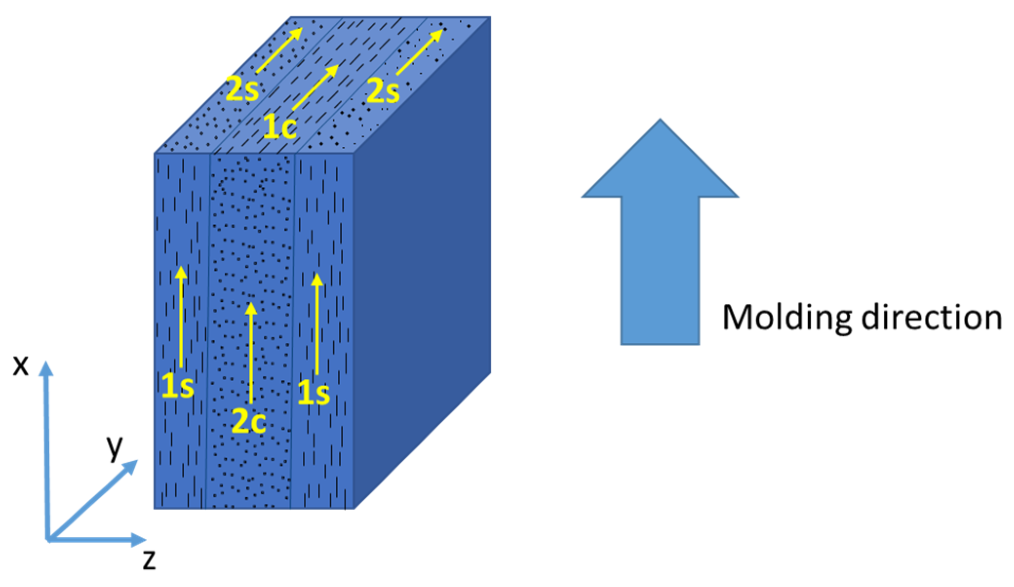
4.1. µCT-Analysis
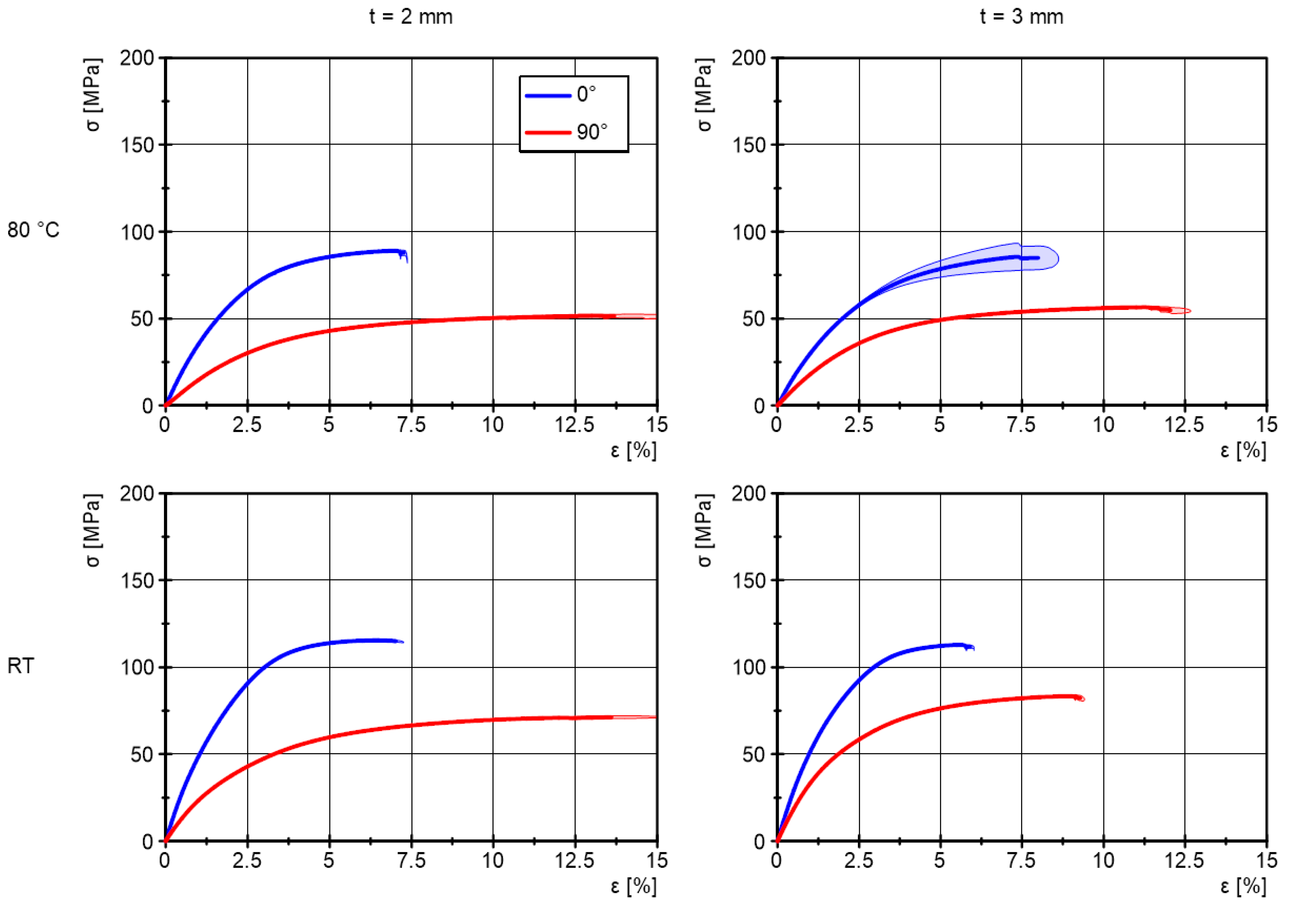
4.2. Tensile Tests
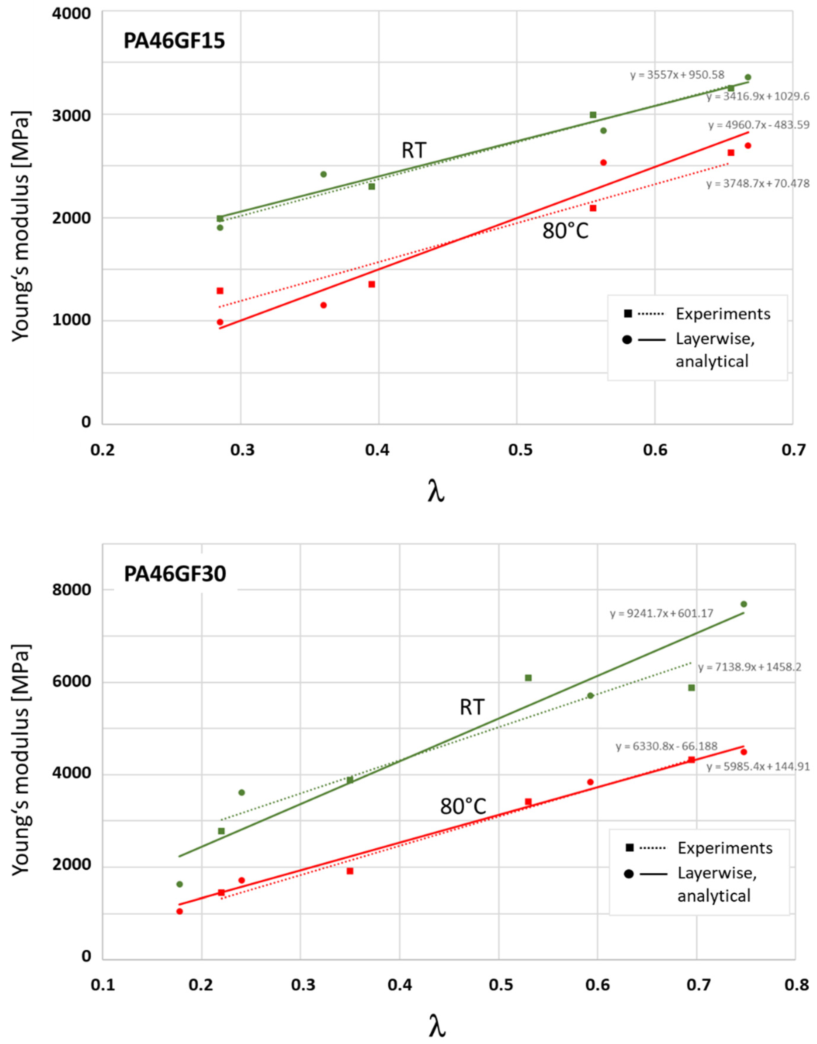
4.3. Analytical Results
5. Discussion
6. Conclusions
Author Contributions
Funding
Data Availability Statement
Acknowledgments
Conflicts of Interest
References
- Price, C.D.; Hine, P.J.; Whiteside, B.; Cunha, A.M.; Ward, I.M. Modelling the elastic and thermoelastic properties of short fibre composites with anisotropic phases. Compos. Sci. Technol. 2006, 66, 69–79. [Google Scholar] [CrossRef]
- Lopez, D.; Thuillier, S.; Grohens, Y. Prediction of elastic anisotropic thermo-dependent properties of discontinuous fiber-reinforced composites. J. Compos. Mater. 2020, 54, 1913–1923. [Google Scholar] [CrossRef] [Green Version]
- Cosmi, F.; Bernasconi, A.; Sodini, N. Phase contrast micro-tomography and morphological analysis of a short carbon fibre reinforced polyamide. Compos. Sci. Technol. 2011, 71, 23–30. [Google Scholar] [CrossRef] [Green Version]
- Advani, S.G.; Tucker, C.L. The use of tensors to describe and predict fiber orientation in short fiber composites. J. Rheol. 1987, 31, 751–784. [Google Scholar] [CrossRef]
- Fu, S.-Y.; Lauke, B.; Mai, Y.W. Science and Engineering of Short Fibre-Reinforced Polymer Composites, 2nd ed.; Woodhead Publishing: Duxford, UK; Cambridge, MA, USA, 2019. [Google Scholar]
- Dean, A.; Grbic, N.; Rolfes, R.; Behrens, B. Macro-mechanical Modeling and Experimental Validation of Anisotropic, Pressure- and Temperature-dependent Behavior of Short Fiber Composites. Compos. Struct. 2019, 211, 630–643. [Google Scholar] [CrossRef]
- Bernasconi, A.; Cosmi, F.; Dreossi, D. Local anisotropy analysis of injection moulded fibre reinforced polymer composites. Compos. Sci. Technol. 2008, 68, 2574–2581. [Google Scholar] [CrossRef] [Green Version]
- Wang, J.; Cook, P.; Bakharev, A.; Costa, F.; Astbury, D. Prediction of Fiber Orientation in Injection-Molded Parts Using Three-Dimensional Simulations. AIP Conf. Proc. 2016, 1713, 040007. [Google Scholar] [CrossRef] [Green Version]
- Gruber, G.; Haimerl, A.; Wartzack, S. Consideration of orientation properties of Short Fiber Reinforced Polymers within Early Design Steps. FEA Inf. Eng. J. 2013, 2, 2163–2167. [Google Scholar]
- Nutini, M.; Vitali, M. Simulating anisotropy with Ls-dyna in glass-reinforced, polypropylene-based components. In Proceedings of the 9th LS-DYNA German Forum, Bamberg, Germany, 12–13 October 2010; p. 12. [Google Scholar]
- Bauer, C. Charakterisierung und Numerische Beschreibung des Nichtlinearen Werkstoff- und Lebensdauerverhaltens Eines Kurzglasfaserverstärkten Polymerwerkstoffes unter Berücksichtigung der im µCT Gemessenen Lokalen Faserorientierung; Als Manuskript Gedruckt; Institut für Verbundwerkstoffe GmbH: Kaiserslautern, Germany, 2017. [Google Scholar]
- Affdl, J.C.H.; Kardos, J.L. The Halpin-Tsai equations: A review. Polym. Eng. Sci. 1976, 16, 344–352. [Google Scholar] [CrossRef]
- Kalaprasad, G.; Joseph, K.; Thomas, S.; Pavithran, C. Theoretical modelling of tensile properties of short sisal fibre-reinforced low-density polyethylene composites. J. Mater. Sci. 1997, 32, 4261–4267. [Google Scholar] [CrossRef]
- Brunbauer, J.; Mösenbacher, A.; Guster, C.; Pinter, G. Fundamental influences on quasistatic and cyclic material behavior of short glass fiber reinforced polyamide illustrated on microscopic scale. J. Appl. Polym. Sci. 2014, 131, 1–14. [Google Scholar] [CrossRef]
- Mortazavian, S.; Fatemi, A. Effects of fiber orientation and anisotropy on tensile strength and elastic modulus of short fiber reinforced polymer composites. Compos. Part B Eng. 2015, 72, 116–129. [Google Scholar] [CrossRef]
- De Monte, M.; Moosbrugger, E.; Quaresimin, M. Influence of temperature and thickness on the off-axis behaviour of short glass fibre reinforced polyamide 6.6—Quasi-static loading. Compos. Part. Appl. Sci. Manuf. 2010, 41, 859–871. [Google Scholar] [CrossRef]
- Stommel, M.; Stojek, M.; Korte, W. FEM zur Berechnung von Kunststoff- und Elastomerbauteilen; Hanser: München, Germany, 2011. [Google Scholar]
- Islam, M.A.; Begum, K. Prediction Models for the Elastic Modulus of Fiber-reinforced Polymer Composites: An Analysis. J. Sci. Res. 2011, 3, 225–238. [Google Scholar] [CrossRef]
- Zebdi, O.; Boukhili, R.; Trochu, F. An Inverse Approach Based on Laminate Theory to Calculate the Mechanical Properties of Braided Composites. J. Reinf. Plast. Compos. 2009, 28, 2911–2930. [Google Scholar] [CrossRef]
- Esha, E.; Hausmann, J. Development of an Analytical Model to Predict Stress–Strain Curves of Short Fiber-Reinforced Polymers with Six Independent Parameters. J. Compos. Sci. 2022, 6, 140. [Google Scholar] [CrossRef]
- Jones, R.M. Mechanics of Composite Materials, 2nd ed.; Taylor & Francis: Philadelphia, PA, USA, 1999. [Google Scholar]
- Aircraft Engineering and Aerospace Technology. Guideline VDI. 2014 Part 3: Development of Fibre Reinforced Plastics Components, Analysis. Aircr. Eng. Aerosp. Technol. 2007, 79, 1–159. [Google Scholar] [CrossRef]


| Temperature | Orientation | Thickness [mm] | Young’s Modulus [MPa] | Tensile Strength [MPa] | Strain at Break [%] |
|---|---|---|---|---|---|
| RT | 0° | 2 | 3249 ± 36 | 87.4 ± 1.1 | 14.34 ± 1.42 |
| 3 | 2992 ± 67 | 83.3 ± 0.6 | 15.16 ± 0.64 | ||
| 90° | 2 | 1988 ± 79 | 69.4 ± 0.4 | 21.09 ± 2.0 | |
| 3 | 2296 ± 77 | 74.0 ± 0.7 | 17.88 ± 1.49 | ||
| 80 °C | 0° | 2 | 2627 ± 238 | 72.5 ± 1.2 | 13.69 ± 1.19 |
| 3 | 2092 ± 137 | 69.9 ± 7.7 | 14.06 ± 0.56 | ||
| 90° | 2 | 1292 ± 69 | 49.8 ± 1.0 | 22.86 ± 2.11 | |
| 3 | 1356 ± 55 | 53.1 ± 0.2 | 20.39 ± 0.97 |
| Fiber Content | 15% | 30% | ||
|---|---|---|---|---|
| Temperature | RT | 80 °C | RT | 80 °C |
| Em | 2631 | 1842 | 4662 | 2775 |
| Ea,core | 212 | 691 | 1051 | 1064 |
| Ea,shell | 727 | 852 | 3026 | 1723 |
| E1,core | 2843 | 2533 | 5712 | 3838 |
| E1,shell | 3358 | 2694 | 7688 | 4498 |
| E2,core | 2420 | 1151 | 3611 | 1711 |
| E2,shell | 1905 | 990 | 1636 | 1052 |
Publisher’s Note: MDPI stays neutral with regard to jurisdictional claims in published maps and institutional affiliations. |
© 2022 by the authors. Licensee MDPI, Basel, Switzerland. This article is an open access article distributed under the terms and conditions of the Creative Commons Attribution (CC BY) license (https://creativecommons.org/licenses/by/4.0/).
Share and Cite
Hausmann, J.; Esha; Schmidt, S.; Krummenacker, J. Mean Value-Amplitude Method for the Determination of Anisotropic Mechanical Properties of Short Fiber Reinforced Thermoplastics. J. Compos. Sci. 2022, 6, 179. https://doi.org/10.3390/jcs6060179
Hausmann J, Esha, Schmidt S, Krummenacker J. Mean Value-Amplitude Method for the Determination of Anisotropic Mechanical Properties of Short Fiber Reinforced Thermoplastics. Journal of Composites Science. 2022; 6(6):179. https://doi.org/10.3390/jcs6060179
Chicago/Turabian StyleHausmann, Joachim, Esha, Stefan Schmidt, and Janna Krummenacker. 2022. "Mean Value-Amplitude Method for the Determination of Anisotropic Mechanical Properties of Short Fiber Reinforced Thermoplastics" Journal of Composites Science 6, no. 6: 179. https://doi.org/10.3390/jcs6060179
APA StyleHausmann, J., Esha, Schmidt, S., & Krummenacker, J. (2022). Mean Value-Amplitude Method for the Determination of Anisotropic Mechanical Properties of Short Fiber Reinforced Thermoplastics. Journal of Composites Science, 6(6), 179. https://doi.org/10.3390/jcs6060179