5.1. Agglomeration of CNTs
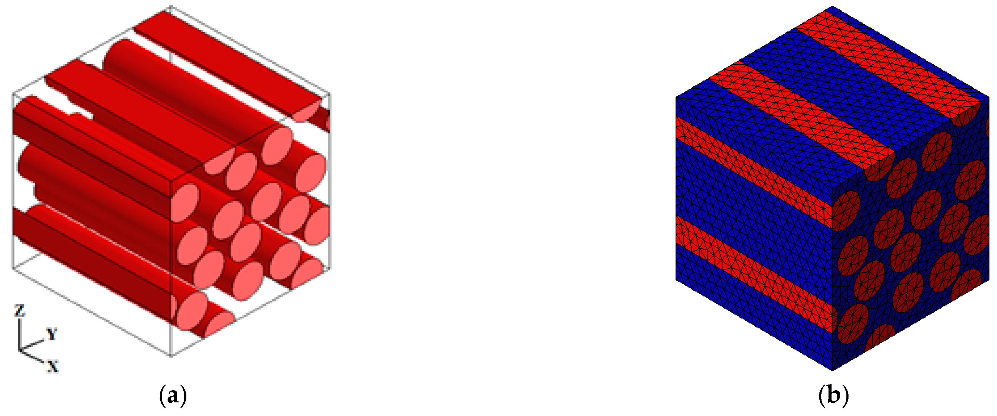
First, the nanosized reinforcing phase is apt to agglomerate, causing a spatially non-uniform distribution of the fillers in composites. To theoretically examine the agglomeration effect, we assumed that some graphene sheets are concentrated in some spherical regions in the matrix, while the rest keep a desired uniform dispersion, as illustrated in
Figure 11. Then, the composite was divided into two parts with different loadings of reinforcement which can be considered as two different phases in calculation. We gave the names agglomeration phase and effective matrix phase to the regions inside and outside the spheres, respectively, and further recommend that in both phases the graphene sheets are randomly oriented. In our model, a two-parameter description was employed to characterize such a special distribution [
23], where the agglomeration parameters are written as
If
denotes the total volume of CNTs inserted in the matrix, it can be defined as the sum of two contributes
In which
and
represent the volume of nanofillers within the inclusions and scattered in the matrix, respectively. Thus, the total volume W of a representative element is given by the following relation
where
stands for the matrix volume.
The volume fraction of CNTs
and of the matrix
can be expressed as follows
In which the relation
+
= 1 allows to relate these two quantities. The reinforcing phase
can be seen as the sum of the volume fraction of CNT within the inclusions
and the volume fraction of the nanoparticles scattered in the matrix
as shown below
Then the volume fraction of nanofillers in the agglomeration phase
and that in the effective matrix phase
can be formulated as
A two-step procedure was applied to reckon the above model. First, the overall elastic properties of the agglomeration and the effective matrix phases are calculated from Equations (80) and (85) by replacing
with
and
given in Equation (84), respectively. The bulk modulus of the spherical inclusions
, and the effective matrix
are computed as
Whereas the corresponding shear modulus of the spherical inclusions
, and the effective matrix
are computed as
It should be pointed out that
and
specify the bulk and the shear moduli of the sole isotropic matrix, can be formulated from Equation (90). For the elastic Hill’s moduli, CNT inclusions are computed from Equations (3)–(6).
Secondly, the agglomeration phase is considered as spherical inclusions embedded in the effective matrix. The effective bulk moduli
and shear moduli
of this hybrid matrix, enriched by CNTs or GNP both included in the spherical inclusions and scattered in the matrix can be computed as
In which
stands for the Poisson’s ratio defined as follows
The hybrid matrix is evidently isotropic. Therefore, the Young’s modulus , the Poisson’s ratio and the density are required to define its properties. They can be computed from Equations (9)–(10), respectively
For , with The first parameter μ defines the width of the spherical inclusion with respect to the total volume W. On the other hand, the second agglomeration parameter η quantifies the volume of CNTs inside the inclusions with respect to total volume of CNTs . In general, three limit cases of the agglomeration ratio can be defined depending on the values of .
For
and
th, the agglomeration is partial, and the nanofibers are both included in the inclusions and scattered in the matrix (
Figure 11b). It should be noted that the heterogeneity of CNTs is amplified for
, by increasing the value of the parameter η. In contrast, if
is set, the volume of CNTs is completely concentrated in the inclusions
, which coincide with the whole reference domain (
). This circumstance is depicted in
Figure 11a and represents a null level of agglomeration. Finally, the complete agglomeration of CNTs is defined by
and
(
Figure 11c). In other words, all the CNTs are located within the spherical inclusions.
5.1.1. Method Comparison
Before studying the agglomeration effect using Shi’s model [
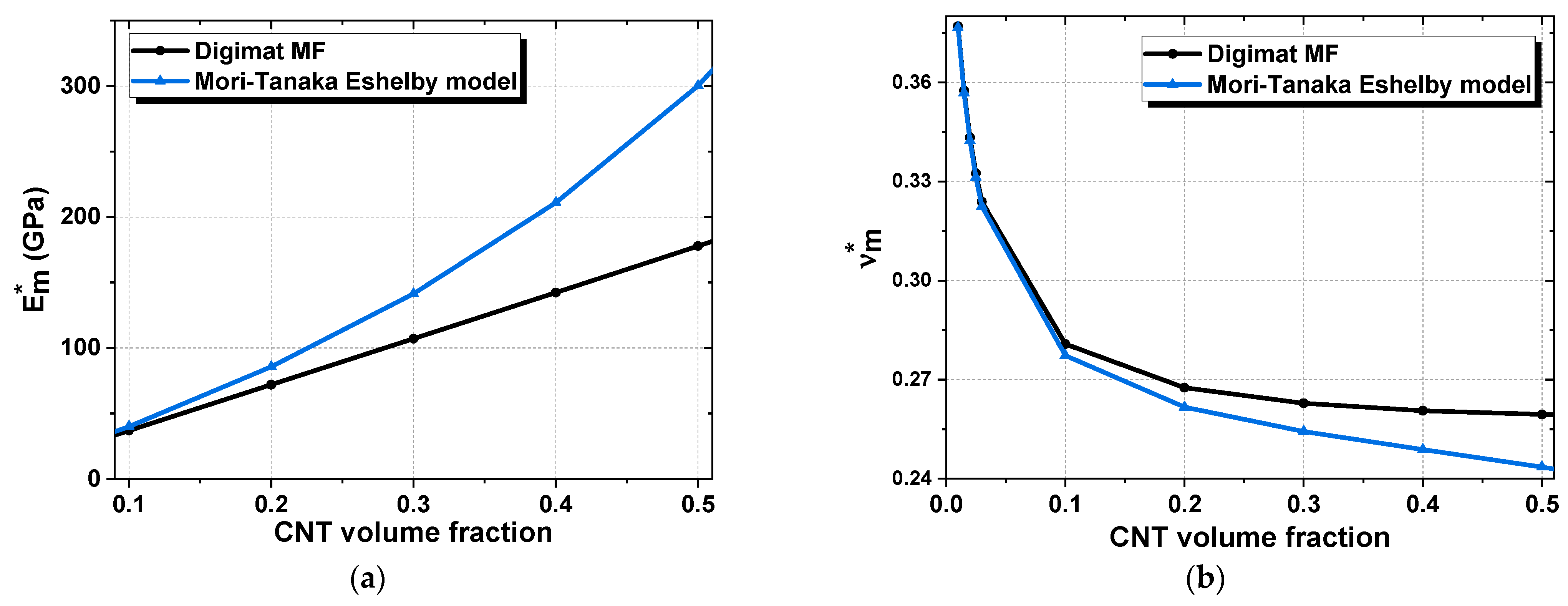
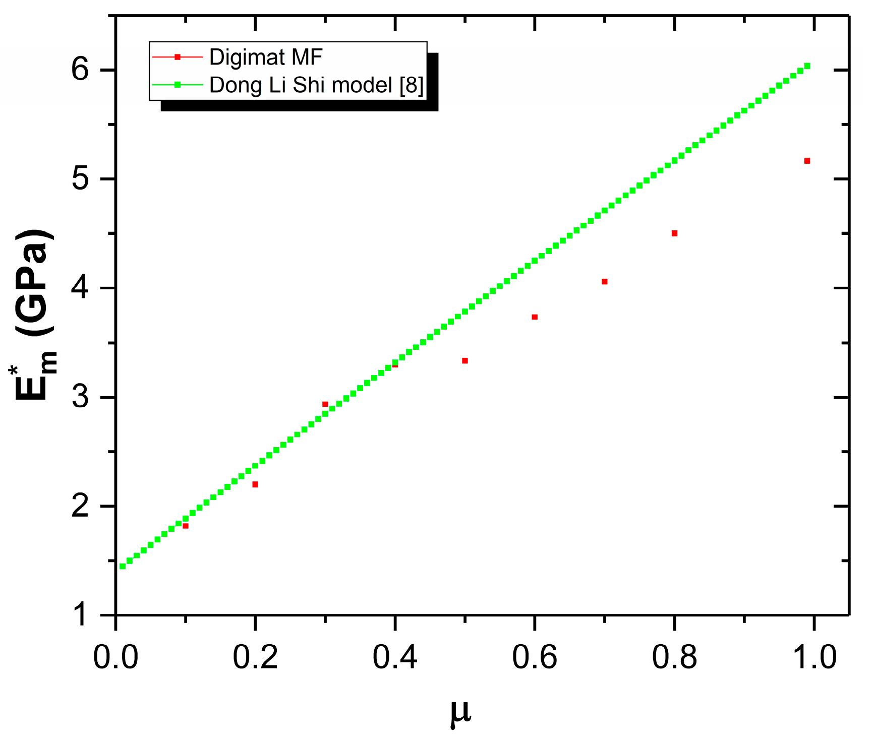
22], we investigated the validity of the model by comparing results from the analytical model (
Table 6) with semi-numerical results from Digimat MF.
It was supposed that the inclusions had a prolate ellipsoid with an aspect ratio of 104, and the agglomeration to have a spherical shape. The volume fraction of CNTs was assumed to be equal to 1%.
As seen in
Figure 12, there is an acceptable agreement between the two approaches: until
, the results from Digimat MF tend to be linear. The errors between the two approaches can be explained by several explanations: errors can come from the fact that inclusions in the analytical model are assumed to have an infinite aspect ratio, in addition the low value of
used in this study plays a role in the validity of this comparison as when we increased the latter parameter, agreement was no longer found.
5.1.2. Results and Discussions
The influences of the parameters
and
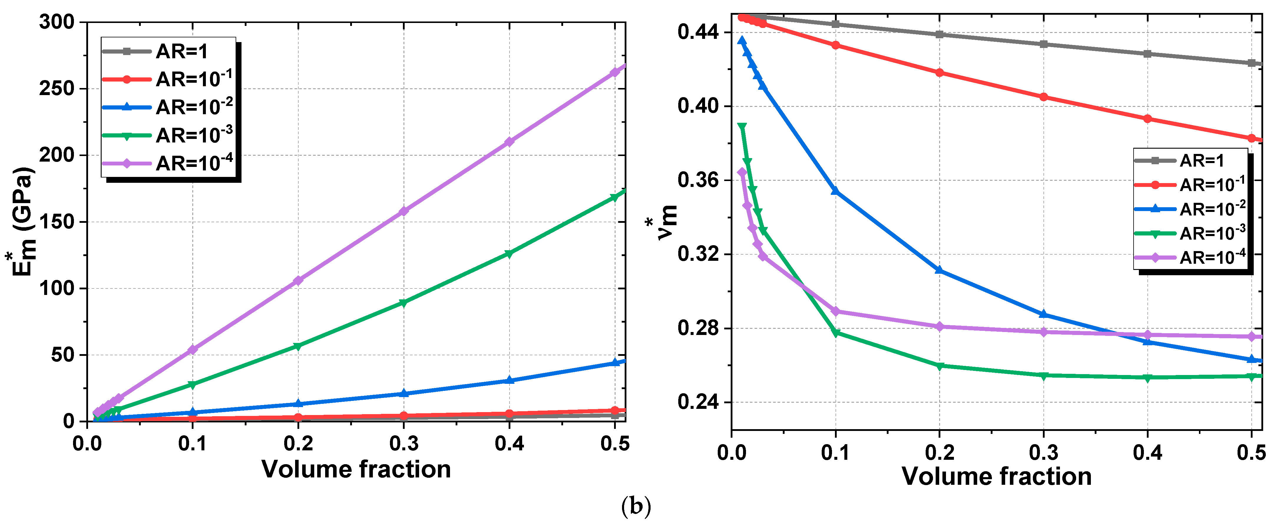
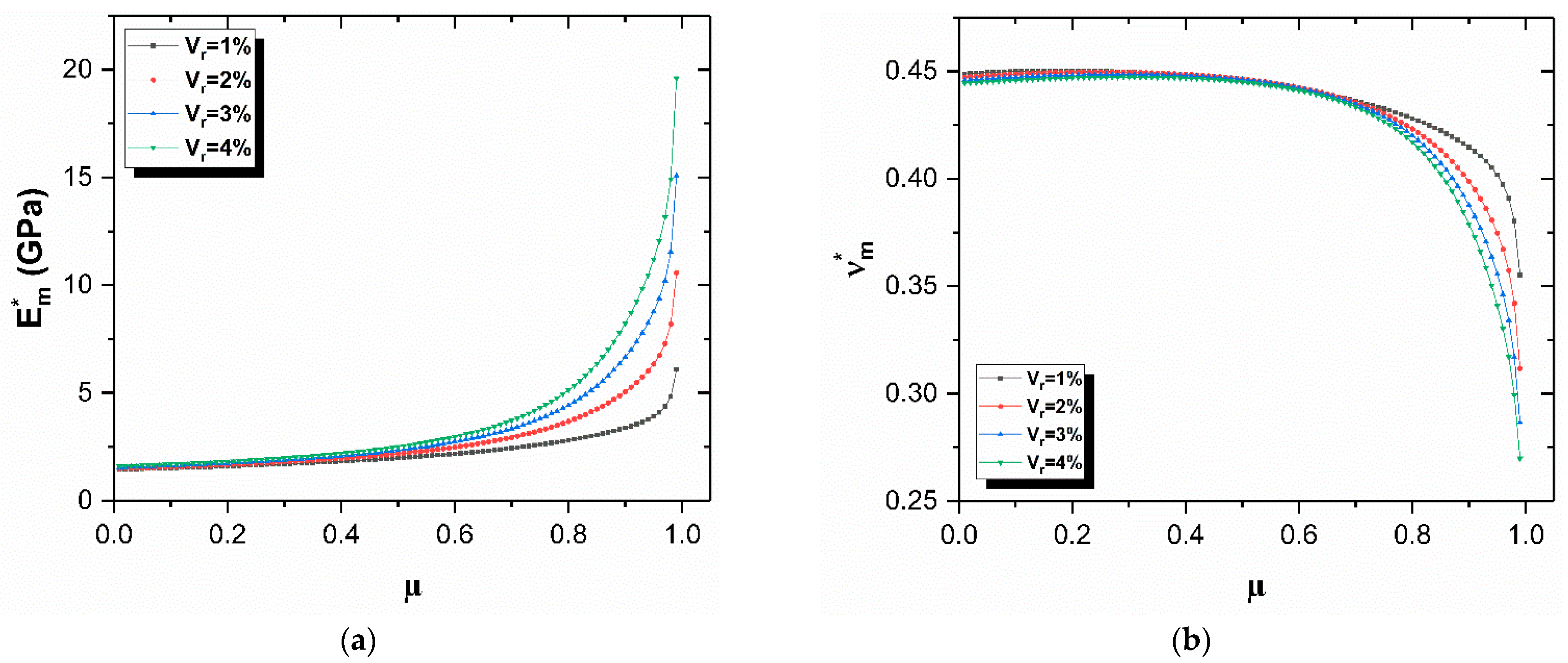
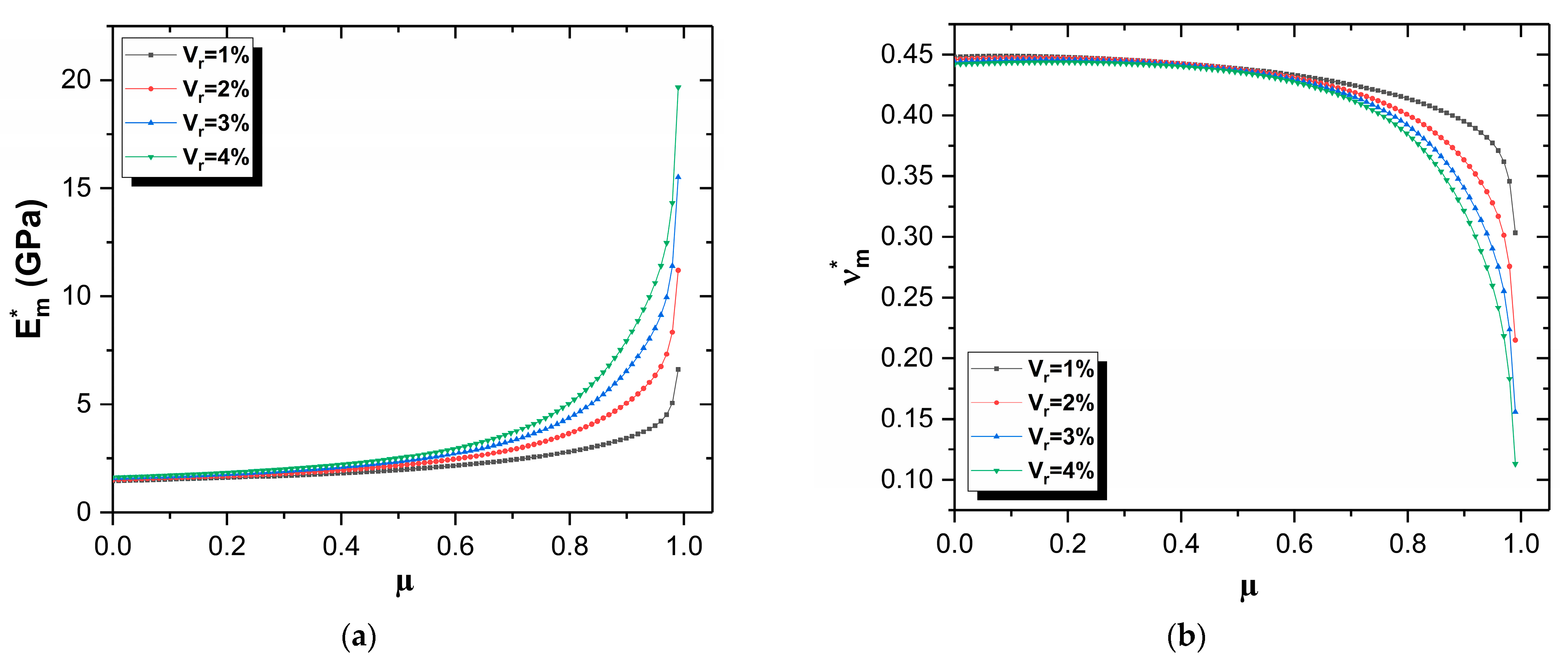
on the effective modulus were investigated individually by fixing another for only a small volume fraction, as in reality the use of nanofillers is limited to low levels. First, we considered the most severe case of agglomeration where all the inclusions were concentrated in the same place which we can express mathematically by
. We plotted the effective Young’s modulus and Poisson’s ratio under different volume fractions in function of
(
Figure 13).
The effective elastic modulus has a maximum value when the CNTs are uniformly distributed in the composite. As the agglomeration parameter decreases, the effective stiffness also decreases rapidly. It is also noted that for ≤ 0.6, the addition of CNTs has no effect on the elastic properties of the reinforced polymer. Both agglomeration parameters are required to describe this phenomenon. The first η indicates the amount of inclusions located in the agglomeration and the other indicates the size of the agglomerations.
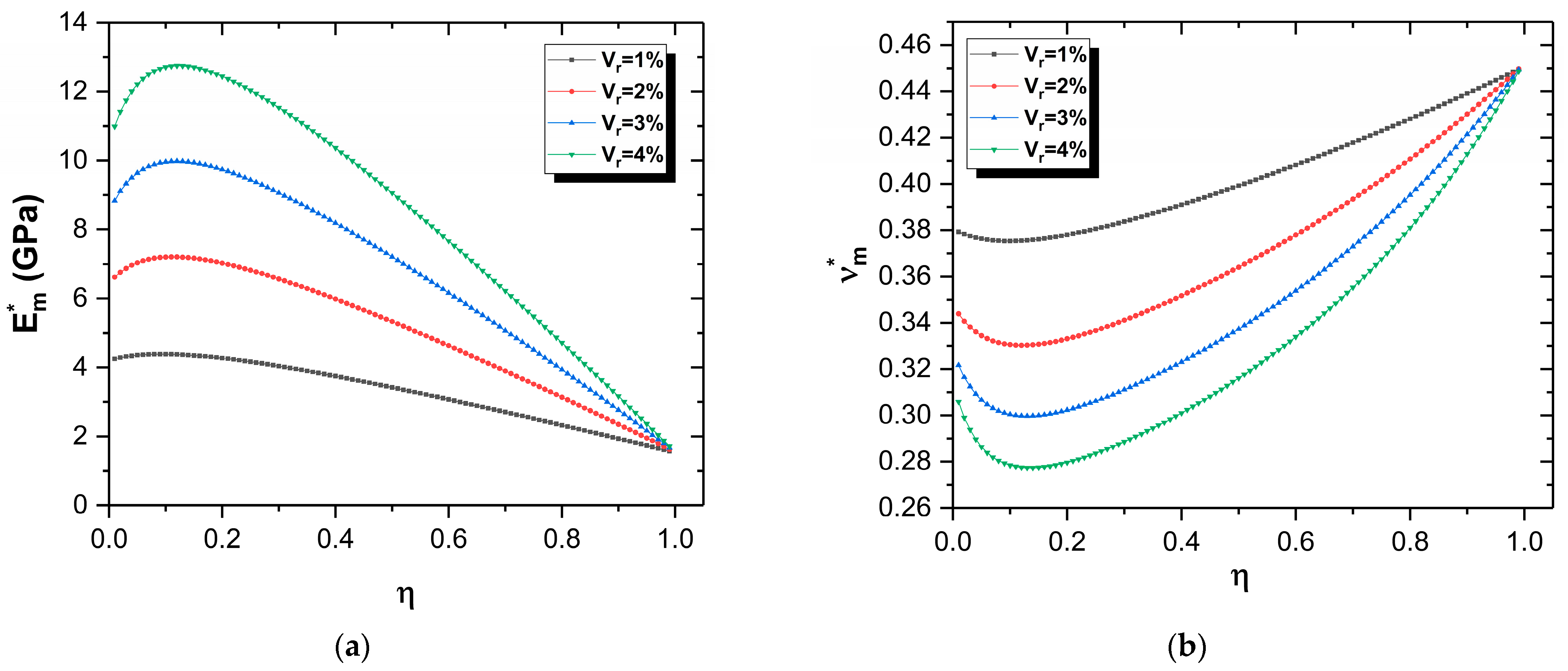
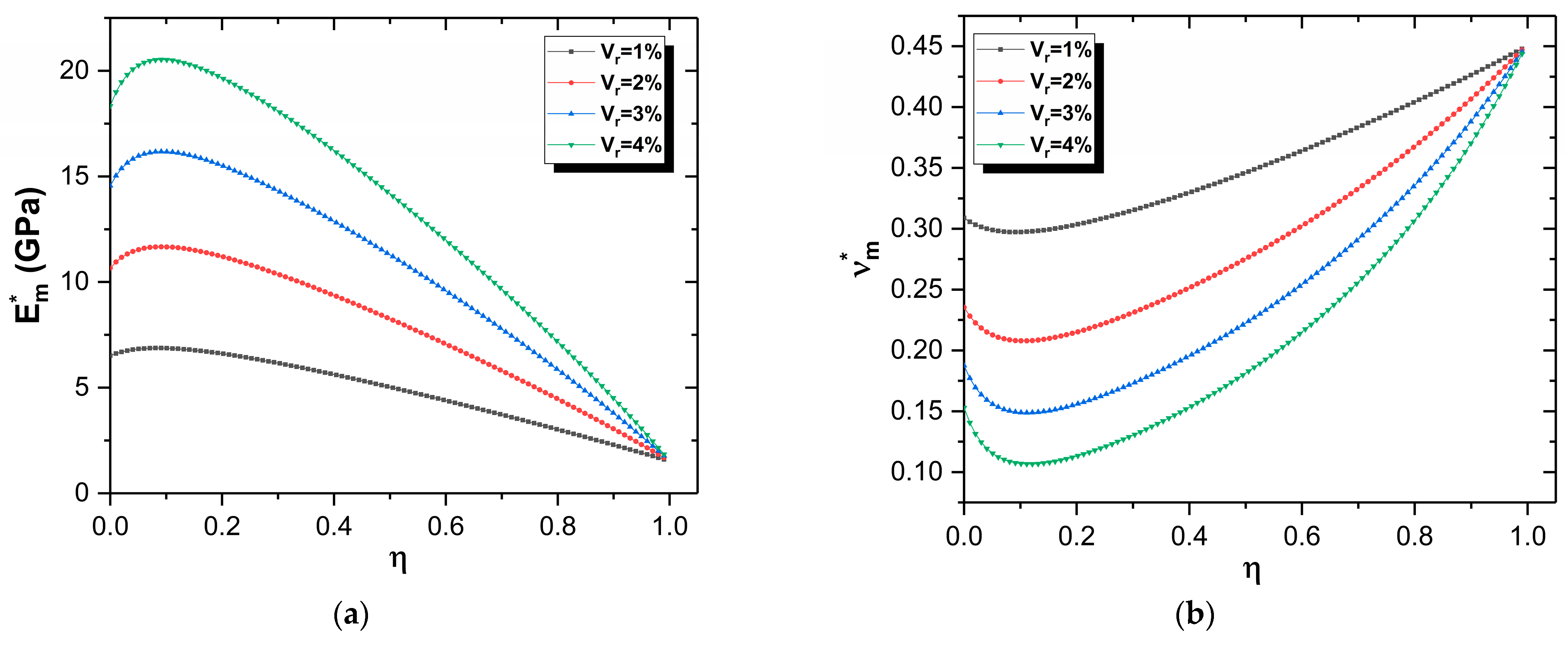
The effective properties are shown in
Figure 14 for
= 0.2, where it is seen that with the increase of the relative amount of CNTs in the concentrated regions, the effective Young’s modulus increases slightly to a maximum value of 20 GPa for a volume fraction of 4% and
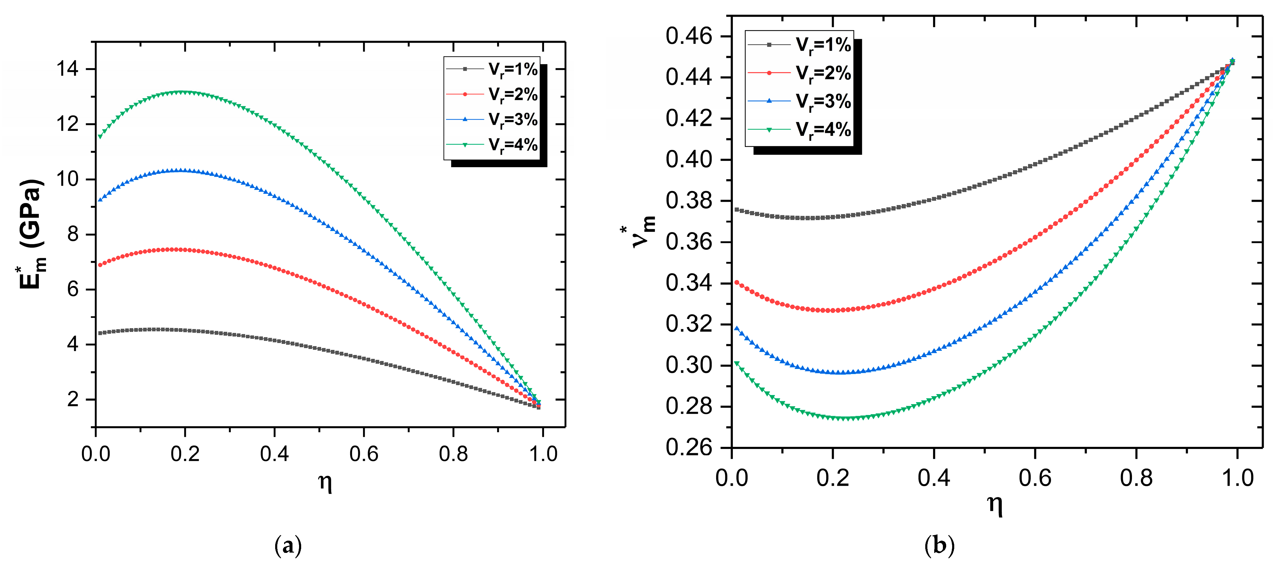
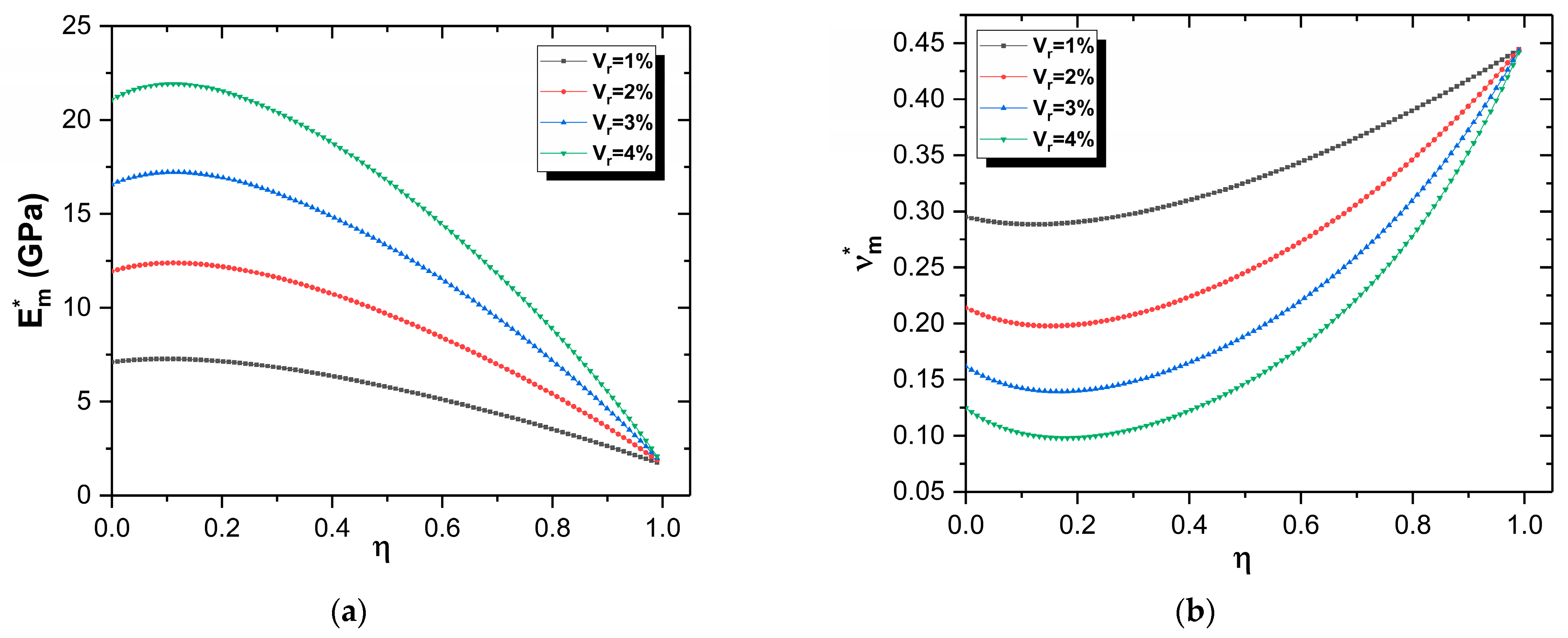
= 0.15 before dropping sharply to reach its minimum value when η reaches the unity. For
= 0.5 (
Figure 15), we can observe that the curves keep the similar tendency but with greater magnitudes, so it can be concluded that increasing the volume of the concentrated regions leads to an increase in the effective properties.


 ,
, 


