1. Introduction
Butterflies are insects in the macrolepidopteran clade Rhopalocera from the order Lepidoptera, in which moths are also included. Adult butterflies have large, often brightly coloured wings, and conspicuous, fluttering flight. Their colors and markings not only can protect them from predators but also are essential features for researchers and people who are interested in butterflies to recognize their categories. However, it is arduous to classify butterflies based on their patterns, because some features, such as shapes, wing colors, and venations, are complicated to distinguish [
1]. Traditional butterfly identification techniques, such as the use of taxonomic keys [
2], depend on manually identifying and classifying by highly trained individuals, which follow the same methodology with various more modern methods such as DNA sequencing [
3]. Currently, researchers from around the world rely mostly on rather time-consuming processes that are inefficient in dealing with the distribution and diversity of butterflies. Besides, taxonomic approaches are made difficult in practice due to the lack of adequate reference collection and professional knowledge [
4,
5,
6,
7,
8]. Therefore, to tackle the so-called “taxonomy crisis” [
9], the academic community calls for modern and automated technologies in dealing with species identification.
In the image classification field, traditional machine learning algorithms, such as K-Nearest Neighbor (KNN) and Support Vector Machine (SVM), are widely adopted to solve classification problems and especially perform well on small datasets. However, when addressing a large dataset with more complicated features and classes, deep learning outweighs traditional machine learning. Recently, transfer learning is more prevalent than ever before, because it can save a large amount of computing and time resources to develop deep networks from the very beginning. Pre-trained deep learning models can be the starting point for dealing with related problems. Because classification targets, such as butterflies, have too many categories and some of their features are similar so that machine learning and deep learning will be handy to assist researchers to classify the confusing targets.
Because of the prevailing of smartphones, today both mobile phone users and the artificial intelligence industry expect to have systems implemented in mobile applications to achieve convenience. The previous widely used method to classify images through mobile devices (still being used under certain circumstances) was to save the model on a server. The targets and results are transferred between the server and mobile devices. and this causes latency due to bilateral communication between the server and mobile devices and insecurity of privacy. Now TensorFlow Mobile and its updated version TensorFlow Lite can solve these problems. They can transform deep learning models to a specifically optimized format and transplant them into mobile applications so that considerable computational power of the mobile hardware can be saved when tasks are running. As a result, researchers can use smartphones to classify targets such as butterflies both indoor or outdoor, especially when they are doing field study without any connection to the network but hope to know the categories immediately.
This paper aimed to build four models and develop an Android application as a butterfly detector. After model selection, the most effective one was implemented in an Android application to build a system to detect butterfly categories.
2. Related Works
In the traditional machine learning area, SVM [
10] is one of the most effective methods to address various kinds of problems such as classification and regression. Recently, the Principal Component Analysis (PCA) [
11] algorithm combined with SVM is also prevailing since this method can enhance the efficiency of training the model to a large extent. Reference [
12] adopted PCA and SVM on two face datasets called AT&T face database and Indian face database (IFD), and reached an accuracy of 90.24% and 66.8% on each dataset. Reference [
13] used this method to detect the event that people fall on the floor and had an accuracy of 82.7%. In 2016, Reference [
14] applied PCA and multi-kernel SVM to compare healthy controls and Alzheimer’s Disease patients with their brain region of interest, and finally achieved an accuracy of 84%.
As tasks are getting more complicated than ever before, the volume of datasets has increased to a size which cannot be solved by traditional machine learning methods. As a result, the role of artificial neural networks is revealed. Reference [
15] developed a neural network structure intending to classify a dataset including 740 species and 11,198 samples. They had a 91.65% accuracy with fish, 92.87% and 93.25% of plants and butterflies, respectively.
In the specific field of butterfly detection, Reference [
16] proposed Content-Based Image Retrieval (CBIR) to detect butterfly species, but the total accuracy is 32% for the first match and 53% for the first three matches. Reference [
17] applied Extreme Learning Machine (ELM) to classify butterflies and compared the results with the SVM method. The ELM method has an accuracy of 91.37%, which is slightly higher than the SVM. Reference [
18] built a single neural network to classify butterflies according to their shapes of wings, and the accuracy is 80.3%. Reference [
19] is research aiming to classify all butterfly species in China, which adopted three methods: Zero Forcing (ZF), Visual Geometry Group (VGG)_Convolution Neural Network (CNN) and VGG16, to compare the performance. The results showed that ZF has an accuracy of 59.8%, while VGG_CNN and VGG16 had 64.5% and 72.8%, respectively.
As for transfer learning, Reference [
20] used the DeepX toolkit (DXTK), which includes several pre-trained low-resource deep learning models, to integrate models in mobile devices. Reference [
21] used a multi-task, part-based Deep CNN (DCNN) structure for feature detection, and evaluated its performance, then deployed the structure on a mobile device. Reference [
22] built real-time CNN networks based on transfer learning to detect the regions where have Post-it
, and transformed these models to the format which can be used on smartphones with TensorFlow Lite tools. A Faster Region CNN (RCNN) ResNet50 architecture achieved the highest mAP (mean Average Precision), which is 99.33% but the inference time is 20018 milliseconds (ms).
The difference in the accuracy of traditional machine learning, deep learning and transfer learning methodologies on butterfly detection has not been the focus of any research so far and a mobile application to detect butterfly has never been developed. Therefore, in this paper, after optimized certain parameters, not only we improved the accuracy from previous studies with deep learning models, but we also created a practical Android application that has a relatively short inference time.
3. Methodologies
From each field of traditional machine learning, deep learning and transfer learning, one or two techniques were adopted to build a model for butterfly classification.
3.1. Traditional Machine Learning
3.1.1. Support Vector Machine (SVM)
SVM is one of the most important classical machine learning algorithms. It was first proposed by Cortes and Vapnik in 1995 [
10]. It has a lot of outstanding superiority in addressing small scale, nonlinear, and high-dimensional pattern recognition problems. SVM is a two-class classification model based on the VC (Vapnik–Chervonenkis) dimension theory and structural risk minimization principle of statistical learning theory. A linear classifier with the largest interval in the feature space is the definition of the SVM algorithm. Its objective is to determine the maximum interval. Then the problem is transformed into a convex quadratic programming problem, and the maximum interval is the solution to this problem. However, our task is to complete a ten-class high-dimensional classification, which cannot be achieved by linear classifier, we applied nonlinear SVM with Radial Basis Function (RBF) kernel, which is also known as Gaussian kernel:
Generally speaking, a kernel can be interpreted as a similar shape function between two samples. The exponent range in the Gaussian kernel is , so the Gaussian kernel range . In particular, the value is 1 when the two samples are identical, and the value is 0 when the two samples are completely different.
The target of classifying a given data
is to determine a function
which can classify patterns of the input data accurately, in which
is a n-dimensional vector and
is its label [
23]. The hyperplanes can be expressed by
;
and the data can be separated linearly, if such a hyperplane exists. Hyperplane margins (
) have to be maximized to look for the optimum hyperplane. Lagrange multipliers (
) are applied to tackle this task [
24]. The decision function can be formulated as:
SVM can also address nonlinear classification problems by mapping the input vectors to a higher-dimensional space with kernel functions
[
25]. Therefore, the decision function can be expressed as:
Four commonly used kernel functions:
Linear:
Polynomial:
Radial Basis Function:
Sigmoid:
PCA was introduced to extract the most useful features in each image. PCA has a wide variety of applications in areas such as data compression to eliminate redundancy and data noise. Specifically, if the dataset is n-dimensional and there are m samples , PCA can reduce the dimensions of these m samples from n-dimensional to -dimensional, and the m -dimensional samples can represent the original dataset as much as possible. There would be a loss in the data from n-dimensional to -dimensional, but we wanted the loss to be as small as possible. The algorithm of PCA is demonstrated in the steps listed below.
Implimentation of the PCA Algorithm:
Supposing there are m n-dimensional samples and arraying the original data by columns into a matrix X with n rows and m columns;
Zero-averaging each row of X (representing an attribute field), i.e., subtracting the mean of the row;
Calculating the covariance matrix ;
Determining the eigenvalues of the covariance matrix and the corresponding eigenvectors;
Arranging the feature vectors decreasingly according to the corresponding feature value and selecting the first rows to form a matrix P;
is the new data after reducing to dimension.
Integrating PCA with SVM is widely adopted in pattern recognition as it not only can avoid the SVM kernel gram to become overlarge but also improves computational efficiency for classification [
26]. Therefore, we selected PCA/SVM method as one of the approaches to address this butterfly classification problem in this paper.
3.1.2. Decision Tree and Random Forests
A decision tree is a tree-like structure (binary tree or non-binary tree) that solves classification and regression problems by splitting samples into sub-populations recursively [
27]. Each of a decision tree’s non-leaf nodes represents a test on a feature attribute, each branch represents the output of this feature attribute over a range and each leaf node is a class. The process to use a decision tree is to start from the root node and test the feature attributes in samples, then select the branch according to the output until reach the leaf node. At last, the class of the leaf node is the decision result.
In 2001, Breiman and Cutler developed an algorithm to randomly ensemble decision trees into a forest [
28]. In the forest, there are many decision trees and all of these trees have no correlation and dependency between each other. After obtaining the forest, each decision tree in the forest will calculate the class of a new incoming sample (for the classification problems). The final decision depends on which class is voted by most trees. Random forests can tackle both discrete values, such as the Iterative Dichotomiser 3 (ID3) algorithm [
29], and continuous values, such as the C4.5 algorithm [
30]. Additionally, random forests can be used for unsupervised learning clustering and outlier detection. Because random forests are not sensitive to multicollinearity, they are robust to missing and unbalanced data so that they can predict well for up to thousands of variables [
28]. Random forests currently is one of the most prevalent methods for classification and regression problems in machine learning field.
Implimentation of the Random Forests (RF) Algorithm:
Take a random sample of size N with replacement from the data;
Take a random sample without replacement of the predictors;
Construct the first Classification And Regression Tree (CART) for partition of the data;
Repeat Step 2 for each subsequent split until the tree is as large as desired and do not prune;
Repeat Step 1 to Step 4 a large number of times (e.g., 500).
Random Forests is a great statistical learning model as it is highly efficient for the classification of multi-dimensional features and can realize feature selection. However, overfitting happens when data noise is relatively large.
3.2. Deep Learning
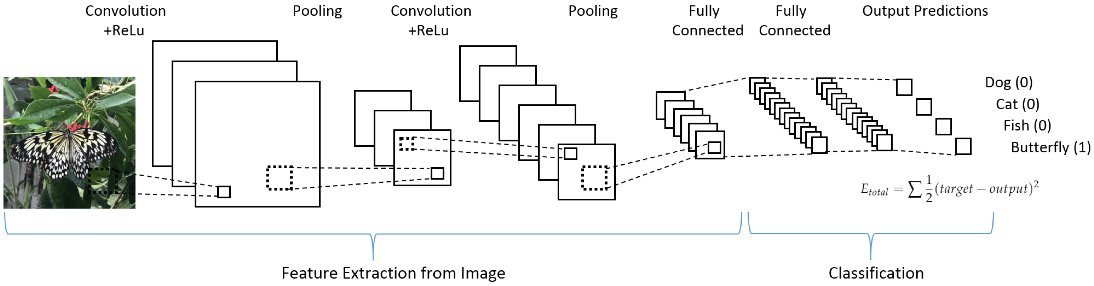
The most important advancement of deep learning over traditional machine learning is that its performance improves with the increasing of the amount of data. A 4 convolutional layers model (4-Conv CNN) was built from scratch for this paper. The structure of CNN is shown in
Figure 1. This 4-Conv CNN has 4 Conv2D layers, 2 MaxPooling layers, and 5 Dropout layers, and a fully connected layer is the following.
Functions of different layers:
The first layer in this structure is a Conv2D layer for the convolution operation which can extract features from the input data by sliding the filter over the input to generate a feature map. In this case, the size of the filter is .
The second layer is a MaxPooling2D layer for the max-pooling operation which can reduce the dimensionality of each feature. In this case, the size of the pooling window is .
The third layer is a Dropout layer for reducing overfitting. In this case, the dropout function will randomly abandon 20% of the outputs.
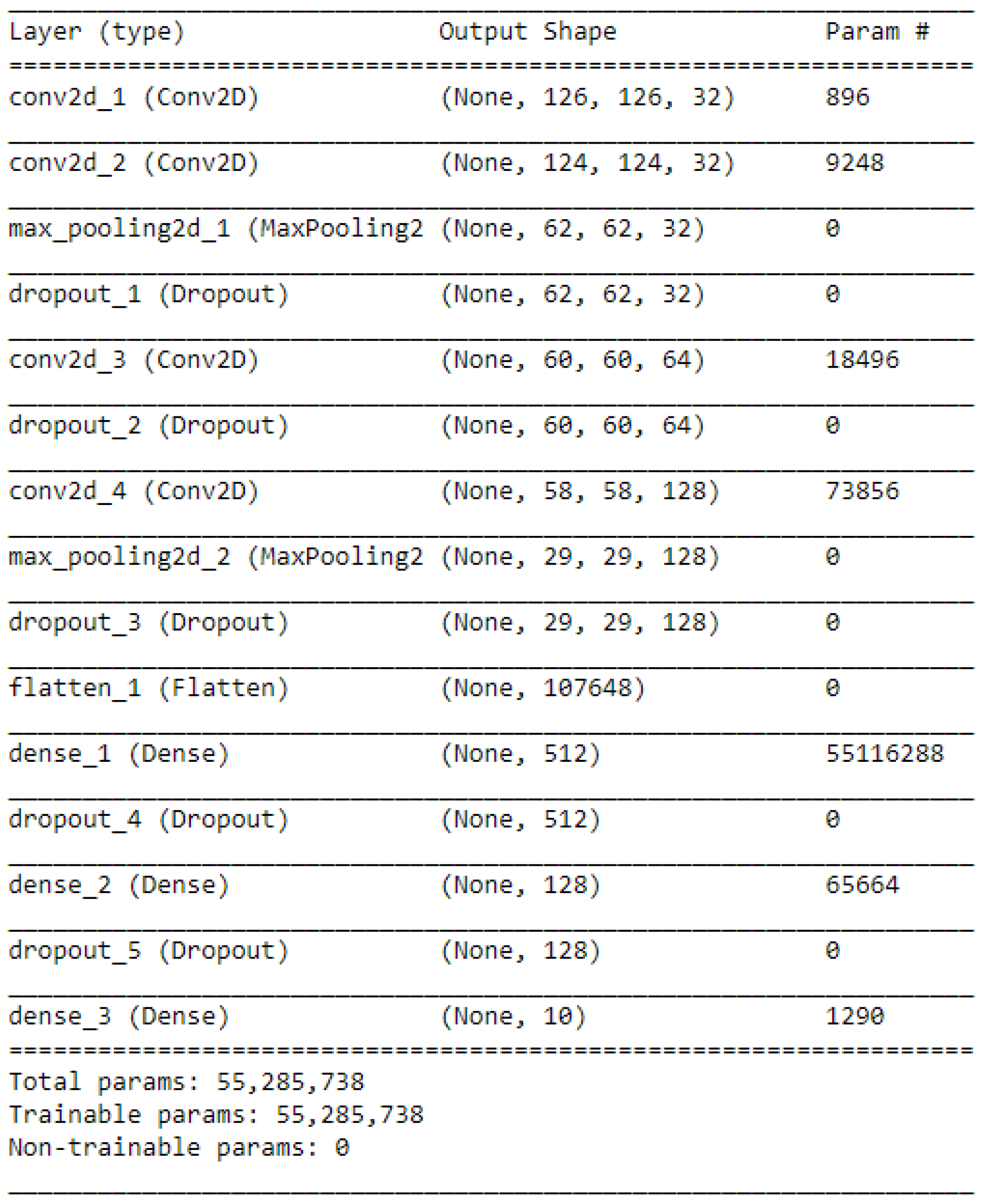
We repeated these steps to add more hidden layers, which are 4 Conv2D layers, 2 MaxPooling2D layers, and 5 Dropout layers. Then, a Flatten layer is used to flatten the output to 1D shape because the classifier will finally output a 1D prediction (category). Two Dense layers have a fully connected function and another Dropout layer between them can discard 30% of the outputs. Because this task is a 10 categories classification, a final layer is combined with a Softmax activation to transform the outputs to 10 possibilities. This is shown in
Figure 2.
3.3. Transfer Learning
As the name suggested, transfer learning migrates the learned parameters in a model to a new model to train the new model. Traditional machine learning and transfer learning are shown in
Figure 3. Considering that most of the data or tasks are related, already learned parameters in an existing model (pre-trained model) can be shared with the new model in some way through transfer learning, so as to accelerate and optimize the learning efficiency of the new model, and unlike most networks that need to start from scratch.
The last fully connected layer in a pre-trained model will be removed and two new fully connected layers will be added to the model when this model serves as a feature extractor. Except for these two new layers, all other structures and weights are fixed. Although we can also initialize all weights in the pre-trained model, it is not common to do so and it is suggested to have some of the earlier layers fixed because they stand for generic features.
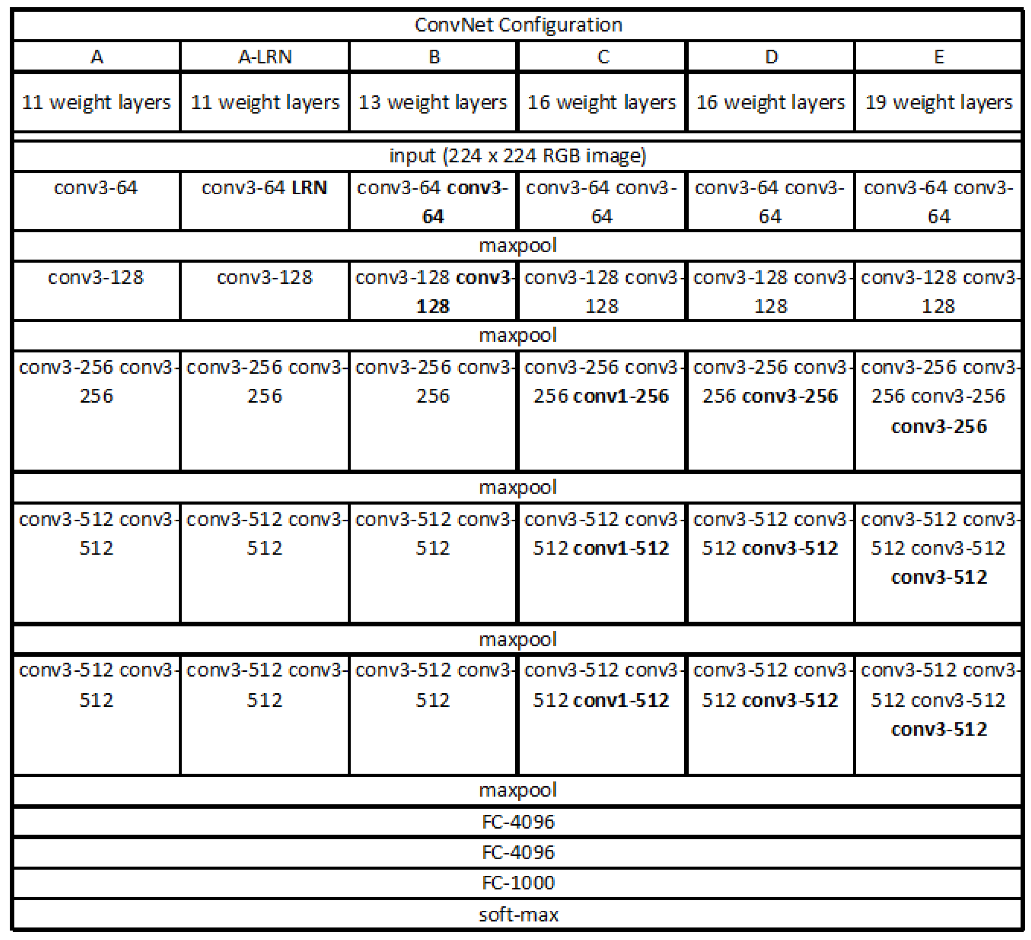
Recently, the advanced VGG19 [
31] is more widely used, shown in
Figure 4. One improvement of the VGG19 over other models is the use of several consecutive
convolution kernels instead of the larger convolution kernels. For a given receptive field (the local size of the input image related to the output), the use of stacked small convolution kernels is superior to the use of large convolution kernels, because multiple nonlinear layers can increase network depth to ensure more complex learning modes, and the cost is relatively small in terms of fewer parameters. As a result, we adopted the VGG19 as the base model for this paper. The convolutional base of VGG19 structure was frozen and we added our own fully connected layer on top of the base.
4. Dataset and Application
4.1. Dataset
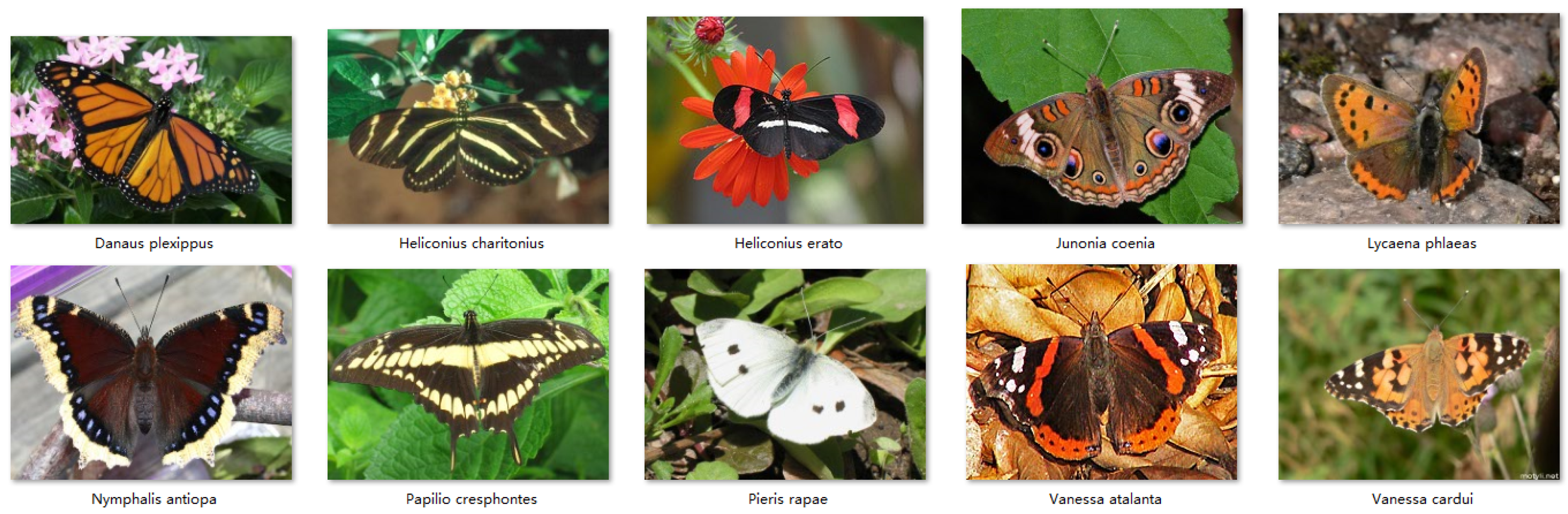
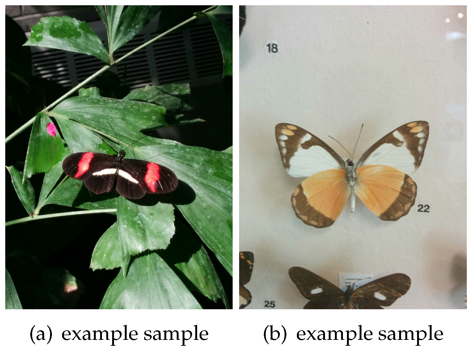
The dataset used in this project is called Leeds Butterfly Dataset [
32]. This dataset has ten species of butterflies with both images and textual descriptions. An example of the different categories is shown in
Figure 5. The origin of these images was gathered from Google Images according to the scientific name of the species.
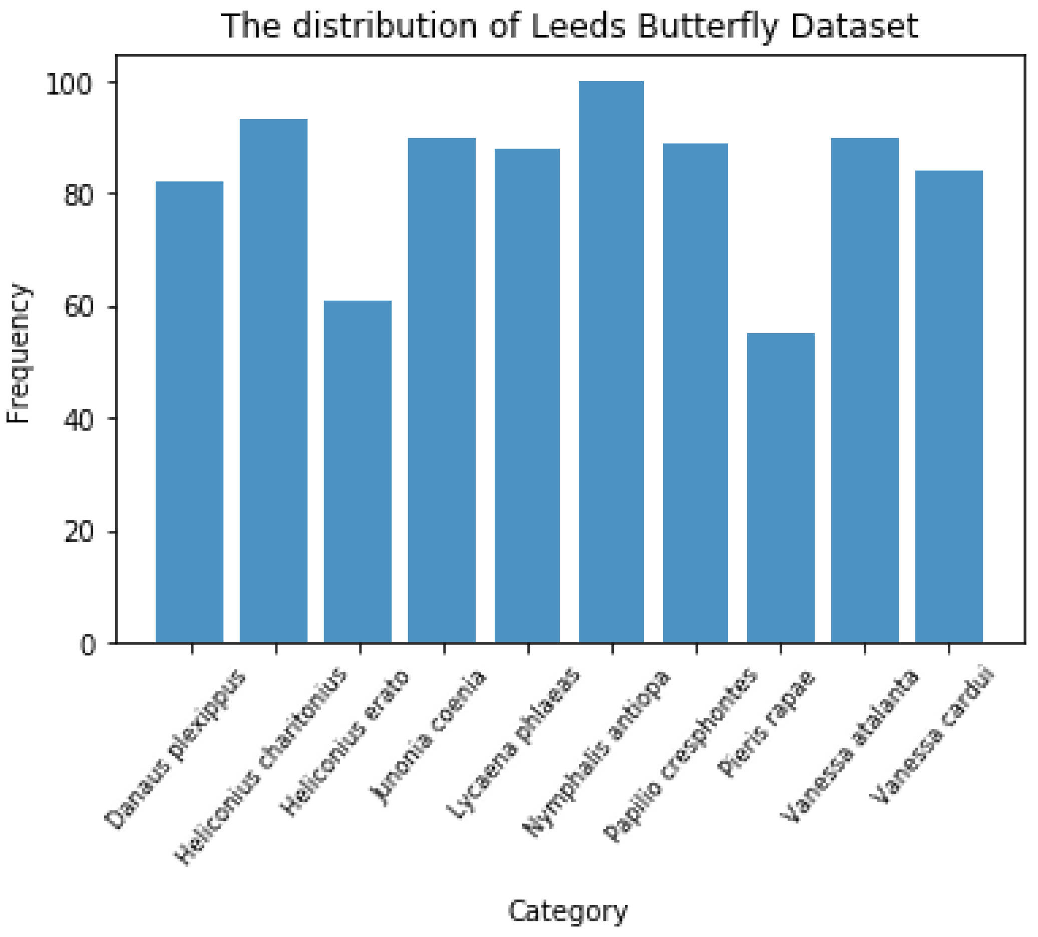
There are 832 images in total, and the image distribution of different species is relatively balanced, as shown in
Figure 6. This is beneficial for machine learning algorithms to learn the features of each category more evenly.
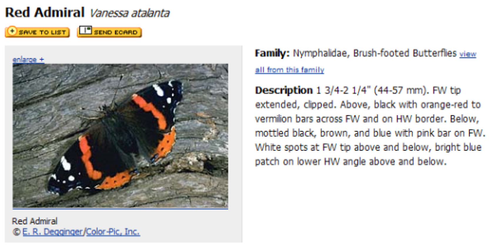
The textual descriptions of every butterfly species were collected from the eNature online nature guide [
33], which is for online open biology resources, shown in
Figure 7. The description files include the name, the normal size and a brief introduction of each species. The name was taken as the label of each image, and the brief introduction was used as a depiction in Android application when the system returns a prediction of what the user inputs.
4.2. Android Application
After model selection, we aimed to build an Android application (App) that used the best model to detect the category of the butterfly. We built the app in Android Studio. The Sdkversion of the environment is 27 and the mobile phone is API 19.
4.2.1. Comparison of Models Saved in Server and in Application
The traditional way to deploy deep learning models is to save the model on a server. When the client-side needs to have a prediction from the model, it should make a call to the server-side to get the result. After the data are processed on the server-side, the result will be sent back to the client-side and displayed. The server should respond to the requests as soon as possible. However, the server may produce slow work and there is also latency issue during data transmission. Additionally, users prefer not to send private data to servers because of the potential problems of cybersecurity. As a result, the demand for on-device intelligence capabilities is increasing. As a complement to the TensorFlow ecosystem, TensorFlow Mobile and TensorFlow Lite offer researchers and developers the opportunity to run deep learning models on smartphones and tablets locally with low latency, efficient runtimes, and accurate inference. Especially with the computational ability of GPU in presently used mobile devices, more complex deep learning models can take advantage of TensorFlow Lite, which allows massively parallelizable workloads and previously not available real-time applications to run fast enough on smartphones and tablets [
34]. Therefore, we chose to implement the model with the cutting-edge technology in this paper.
4.2.2. TensorFlow Mobile and TensorFlow Lite
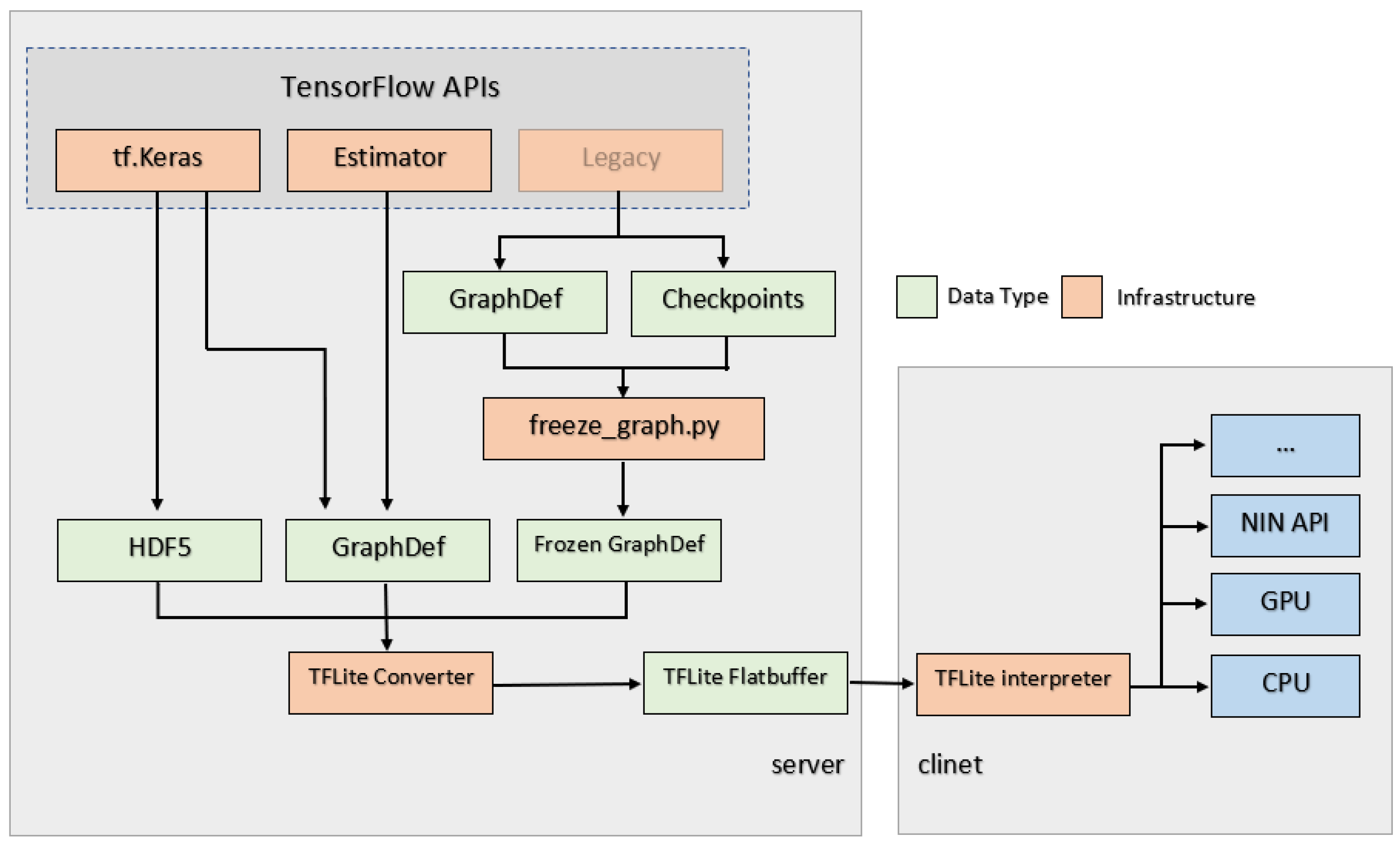
Figure 8 demonstrates the flowchart of how TensorFlow Lite works. When the model is fixed, it can be saved in a format containing both of its graph and weights so that the model can be frozen to a .pb file with its graph and weights, and only this format can be recognized in Android App (for TensorFlow Lite, it should be a .tflite file). During the process to freeze the model, all variables used in training would be converted to constants.
4.2.3. Flowchart
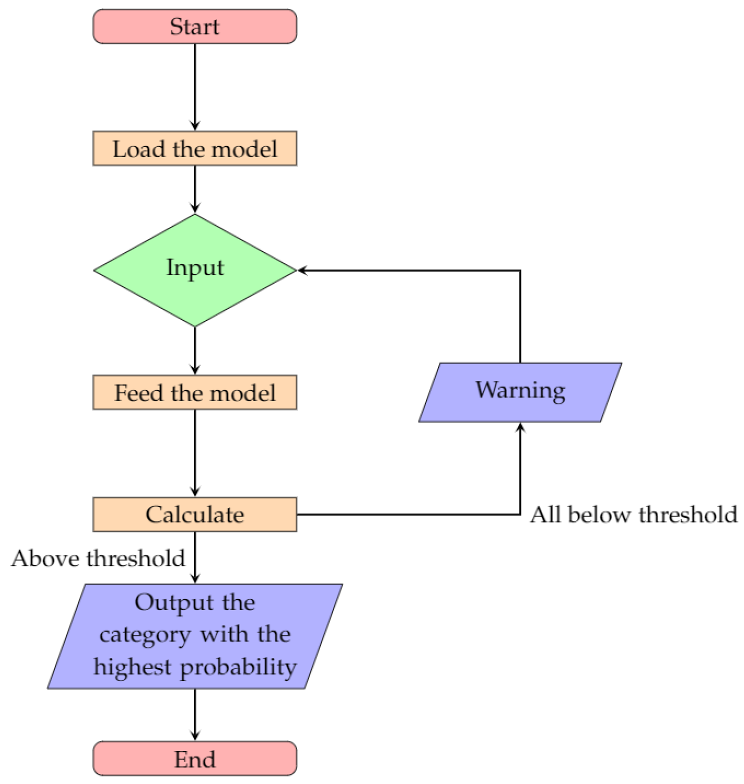
In this Android App, the model will be loaded first, including the label file. The label file contains ten butterfly category names, their main features and their indexes which were used in this App (every name is a label). Users can choose an image either by taking a picture with the camera or selecting one from the gallery. The chosen image will be fed into the model and the model can start to calculate the probability of each category. Then the system determines the category with the highest probability as the output. However, the highest probability has to be above a threshold, or the App will throw a warning "The target is not likely to be in the following butterfly categories: Danaus plexippus, Heliconius charitonius, Heliconius erato, Junonia coenia, Lycaena phlaeas, Nymphalis antiopa, Papilio cresphontes, Pieris rapae, Vanessa atalanta, and Vanessa cardui." In this paper, the threshold is 0.5 to ensure that there will not be more than one output due to the same probabilities. The flowchart of the developed application is shown in
Figure 9.
5. Experimental Results and Discussions
Usually, after models are built, they need further optimization to achieve the best accuracy. The optimization process is a time-consuming and experience-oriented task. Multiple parameters need to be configured and we tested several of them in this paper. The parameters with which we have tested included Data Augmentation, Batch Size, Batch Normalization, and Optimizer. All experiments were conducted on a device with NVIDIA GeForce GTX 1080 Ti GPU and Intel(R) Core (TM) i7-8700K CPU.
5.1. Optimization
5.1.1. Data Augmentation
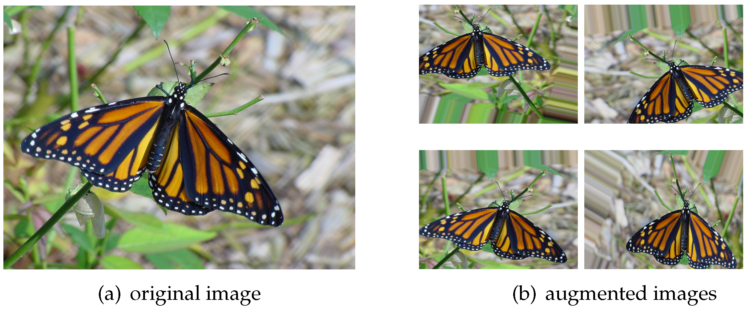
The quality and quantity of datasets are always a concern to researchers and developers as this will affect the accuracy of machine learning algorithms. The common problems are overfitting and underfitting. The easiest way to alleviate these problems is to increase the sample size in the training set as it can be beneficial to extract image features and generalize models. In machine learning, we sometimes cannot increase the amount of training data because it is costly to find labeled data. However, the dataset can be expanded by rotating, cropping, shifting, scaling, transforming the images, and so on. Although the augmented images are almost the same as the original image in human beings’ vision, they are new data structures from the perspective of a computer as the data arrays, which are used to describe the pixel information to a computer, are changed. In this way, we can generally improve the accuracy of the model, and it is also a common technique for optimizing the model, as shown in
Figure 10.
After applying the augmentation technique, there are 4160 images in total. We used 60% (2496 images) of the dataset as a training set, 20% (832 images) of the dataset as a validation set and 20% (832 images) of the dataset as a testing set. All sets are independent. In this paper, all the results shown in tables are testing accuracy.
SVM
With SVM, data augmentation has no obvious enhancement as the size of the original dataset has already challenged the models, especially that this is a ten classes classification task.
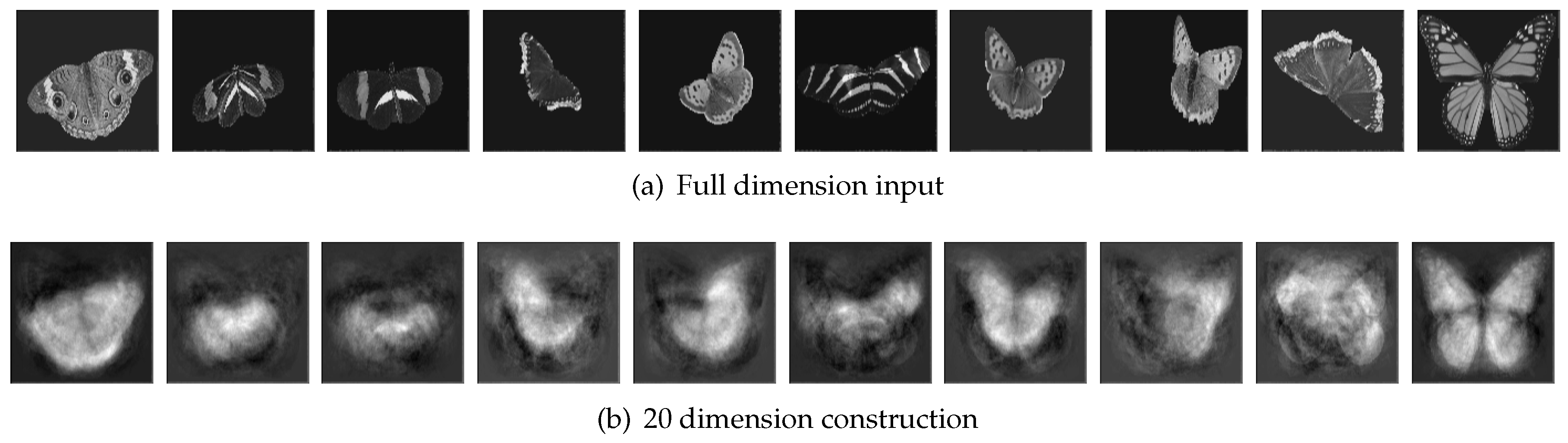
Table 1 shows the accuracy of the PCA/SVM method and it implies that the highest accuracy 52.6% occurred when the top 20 components were extracted by PCA.
Because the overall accuracy was the highest when 20 principal components were extracted, we visualized the contrast of original input images and their 20 principal components as
Figure 11. From this figure, we can understand better that PCA reduced the complex dataset into a simplified dataset with 20 components that can express the information of the dataset best.
RF
Similar to SVM, we first conducted experiments without and with data augmentation, respectively. However, RF did not show any improvements after data augmentation. Then we tried to apply PCA before RF with the original dataset. However, there are no significant enhancements either and most of the results are even not as good as without using PCA. We believe the reason PCA prior RF is not a great advantage is that RF already performs a good regularization without assuming linearity, PCA is not necessarily an advantage. Consequently, we take the result of 350 trees with data augmentation and without PCA as the best performance of RF, as shown in
Table 2.
4-Conv CNN and VGG19
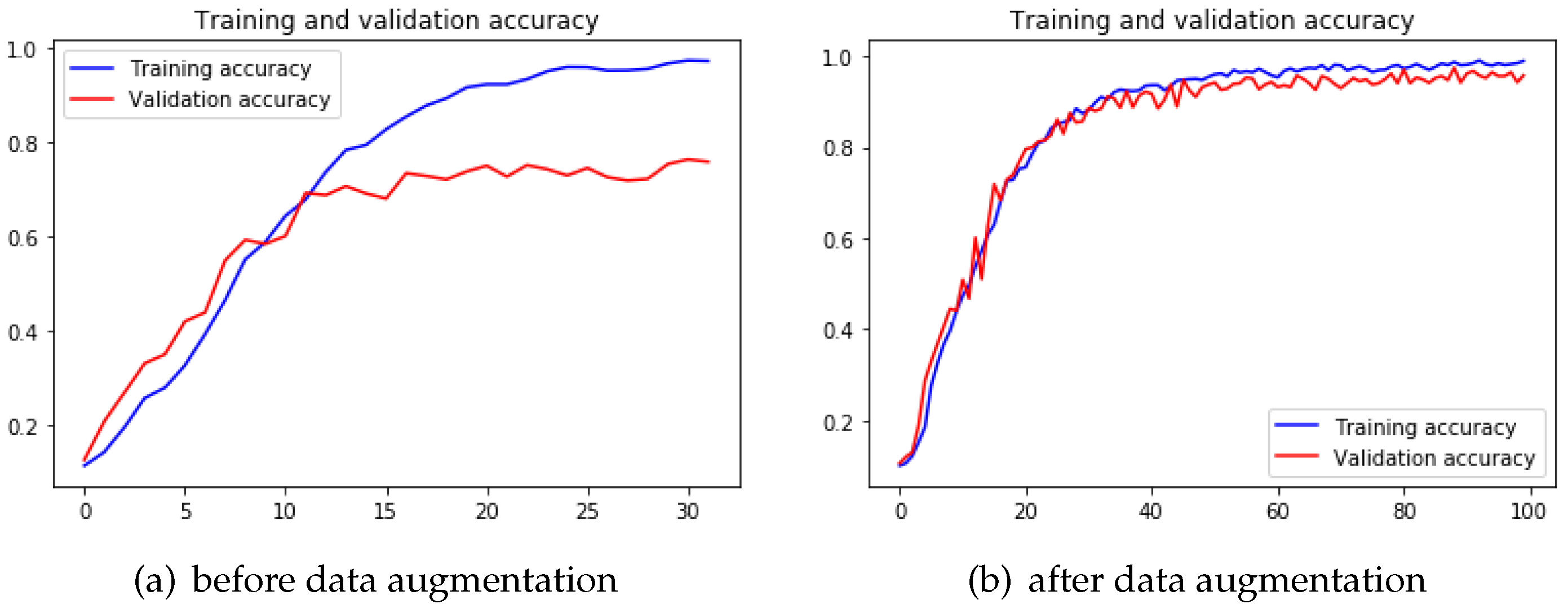
When it comes to 4-Conv CNN model, we notice typical o%verfitting after training this model. With certain epochs of training, the validation accuracy of this model started to keep stable while the training accuracy was still increasing. The validation accuracy stopped to increase after 15 epochs of training (
Figure 12a), and the testing accuracy ended up with
on 4-Conv CNN model. After applying the data augmentation technique, it is clear that the 4-Conv CNN model overcame the early overfitting problem (
Figure 12b). In transfer learning, the pre-trained VGG19 model also showed improvement after data augmentation.
Table 3 shows that performance of both the 4-Conv CNN model and VGG19 model improved so that we have determined that data augmentation indeed prevents overfitting problem to a large extent with deep learning algorithms.
5.1.2. Batch Size
When comparing the results of training with different batch sizes in
Table 4, it is noticeable that the final accuracy with 64 is higher than that with 128 in both groups.
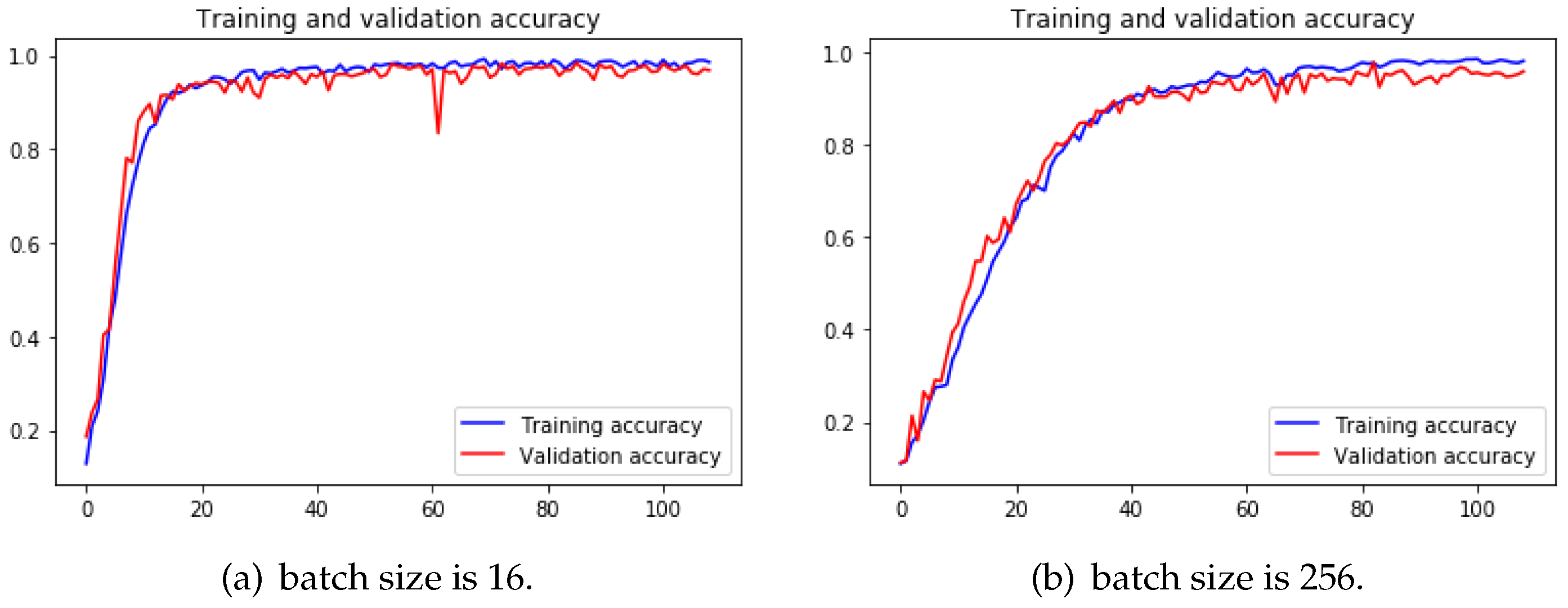
The reason why small batch sizes perform better is that small batch size brings a more stochastic factor to the learning so that the learning has more chances to leave the local minimum and keeps looking for the accurate gradient direction. Although training with large batch size needs less time to finish a training epoch, more epochs are needed to reach the same precision as the small batch size, or even could not reach the same precision. Small batch size causes the loss function to fluctuate severely if the network is deeper and wider. To make the difference more obvious, we trained 4-Conv CNN with a batch size of 16 and 256, and we can observe from
Figure 13 that when batch size is 256, it took more epochs to arrive at a similar accuracy than the other one.
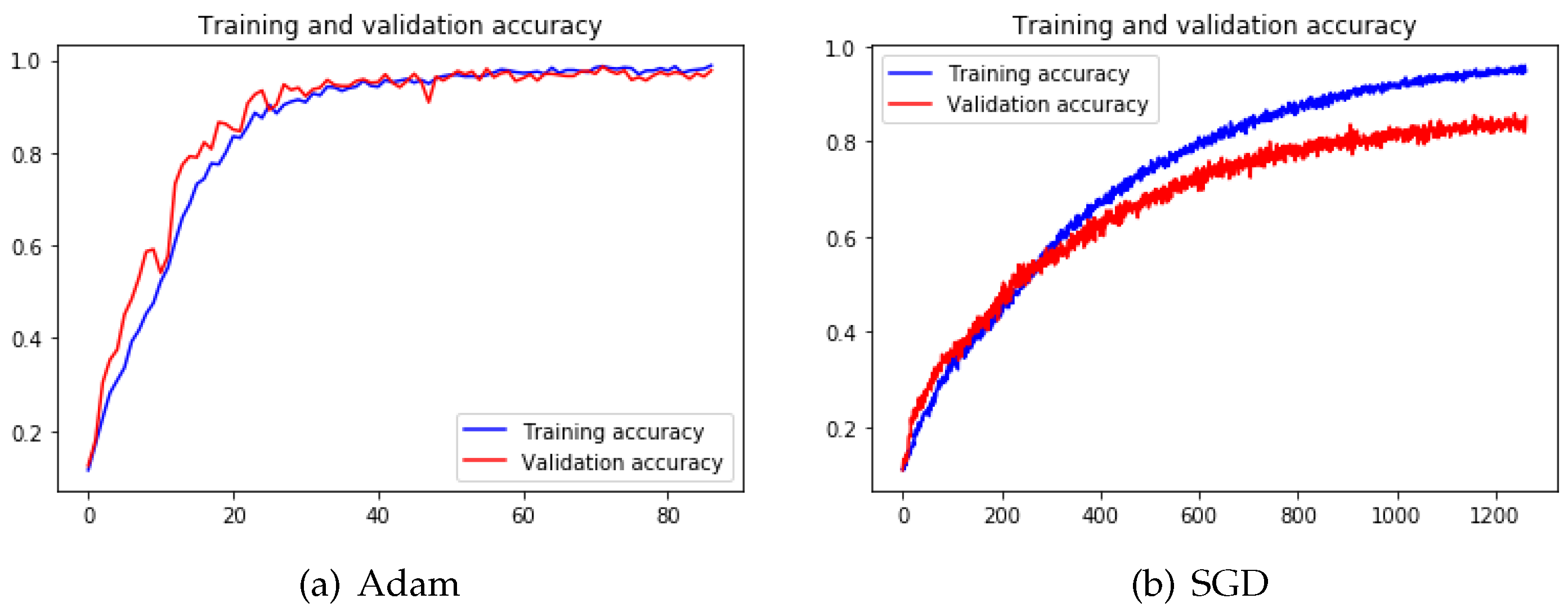
5.1.3. Optimizer
With conducting experiments on 4-Conv CNN and pre-trained VGG19 models, we can notice that the Stochastic Gradient Descent (SGD) [
35] needs much more epochs and time to converge and the final accuracy is lower than the other two methods from
Table 5 and
Table 6.
Figure 14 illustrates that the fluctuations during training with the SGD process are way more dramatic than training with Adam [
36]. The reason is that the mechanism kept adjusting itself to search for the correct gradient direction. However, the training has not been converged even after 1200 epochs.
Because of the limited computing resources, we did not test SGD on other models and we adopted Adam + SGD as our default optimization method. This hybrid of Adam + SGD method means that we used Adam as the optimizer to train the model first because of its self-adaptive ability and fast speed, but we applied SGD with a relatively low learning rate (0.00001) to train the model at the later training phase to avoid missing the optimal solution.
5.1.4. Batch Normalization (BN)
VGG model does not have BN layers because BN did not exist before it, so we did not add BN to this pre-trained model. Also, it would change the pre-trained weights by subtracting the mean and dividing by the standard deviation for the activation layers [
37]. Thus, we did experiments only on the 4-Conv CNN model. Although the testing accuracy after adding BN layers is slightly higher than without BN (
Table 7), it took fewer epochs to converge than training without BN. It is because the BN layer enables faster training by using much higher learning rates and alleviates the problem of poor initialization.
5.2. Comparison between Final Results of Different Methodologies
After several attempts to optimize all models, we summarized the best performance of each model. From
Table 8, we learn that deep learning outperforms traditional machine learning. Although the accuracy of the 4-Conv CNN model and the re-trained VGG19 model are very close, according to Occam’s Razor [
38], we chose 4-Conv CNN model to embed in Android App as its architecture is simpler than VGG19. The average predicting time of the model is 3653 ms.
Because the structures of SVM and RF are shallow and simple, the only way to enhance the performance is to integrate other algorithms into the existing models. This is why the main task in traditional machine learning area is to search for suitable algorithms, while the chief problem in deep learning is to adjust suitable parameters as the layers in deep learning are relatively easy to understand, but the process to combine different layers and to adjust parameters is complicated and time-consuming. When it comes to large datasets and complex scenarios, deep learning methods are dominant.
5.3. Android Application
5.3.1. Structure
In this Android App, we have three classes which are MainActivity, TensorFlowImageClassifier, and Classifier. The deep learning model and label file were uploaded to the assets file. An image can be passed to the model loaded in TensorFlowImageClassifier, where the label file is also loaded. After the model successfully accepts and predicts the data, the index of the label and the confidence (probability) of the result released from the output interface of the model are passed to the class Classifier. Then the predicted label and the description of the image will be returned to the TextView defined in MainActivity, and the confidence of the predicted label will be shown in the TextView at the same time.
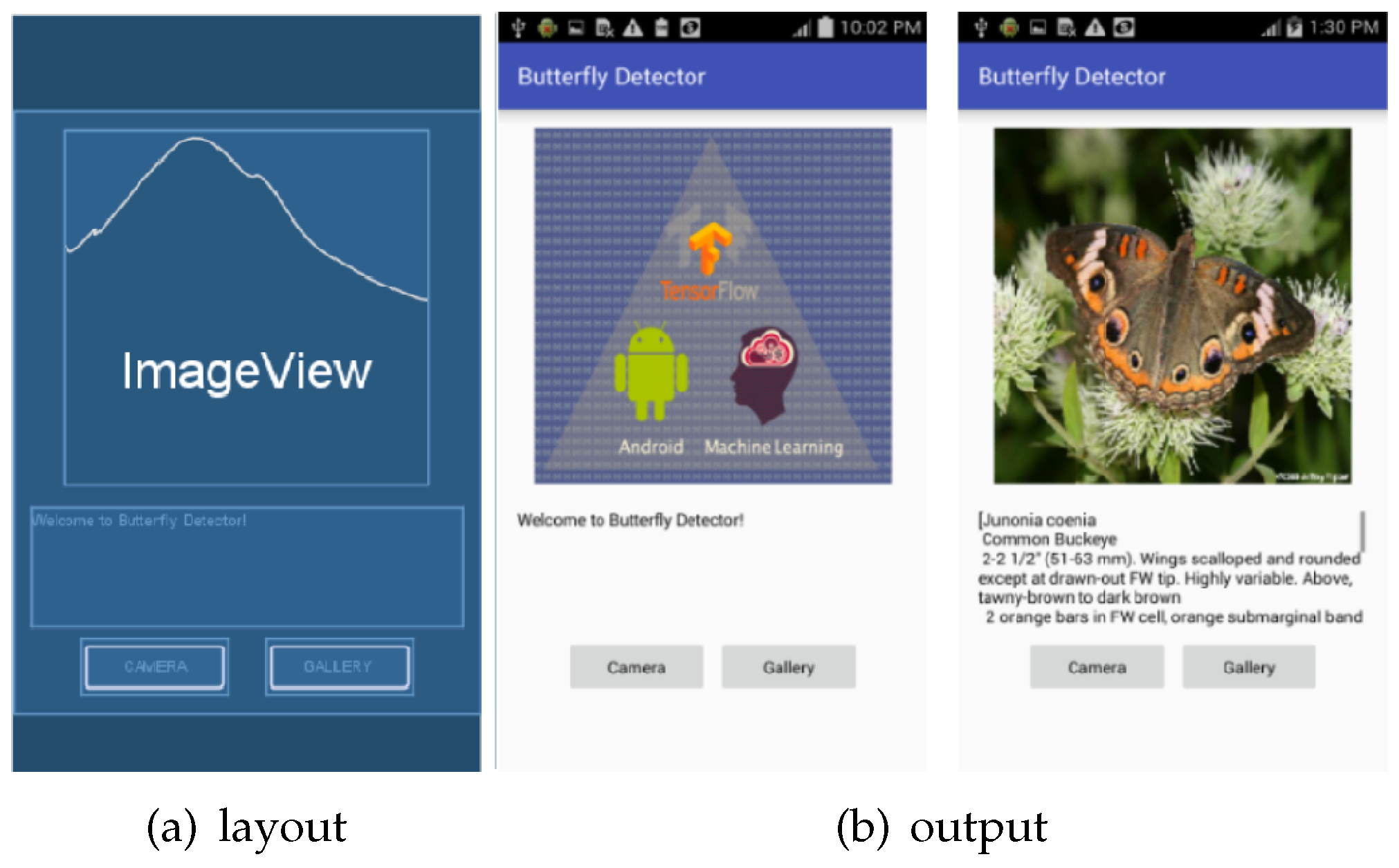
5.3.2. Layout and Output
The layout includes an ImageView, a TextView and two buttons, shown in
Figure 15. An image can either be captured by the camera or selected from the gallery and it will be shown on the ImageView. Images from both the camera and gallery will be processed and sent to the classifier in the same way. Then the returned label and description are on the TextView.
5.3.3. Performance
Because the images can be input from either a smart phone’s camera or gallery, we tested on 20 images taken by the camera of the smartphone, such as
Figure 16, and 20 online open-source images in the smart phone’s gallery. In both groups, half of the images belong to the ten classes in the model whereas the other half are excluded from the said 10 classes. All images of butterfly specimens and alive butterflies in this experiment were taken in a Butterfly Conservatory (Cambridge, Canada).
It cost 363 ms for the App to load the model and the average time to predict an image’s category (from inputting the image to outputting the result) is 3278 ms. The confusion matrices as
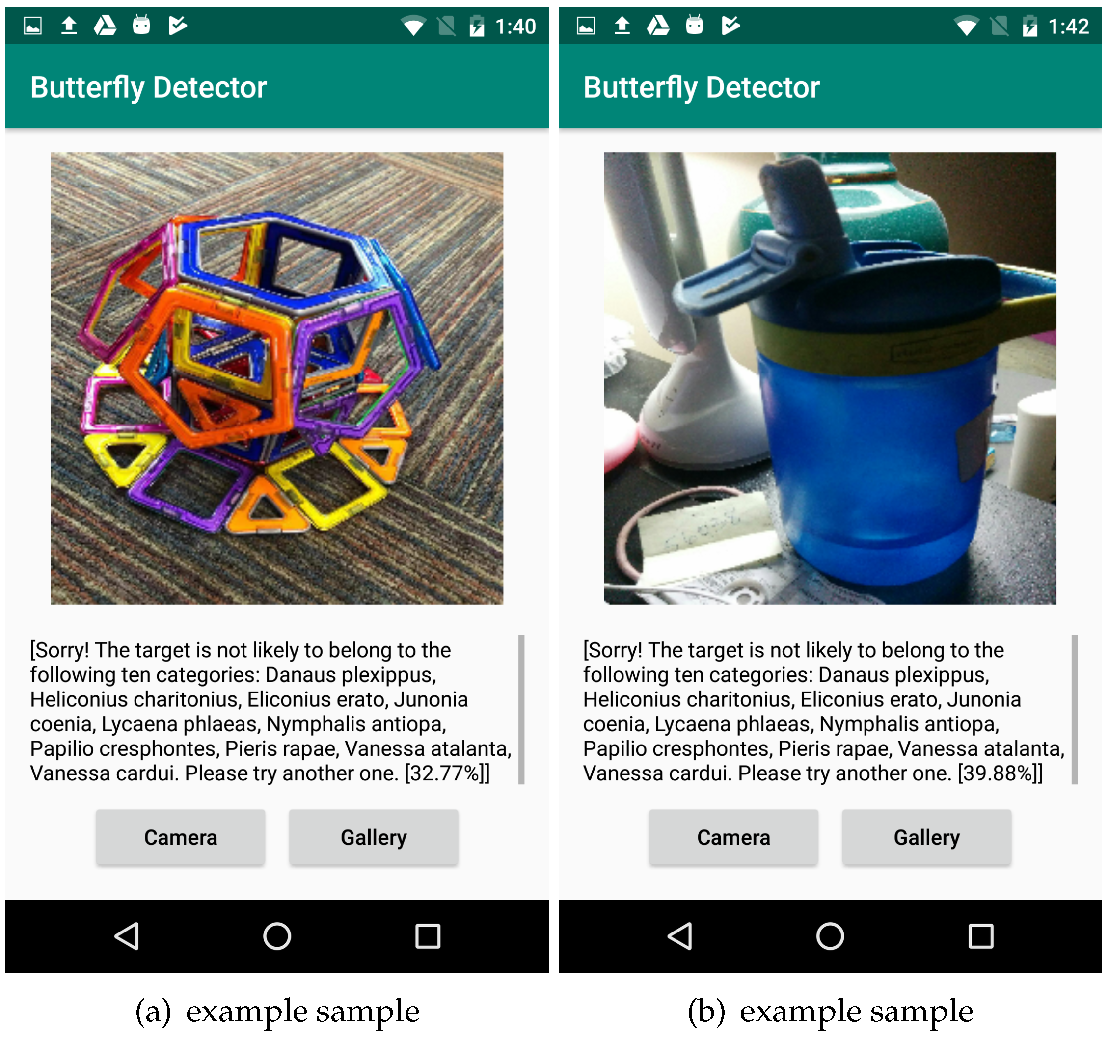
Table 9 show the performance of the App in real scenarios. The confusion matrices show that in both groups, some input classes which are not in the training dataset can be easily predicted as one of the classes in the training dataset. The reason for this is that the patterns of different butterfly categories can so resemble that the model will predict it as the most similar one in the training dataset. However, when the system predicted images of non-butterfly objects, such as a water bottle and a toy in
Figure 17, the output can throw a warning that this target is not likely to be a butterfly in the ten categories because the highest probability is below 0.5 (the value at the end of the output is the highest probability.). The 4 and 2 true negatives (TN) in the two confusion matrices are the correct prediction of non-butterfly objects.
Table 10 shows the evaluation of the App’s prediction performance. There is no significant difference between the prediction results of images from the camera and gallery.
Because there are only ten categories in the training dataset, when predicting butterflies other than these ten categories, there is a high possibility that they will be predicted as one of the ten categories. To solve this problem, we need to collect a larger training dataset including categories other than the ten categories. Only in this way, the system could predict more butterfly categories precisely.
5.4. Summary
Users can use this Android application to distinguish different kinds of butterflies with ease. Compared to save models on servers, this application’s superiority is that it does not require communication between server-side and client-side, which makes this application can be used in an environment without network connectivity. This advantage is crucial when butterfly researchers are working in a wild area lacking network. From this perspective, we are convinced that implementing deep learning algorithms in a limited resources platform, e.g., mobile, is essential.
The model we stored on the device is 82M, and the final application is 322M. If a neural network is more complex than the one we adopted in this project, the model itself would be hundreds of megabytes, which is usually unacceptable for mobile device users. There are optimized_for_inference and quantized_graph methods in TensorFlow that can delete unnecessary nodes and compress the model to reduce the size of the model, but the trade-off is that the accuracy of the model would decrease to some extent. We have optimized our model with the tools and the output file is only a quarter of the original one. However, the model stopped working. Therefore, we still used the original model to build the App, but we will search for the reason for failure in future work.
To improve the application, we need to collect more categories of butterfly images. If we could collect more butterfly categories to train the model, then it is reasonable to expect the app’s performance to be significantly improved.
6. Conclusions
This paper proposed an Android application for detecting butterfly categories. We have presented a description of building and optimizing several models to choose an ideal one that can be deployed to an Android mobile device to classify butterfly categories. These structures include the traditional machine learning models (SVM and RF), deep learning architecture (4-Conv CNN) and transfer learning pre-trained model (VGG19). During the process of training all these models, we also adjusted the parameters to find the optimal one. The results show that different models are sensitive to the choice of parameters. For example, with SVM, when the amount of data reached a certain amount, the testing accuracy would not improve anymore because they cannot handle complex scenarios. However, the data augmentation operation has a significant meaning to 4-Conv CNN, while the transfer learning method is not sensitive to the size of this butterfly dataset either because the domain of this dataset is very similar to their original domain. Therefore, selecting tuning parameters requires patience and experience as the choice of tuning parameters depends on the architectures of the model and the objective of the project.
At last, we converted the optimal model to a format that can be executed in an Android application with TensorFlow Lite. The result shows that it is feasible to use deep learning models on mobile devices while preserving the accuracy of the model. However, we still need to figure out how to further optimize the model so that the size of the model file could be compressed, and this would prompt users to download the application. We believe this butterfly detection Android application will bring convenience to butterfly researchers and the industry and that it is essential that more deep learning algorithms be integrated into mobile applications.


