Abstract
The structure of fibrous assemblies is highly complex, being both random and regular at the same time, which leads to the complexity of its mechanical behaviour. Using algorithms such as machine learning to process complex mechanical property data requires consideration and understanding of its information principles. There are many different methods and instruments for measuring flexible material mechanics, and many different mechanics models exist. There is a need for an evaluation method to determine how close the results they obtain are to the real material mechanical behaviours. This paper considers and investigates measurements, data, models and simulations of fabric’s low-stress mechanics from an information perspective. The simplification of measurements and models will lead to a loss of information and, ultimately, a loss of authenticity in the results. Kolmogorov complexity is used as a tool to analyse and evaluate the algorithmic information content of multivariate nonlinear relationships of fabric stress and strain. The loss of algorithmic information content resulting from simplified approaches to various material measurements, models and simulations is also evaluated. For example, ignoring the friction hysteresis component in the material mechanical data can cause the model and simulation to lose more than 50% of the algorithm information, whilst the average loss of information using uniaxial measurement data can be as high as 75%. The results of this evaluation can be used to determine the authenticity of measurements and models and to identify the direction for new measurement instrument development and material mechanics modelling. It has been shown that a vast number of models, which use unary relationships to describe fabric behaviour and ignore the presence of frictional hysteresis, are inaccurate because they hold less than 12% of real fabric mechanics data. The paper also explores the possibility of compressing the measurement data of fabric mechanical properties.
1. Introduction
1.1. General Context
The advent of the digital age has put forward increasingly stringent requirements on the authenticity of fabric models and virtual simulations. A model must be able to characterize its static and dynamic behaviours in a way that is close enough to the mechanical behaviours of real fabric. When people interact with fabrics in a virtual space, they can get close to the same visual and mechanical experience as interacting with fabrics with the same mechanical properties in the real world and experience the real aesthetics of fabrics and clothing. Applications such as CAD, product development, internet shopping, virtual environments, film, TV and advertising, medical simulations and computer games can make technical and business decisions through virtual simulation across time and space environments. In the process of intelligent customized design, manufacturing, and use of clothing for certain special applications such as medical, competition sports, and military, there are strict requirements for the authenticity of fabric mechanical models. With the development of wearable information technology, more and more flexible sensors and energy-autonomous devices use fabrics as their base materials. These sensors and devices often require rigorous software correction for nonlinearities caused by the substrate material to ensure their overall performance. Fabric mechanics, as the basis for domain-end digitalization, must be developed to guarantee and meet these new needs.
The need to realistically characterise and simulate the mechanical behaviour of fabrics is urgent and necessary. As early as 1998, Stylios [1] and Hearle [2] argued that the textile and apparel industry faced challenges in transitioning from empirical craftsmanship to engineering. It is imperative to develop software that is acceptable and usable for the industry. Software must be able to realistically characterise the behaviour of complex fibre components based on calculations of simple relationships. With the need to develop powerful digital virtual tools such as digital twins, the challenges facing the industry are far more demanding and complex than just a shift from empirical to engineering practises alone [3]. In the textile and apparel industry, the integration of digital information technology with fabric modelling and simulation technology will involve the full life cycle of industry products such as demand definition, fabric design, fabric manufacturing, clothing silhouette and art design, clothing process design, clothing design verification, clothing manufacturing, packaging design, clothing sales, product use and recycling, market prediction and feedback. Virtual digital twins of fabrics and clothing will interact with real-world physical presences. Fashion is a highly personalised product usually following a trend. It is inevitable that users are deeply involved in the customisation and design of clothing through virtual means. There is an urgent need to solve the problem of realistic characterisation of the mechanical behaviour of fabrics in a virtual environment.
Using the output of a fabric mechanics model to truly represent the mechanical behaviour of a fabric is inextricably linked to both the input information obtained by the model and the model’s ability to process this information. The important aspect is that the model’s heuristic input (virtual) information is a complete subset selected from an infinite set of possible input information. The model must be designed so that its rules and knowledge can accurately handle each possible choice and generate corresponding output information. Only in this way can the model be used to explore various possible subsets of input information to eliminate the uncertainty in its corresponding predicted output and optimize the design of fabrics or clothing in applications. Here, the completeness of the input information means that the virtual information subset must meet the model’s dimensional requirements for input information. During model design, the specific content of heuristic input information is unknown, but its dimensions must be determined.
A fabric mechanics model can be viewed as a set of multivariate nonlinear function mappings. At the heart of the mapping relationship are proven rules and knowledge of fabric mechanics. If overall authenticity in the model’s output information is expected, then two prerequisites must be met. The first prerequisite is that the model must obtain complete material mechanical property information, geometric information, force constraints and condition information of the fabric that can truly represent its mechanical behaviour. The second prerequisite is that the model must have rules and knowledge that can correctly and effectively match and process the input information. A complete set of input information must include all information dimensions that have a significant impact on the mechanical behaviours of the fabric. The model itself does not create information; it can only generate output information from input information according to the rules and knowledge it has. If the completeness of the dimensions of the input information and the rules and knowledge of the matching model cannot meet the requirements, the output information of the model will inevitably not have overall authenticity.
1.2. Considering Fabric Mechanics
The acceptance of deviations in mechanical behaviour simulation caused by the inability to provide and process mechanical property information and the oversimplification of the complexity of fabric mechanics depends on the application. (Ngo and Boivin, 2004) and (Stylios, 2008) pointed out that many methods for simulating clothing, despite having interesting visual effects, cannot be used in the textile and clothing industry due to a lack of realism [4,5]. Other researchers observed hysteresis up to 50% of the mean force, and they suggested that neglecting internal friction could lead to deformation errors of up to ±25% for a given load [6]. Additionally, they observed that internal friction plays a central role in the formation and dynamics of fabric wrinkles and folds. (Volino et al., 2009) believe that the highly nonlinear and anisotropic mechanical properties of cloth pose challenges to accurate mechanical behaviour simulation [7]. (Wang et al., 2011) state that most fabric simulation techniques ignore the nonlinearity and anisotropy of fabrics [8]. Although these simplified models can produce reasonable results, they cannot accurately represent the nature and core behaviour of real fabric mechanical properties or distinguish different fabrics. In fact, the so-called “hyper elasticity” and oscillation stability that appear in many cloth simulation algorithms are caused by the negligence of nonlinear mechanical properties and internal friction information. (Miguel et al., 2013) reported how they used Dhal’s frictional model to simulate the nonlinear bending behaviour of two fabrics, recognising branching complexities and not considering shear [6]. (Wang et al., 2019) reported that cloth is a highly mouldable material and undergoes a wide range of deformations [9]. They recognised that problems with modelling and simulating various mechanical properties could directly affect the accuracy of cloth simulation. They have also asserted that despite many years of in-depth research, various outstanding problems in cloth simulation persist. In a recent FE study, researchers confirmed that “the dissipative performances of woven fabric under tension resulted from the synergistic effect of the material’s viscoelasticity and surface friction among yarns of fabrics, and also the higher friction coefficient of the yarns contributes to a better stability in dimension and morphology of the fabric [10]”.
How to identify and determine the impact of fabric mechanical information dimensions on fabric behaviour is challenging for model design, fabric measurement instrumentation and usage selection. The high degree of complexity of a fabric’s structure leads to the complexity of its mechanical behaviours. Within the linear elastic range of the material, the stress–strain relationship for a homogeneous and isotropic linear elastic material can be fully characterized using its physical parameters and linear constitutive equations. These physical parameters usually include Young’s modulus, Poisson’s ratio, shear elastic modulus and unit volume mass [11,12]. Through simple tension and shear measurements, the mechanical parameters of the Hooke body can be easily obtained. If a set of material geometry, dimensions and force are given, the calculation can use a rigorously verified elastic mechanics model to predict the stress–strain relationship of linear elastic fabric and the behaviours of the material in the virtual space–time environment. This is the basic premise for the widely accepted and applied Hooke body mechanics simulation. But the fabric is a specially assembled fibre structure rather than a Hooke body. To date, the understanding of fabric structures and their mechanical behaviours remains limited. It is well known, however, that the deformation of a given fabric structure includes the following characteristics: Nonlinearity, Hysteresis, Anisotropy, Large deformation, and Time dependence, with Frictional Hysteresis being very important but highly complex at the same time. Consequently, this paper aims to provide answers about the complexity of the frictional hysteresis component of fabric mechanics and whether it can be simplified or ignored. Recognising that most fabric mechanical data is produced through uniaxial measurements of how significant the information loss is, and finally, how we can compromise between model accuracy and computational complexity.
2. The Challenges of Defining Fabric Mechanical Behaviour
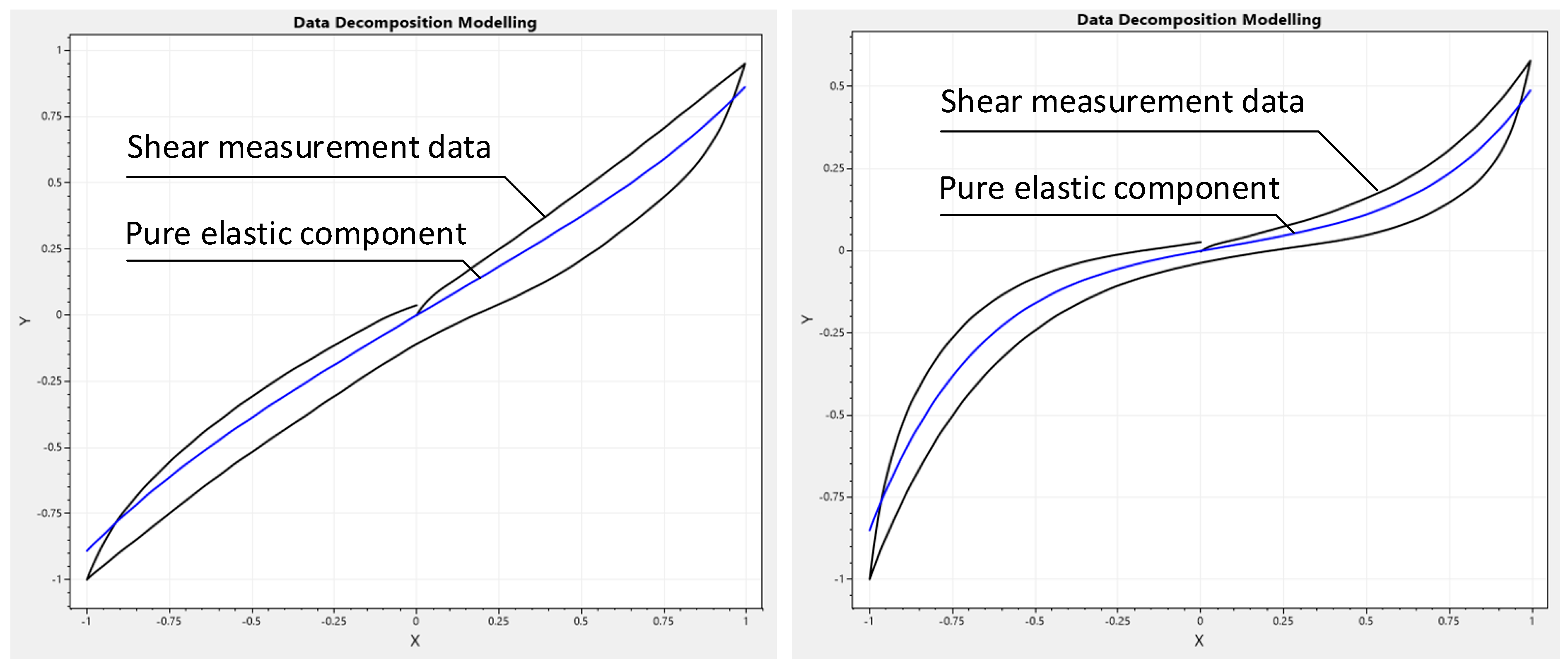
These characteristics are intertwined and complicate the construction of reliable models to describe their mechanical behaviours. The uncertainty in the mechanical behaviours of fabric structures far exceeds that of Hooke bodies. It also shows that using simulation models to predict the uncertainty caused by poorly determined fabric mechanical characteristics, geometric dimensions and forces requires models with far more rules and knowledge. Due to the use of different fibre materials, textile processing techniques and weaving structures, the mechanical complexity of different fabrics also varies greatly. This variability causes the method of comparing the mechanical behaviours of physical fabric samples with model predictions for determining the authenticity of the model to lose significance. For example, in the author’s fabric measurement database, measurement data No. 147 and No. 20 indicate that the shear characteristics of the two fabrics have different nonlinear complexities. The data in Figure 1 have been normalised. The purely elastic components contained in the measured data are decomposed from the data. On the left is the measurement data of Fabric No. 147. It contains a purely elastic component that approximates a straight line. The properties of this fabric sample can be approximated using a linear elastic model. On the right side is the measurement data of Fabric No. 20. Its purely elastic component has a higher nonlinear complexity than the purely elastic component of the measurement data of Fabric No. 147. Satisfactory results will be obtained using the shear behaviour of fabric sample No. 147 compared with the predictions of the linear elastic model. But using the same model to predict the shear behaviour of fabric No. 20 will result in unacceptable errors.
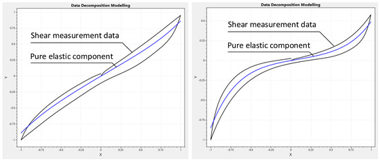
Figure 1.
Measured data on the shear properties of two fabrics of different complexity and the pure elastic component they each contain.
Since biaxial measurement of fabric in-plane deformation faces many challenges, the characteristic parameters of fabric mechanics often come from some simple traditional measurement methods or uniaxial instrument measurements. Can the data obtained by these simplified measurement methods support a model of the true mechanical behaviour of the fabric? Or how much information loss do they result in? We need to make the necessary assessments of these data.
Modelling and developing measuring instruments for complex fabric mechanical behaviour require a theoretical tool that can be used in advance to evaluate and quantify the impact of different fabric measurement and modelling methods on the effectiveness of the obtained mechanical characteristics. Hence, with a wide variety of simplified fabric property models and simplified measurement methods, the loss of information due to simplification can be evaluated. Assessments can help us identify existing gaps and identify directions for further research. Tools can also be used to specifically quantify the information needed in fabric measurement data, and management of data obtained through measurements using compression can be achieved, which is also relevant in our digital age.
However, in the existing literature on textile mechanics, models, and simulations, we have not yet found a simple and powerful information assessment tool. To bridge this gap, we introduce Kolmogorov complexity (algorithmic information theory) into the study of fabric mechanics. In Section 3 we will review the most basic concepts of information theory and Kolmogorov complexity, and we will introduce the stress–strain and friction–hysteresis relationships of fabric mechanics. Polynomials are used to approximate the multivariate nonlinear mechanical relationships. In Section 4, Kolmogorov complexity is applied to analyse and compare them to determine the information relationships of fabric mechanics and evaluate the algorithmic information loss of simplified relationships. To facilitate understanding of the complexity of Kolmogorov, we use enumeration to describe examples and then discuss these contents in a simple induction way. In Section 5, we bring together the important information analysis results of fabric mechanics and consider and discuss the impact of these results on the future development of fabric instrumentation, fabric modelling and simulation.
3. Shannon Information Theory and Kolmogorov Complexity
Information is a key concept across multiple disciplines in natural sciences, humanities and in people’s daily lives. Everything we know about the world is based on the information we receive or collect, and in principle, every science involves information. However, researchers such as (Barbieri, 2016) and (Rocchi, 2012) show that there is still disagreement on the appropriate definition of information [13,14]. Wiener believed that information is not matter or energy; information is information. It is the name of the content that people exchange with the objective world in the process of adapting to it. That is to say; Wiener believed that in the space–time environment, information has the same level as matter and energy [15].
The philosophical meaning of information is a complex issue [16], a polymorphic phenomenon, and a polysemantic concept that can be associated with multiple interpretations [17]. In the general field of information theory, it is likely that at least some of the many different semantics assigned to information by different authors will prove useful enough in some applications. They deserve further study and recognition. It is difficult to expect that the numerous possible applications in this area can be satisfactorily explained using a single concept of information [18].
In the fields of information processing and communications, due to the need to design effective data encoding and transmission methods, two basic questions must be answered: the minimum limit level that data compression can achieve and the ultimate rate of data transmission. Hence, a quantitative concept of information needs to be established. (Nyquist, 1924) expresses the amount of ‘intelligence’ that a telegraph system can convey at a specific linear speed using a logarithmic function of the number of loop current values [19]. (Fisher, 1925) proposed a method of measuring the information content of observable random variables from a statistical perspective [20]. (Hartley, 1928) constructed a function to quantify the amount of information obtained when an element is selected from a uniformly distributed finite set [21]. Its information content is the logarithm of the cardinality of the set. (Shannon, 1948) created the mathematical theory of communication (MTC), known as Shannon’s information theory [22]. Shannon defined information as a description of uncertainty about the state of things or the way they exist. Information is the content of any communication. The direct purpose of eliminating the sink’s uncertainty about the source message is achieved through communication. The amount of information is equal to how much uncertainty is eliminated. Shannon introduced the concept of entropy to measure this information uncertainty.
3.1. Shannon’s Information Entropy
Definition: Let the sample space of the discrete random variable X be , where the probability of an event occurring is denoted as , , and the self-information of the event is given using the following equation:
The unit of self-information in Equation (11) is a bit.
Theorem: The entropy of a discrete random variable X is the expected value of its self-information:
Shannon’s information theory [22] has achieved great success in information transmission, encoding, storage and data compression. It does not involve the semantics of the information itself, so it is also called syntactic information theory.
3.2. Algorithm and Kolmogorov Complexity
The algorithm is based on the understanding and decomposition of the logic of a problem and uses a certain effective finite series of simple mechanical operations to solve the steps or sequence of the problem. Algorithms infuse problem-solving knowledge and intelligence into computational machines. The time and space complexities of the algorithm are used to analyse and judge the advantages and disadvantages of the algorithm. Algorithms are the foundation of computer science and the core of continued research in this field.
Kolmogorov complexity (algorithmic information theory) provides a new perspective on the concept of information. It uses the binary encoding length of the shortest description program of an information object to measure its information content. Algorithmic information theory was proposed and developed by Kolmogorov [23,24,25], Solomonoff [26,27,28] and Chaitin [29]. It is based on the Turing machine computational model [30] and the optimization of the program algorithm description dimension according to the parsimony rules of Occam’s razor. Its main results clarify the concepts of randomness and probability. In a rather different context, algorithmic information theory reproduces the results of Shannon’s information theory [31]. The following definitions and theorems refer to the above-mentioned references on Kolmogorov complexity and the work of Cover and Thomas [32].
Definition: Let us s be a binary string of limited length, and Tu be a general computer (Turing machine). When a program p is given, is the binary string length of p. Let be the output of Tu with respect to program p. Then the Kolmogorov complexity of the binary string s is as follows:
That is, the Kolmogorov complexity is the minimum binary string length of all programs that can output s and stop (satisfying computability). If the binary string length of s is known, then
If p does not exist, then
In the above definition, program p is used to describe s. That is, the Turing machine Tu uses its input program p to generate the described object s.
Invariance theorem: Suppose K1 and K2 are the complexity functions of the description languages L1 and L2 that satisfy Turing completeness, then there is a constant C. The choices for the description languages L1 and L2 are
Theorem: For a binary output string s, is its length, and there exists a constant C such that
Theorem: For any , there is a complexity of string s:
Theorem: K is not a computable function. That is, there is no program that can take the string s as input and then obtain its K(s).
Kolmogorov’s chain rule of complexity is given using
That is, the shortest program describing X and Y differs by one logarithmic term from the sum of the shortest program describing X and the shortest program describing Y, respectively.
3.3. The Relationship between Kolmogorov Complexity and Information Entropy
Theorem: If X1, X2,… are independent uniform integer random variables, and the entropy is H, there exists a constant C for all n, then
3.4. Mathematical Abstraction of Low-Stress Mechanical Properties of Fabrics
To support the analysis of the algorithmic information of stress–strain fabric relations using Kolmogorov complexity, the contents of this section bring together a summary of fabric stress–strain and their friction hysteresis relations [33,34].
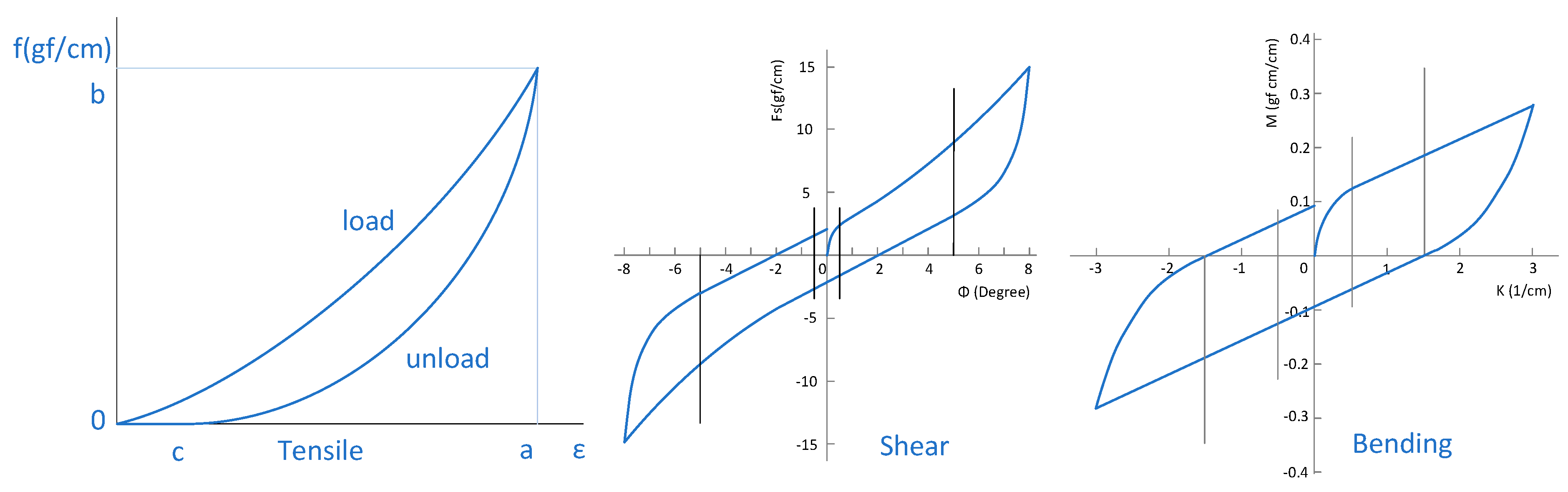
The mechanical properties of woven fabrics are usually divided into stress–strain relationships of in-plane deformation and bending deformation. In-plane deformation includes the stress–strain relationship of longitudinal/latitudinal tensile deformation and shear deformation. In these stress–strain relationships, pure elastic components and friction hysteresis components always coexist in the form of common action points and common action lines. In the uniaxial tension, shear and bending measurement fabric data, as shown in Figure 2, due to the existence of friction hysteresis, the loading curve and the unloading curve are always non-coincident.

Figure 2.
Schematic diagram of uniaxial tensile, shear and bending stress–strain relationships of woven fabrics.
3.4.1. Stress–Strain Relationship of Fabrics
Since the magnitude of the stresses produced by bending deformations is small compared to the stresses produced by in-plane deformations, its effect on the stress of in-plane deformation can be neglected. The stress–strain relationship of fabric in-plane deformation can be abstracted, as shown in Equation (11) [35,36].
Among them, and respectively represent the pure elastic component and friction hysteresis component of fabric mechanical properties.
The bending characteristics of the fabric can be reasonably inferred as the mapping relationship between the bending force couple M and its bending curvature K, and the offset angle θ between the bending direction and the warp direction, , and . The relationship between M, K and θ has been proven in many studies [37,38]. Since in-plane shearing causes changes in fabric fibre distribution and fabric density, shearing will also inevitably lead to changes in the orthogonal relationship between warp and weft yarns. It can be reasonably speculated that shear is regarded as one independent variable in the multivariate relationship of bending properties. When a fabric is stretched, the crimped state of the fibres is changed. Since the yarns in the fabric usually have a twist, the fibres within the yarns are held tightly and change the bending section modulus of the yarns. It is also reasonable to speculate that the stretch of warp and weft yarns are used as two independent variables in the bending characteristics of the fabric. Due to the high complexity of fabric structure, there is currently no good measurement solution for the correlation between in-plane deformation and bending characteristics. So, the details of these relationships remain to be studied. To sum up, the five independent variables for the nonlinear stress–strain relationship of fabric bending can be expressed as follows:
When fabrics are subjected to repeated loads, there are problems such as accumulation of plastic deformation and hardening of fibre materials [36]. The loop formed through the hysteresis curve of its mechanical properties will also gradually change from wide to narrow and undergo spatial migration. The addition of these fabric’s mechanical behaviours will inevitably further increase the complexity of the fabric mechanics’ model.
3.4.2. Friction Hysteresis Component
Extensive research has shown that the relationship between friction and normal pressure of polymer fibres obeys a power law [39]:
where Ff represents the friction force, N represents the normal force, and a and n are regression constants obtained through data fitting, n < 1, which is approximately 2/3.
Macroscale combined deformations such as stretching, shearing, and bending of fabrics lead to complex deformations of fibres and yarns at the microscale and mesoscale [40]. With the occurrence of macro-scale combined deformation, the distribution of friction points between fibres and the normal force between fibres at friction points is constantly changing. For example, because the yarn has a twist, when a fabric is stretched, friction and self-locking occur between the fibres in the yarn, and the friction force increases with the increase in the stretching force. This allows the yarn to transmit tensile force over any length scale. The macroscopic equivalent friction force of the fabric forms a nonlinear multivariate relationship similar to that of the pure elastic component. The equivalent friction force for in-plane deformation can be expressed as follows:
Among them, i = 1, 2, 3 represent warp/weft stretching and shearing, respectively.
Similarly, for bending deformation, the following equation can be used:
To describe the hysteresis due to friction within the fabric, an extended version of Dahl’s pre-slip Model [41] was introduced:
It is worth noting that in Equation (16), fci is not a constant but a multivariate nonlinear relationship, dsi, is the path integral of the corresponding deformation.
When it is necessary to express the combination of the Coulomb friction model and the static friction model, the extended second-order Bliman and Sorine Friction Model [42,43,44,45] can be introduced.
3.4.3. Function Approximation
Polynomial space is a dense subset of the continuous function space. A series of polynomials of countable dimensions can be used to approximate continuous functions.
Let’s consider Weierstrass’s first theorem of function approximation [46]: Any continuous function f defined in the bounded closed interval [a, b] can always be approximated using polynomial Pn and the error between the two is
According to the Weierstrass function approximation theorem, nonlinear functions can be expanded into infinite-dimensional polynomial functions. The nonlinear problem of higher-order functions is transformed into the dimensionality problem of linear space. In calculations, it is often only necessary to use a few terms of a polynomial function to convey information on most fabric mechanical properties with acceptable errors.
The purely elastic components S1, S2 and S3 of the in-plane deformation (Equation (11)) and the equivalent friction forces fc1, fc2 and fc3 (Equation (14)) can be approximated using a ternary polynomial. The pure elastic component S4 (Equation (12)) of bending deformation and the equivalent friction force fc4 (Equation (15)) can be approximated using a five-variable polynomial.
The pure elastic component and the equivalent friction force of the friction hysteresis component of any fabric have different degrees of nonlinearity. This means that the degree requirements of the polynomials used to describe them also differ. The higher the degree of nonlinearity, the higher the degree of the polynomial required to describe it. Based on the author’s experience in processing hundreds of uniaxial measurement data of fabrics, the description of the most complex mechanical nonlinear characteristics encountered uses fifth-order polynomials for approximation and fitting. Here, we also choose the fifth order as the highest degree of the polynomial.
After using function approximation, the evaluation of the computational information content of multivariate nonlinear relationships in fabrics can be transformed into the evaluation of the computational information content of multivariate polynomials.
4. The Nonlinearity of Fabric Mechanical Properties, Polynomials and Its Kolmogorov Complexity
According to the invariance theorem of Kolmogorov complexity (Equation (6)), we can choose any language to describe information objects. To clearly highlight the changes in the description complexity of different information objects, this paper chooses concise Python3 as the description language of information objects. When measuring the binary encoding length of the description language, the character encoding uses 7-bit binary ASCII encoding. The encoding length measurement includes spaces, carriage returns and line feeds in the description. The description coding provided in this article can be executed in the Python3 environment. However, it should be noted that these codes are optimized for measuring and comparing the Kolmogorov complexity of information objects, and the fabric model will not use such encoding.
A polynomial function has its defined interval. To simplify the description process without losing the comparability of the description, except for Description 5, the rest of the descriptions are simplified to only describe the polynomial function itself without involving its definition interval.
4.1. Polynomials of One Variable and Their Kolmogorov Complexity Analysis
Most of the measurement data of existing fabric model software comes from single-axis measurement systems. The nonlinear characteristics of these measured data can be approximated and fitted using a polynomial of one variable. More importantly, the one-variable polynomial is also the most basic comparison unit for analysing the components of fabric mechanical properties. We need to first analyse its Kolmogorov complexity.
The mathematical expression of a polynomial can have different forms. Let ai be its coefficient; its direct expression is
To reduce the number of multiplication calculations, it can also be expressed as
It is worth noting that compared with the mathematical expression of Equation (18), the computational complexity and description complexity of Equation (19) are reduced. We use Equation (19) to describe polynomial calculations.
Description 1.
The equivalent Coulomb friction force of the bending hysteresis of a certain fabric is very close to a constant, which is equivalent to retaining only the constant term of the polynomial. It can be described as follows.
| def f(a,x):return a print(f(0.2368,0.0)) |
The total description length is 287 bits.
Description 2.
When using linear relationships to describe the elastic components of tension, shear and bending, since the elastic component needs to pass through the zero-coordinate point, there is a0 = 0. Linear spring models use this description. This is equivalent to retaining only the first term of the polynomial. Its description is as follows.
| def f(a,x):return a * x print(f(0.2368,0.8533)) |
The total description length is 322 bits.
Description 3.
The highly complex nonlinear elastic components of a certain fabric need to be described using fifth-order polynomials. However, since the elastic components need to pass through the coordinate zero point, there is a0 = 0, which is described as follows.
| def f(a,x):return x*(a[0] + x*(a[1] + x*(a[2] + x*(a[3] + x*a[4])))) print(f([0.2108,0.0386,0.0816,−0.0288,0.0188],0.533)) |
The total description length is 812 bits.
Description 4.
The highly complex nonlinear hysteresis equivalent to the Coulomb friction of a certain fabric needs to be described using a fifth-order polynomial, which is described as follows.
| def f(a,x):return a[0] + x*(a[1] + x*(a[2] + x*(a[3] + x*(a[4] + x*a[5])))) print(f([0.2135,0.0086,0.0618,−0.0013,0.0188,−0.0065],0.8533)) |
The total description length is 903 bits.
It can be seen from the above description that the amount of calculation information for different fabric nonlinearities is very different. If the elastic nonlinearity of a certain fabric is highly complex and needs to be described using a fifth-degree polynomial of Description 3 but is simplified and described using a linear spring of Description 2, this simplification alone will result in a relative loss of more than half of the algorithm information. It is not surprising, therefore, that most fabric models exhibit unusual behaviours such as “hyper elasticity”.
4.2. Compressibility of Unary Measurement Data
Description 5.

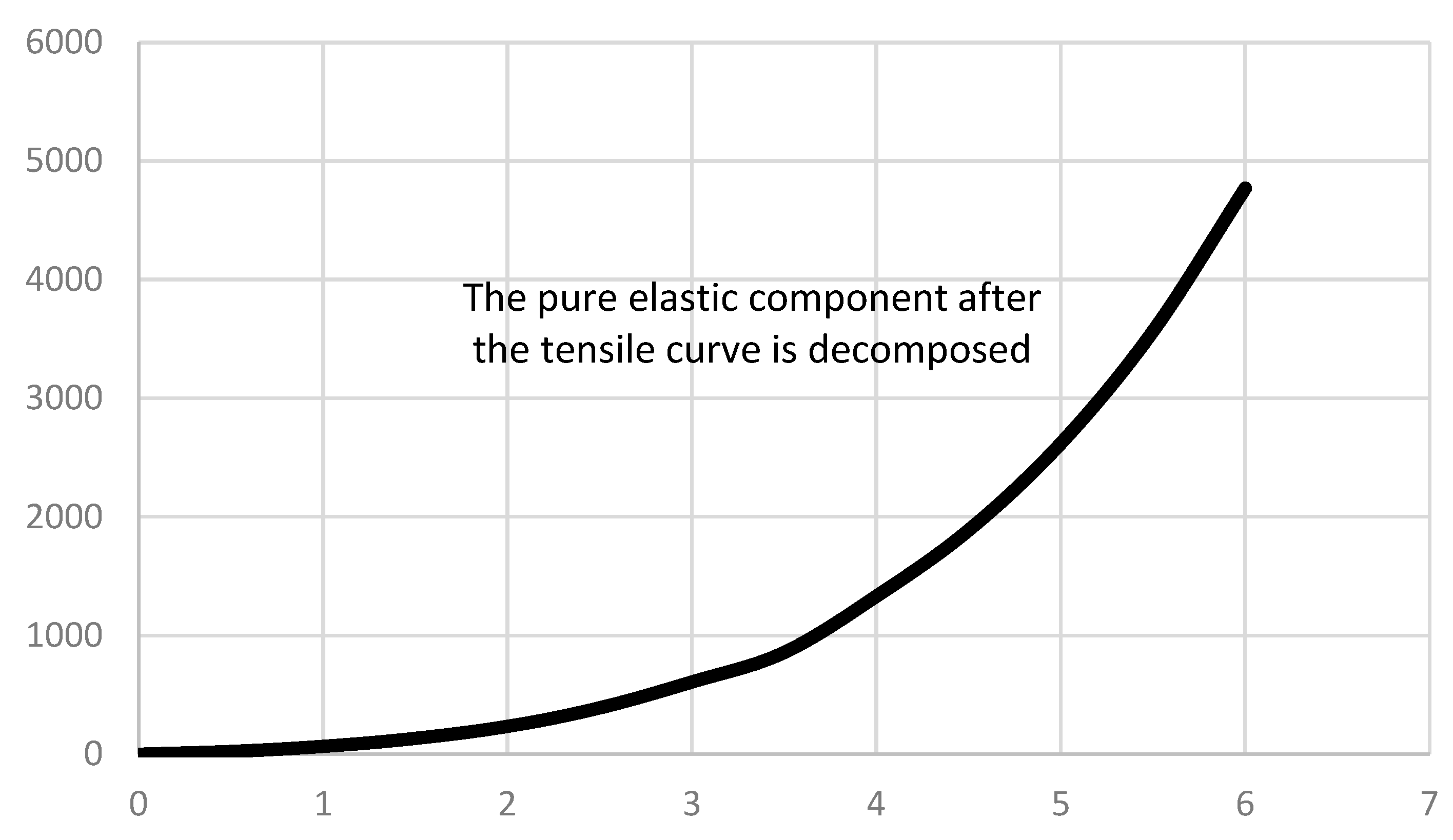
There is highly complex tensile property data of a certain fabric measured using a uniaxial fabric tensile instrument. Through machine learning algorithms, its nonlinear elastic and hysteresis components can be decomposed. Its nonlinear elastic component is shown in Figure 3. It requires fitting using a fifth-degree polynomial.
Figure 3.
Tensile pure elastic curve chart (the pure elastic component after the tensile curve is decomposed).
The length of the fabric sample is 50 mm, and the measured maximum elongation is 12%, which is 6 mm. Taking one data sample every 0.02 mm of extension produces a total of 301 samples. The sampled values are encoded using float quantization. Each float encoding occupies 32-bit binary length. The total memory length occupied by the binary encoding of the data is 9632 bits. The maximum number of data list output is 5000.0 mN/cm. If we maintain one significant digit after the decimal point and include decimal point, carriage return and line feed codes, each dataset uses approximately six ASCII encodings on average. The total binary encoding length is approximately 12,642 bits. Its algorithm is described as follows.
| def f(a,x):return x*(a[0] + x*(a[1] + x*(a[2] + x*(a[3] + x*a[4])))) for i in range (0,300):print(round(f([32.88,25.68,5.86,1.18,0.11], i*0.02),2)) |
The description length is 987 bits in total. Comparing the description length of the algorithm’s information content with the encoding length of the algorithm’s output shows that the information can be compressed effectively. If Shannon’s information entropy calculation is used, according to Equation (10), it is possible to obtain a higher data compression ratio.
If one sample is taken for every 0.01 mm of extension, the amount of data for the same curve is doubled, but the amount of algorithm information does not change. It can be concluded that during the fabric measurement process, within the measurement interval, when the density of the sampling points reaches a certain level, increasing the density of the sampling points does not help to obtain effective information. It would be useful and interesting to conduct a detailed analysis of Shannon’s information content of fabric instrument measurement data and explore effective data encoding and compression methods in a future paper.
4.3. The Relationship between Multivariate Polynomials, Nonlinearity, and Complexity
In this section, the elastic component Si of the fabric’s mechanical properties and the equivalent friction force fci of the hysteresis component form their own multivariate nonlinear relationships are being considered. To approximate nonlinear mechanical properties with multivariate relationships, multivariate polynomials are being used.
The conceptual definition of multivariate polynomials in advanced algebra is: Suppose P is a number field, x1, x2,…, xn are n words. The form is
where , k1, k2, …, kn are non-negative integers and are called a monomial. If two monomials have exactly the same powers of the same literal, they are said to be congeners. Similar items can be merged. The sum of some monomials is given using
It is called an n-ary polynomial, or simply a polynomial.
Suppose f (x, y) has continuous partial derivatives up to the fourth order in a certain neighborhood of the zero point, and (h, k) is any point in the neighborhood. Let us try to use a binary cubic polynomial fp (x, y) in approximating a binary nonlinear function f (x, y) near the zero point. Applying the third-order Taylor formula, we get
where Rn is called the Lagrangian remainder of the Taylor expansion. Expanding Equation (16) and sorting out the coefficients of each term, we can get
In a similar way, the relationship between the number of terms and the number and degree of variables after merging similar terms of an approximation polynomial can be obtained as follows:
As can be seen from Figure 4 and Table 1, multivariate nonlinear functions can be transformed into high-dimensional linear space for processing approximation. But as the number of variables and their degree of nonlinearity increases, the dimensions of the linear space must increase rapidly, leading to a disaster of dimensionality.
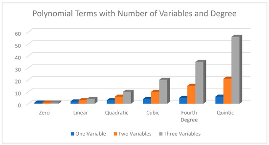
Figure 4.
Histogram of Table 1.

Table 1.
Relationships between the number of polynomial terms, the number of variables and the degree of the polynomial.
Description 6.
Let us describe a quadratic polynomial of two variables.
| def f(a,x,y):return a[0] + x*(a[1] + a[4]*y + x*a[3]) + y*(a[2] + a[5]*y) print(f([0.1021,0.4031,0.1257,0.2111,0.0101,0.1056],0.3505,0.8625)) |
The description length is 924 bits. A quadratic polynomial of two variables has the same number of terms as a quintic polynomial of one variable. Comparing Description 4, the complexity of describing quadratic polynomials of two variables is basically the same as that of quintic polynomials of one variable.
Description 7.
Let us now try to describe the cubic polynomial of two variables further.
| def f(a,x,y):return a[0]+x*(a[1]+a[4]*y+x*(a[3]+a[6]*x+a[7]*y))+y*(a[2]+y*(a[5]+a[8]*x+a[9]*y)) print(f([0.1011,0.3537,0.1257,0.2186,0.0101,0.1211,0.5433,0.1158,0.1358,0.3575],0.3505,0.8625)) |
The description length is 1344 bits.
Description 8.
The description of the ternary quadratic polynomial is as follows.
| def f(a,x,y,z):return a [0] + x*(a[1] + a[4]*x + a[5]*y + a[6]*z) + y*(a[2] + a[7]*y + a[8]*z) + z*(a[3] + a[9]*z) print(f([0.1011,0.3537,0.1257,0.2186,0.0101,0.1211,0.5433,0.1158,0.1358,0.3575],0.3505,0.8625,0.5708)) |
The number of terms in a cubic polynomial of two variables is also the same as the number of terms in a quadratic three-dimensional polynomial. Comparing Descriptions 7 and 8, shows that their description complexity is the same.
Comparing all descriptions except Description 5, we can conclude that the number of terms of a polynomial determines its complexity. The higher the number of terms in the polynomial, the higher the complexity.
We know that the number of terms of a polynomial depends on its number of variables and the nonlinearity of those variables. Multivariate variables and their nonlinear interactions generate a large number of cross-terms, rapidly increasing the number of terms in the polynomials that describe them.
When comparing the information loss caused by different fabric mechanics measurement and model reduction methods, we use fourth-order polynomials as a benchmark for comparison. In the third section of this paper, the number of main independent variables required for fabric measurement and modelling and their physical meanings have been determined. They exhibit cross-correlation on mechanical properties. The degree of nonlinearity of these fabrics cannot be determined until test data on the physical fabric is obtained. We empirically use the highest fifth-degree polynomial as their reference model. The number of terms in the final polynomial still needs to be determined using the machine learning algorithm from the measured data of the fabric in accordance with Occam’s razor principle. The statistical average of the degree of polynomial described using the degree of nonlinearity of mechanical properties is close to four degrees.
Description 9.
Use the cumulative integration method to describe the integral of the Dahl friction hysteresis model (Equation (16)).
| If (‘hs’ not in vars().keys()): hs = 0 def sgn(x): if (x < 0): return −1 else: return 1 def h(xgm,fc,ds): global hs hs = hs + xgm*(1 − sgn(ds)*hs/fc)*ds return hs print(h(0.8052,0.2035,0.1001)) |
The description length is 1323 bits. Contrast this with Description 7, which is close to the complexity of the polynomial description with 10 terms.
4.4. Complexity of Pure Elastic and Friction Hysteresis Components
It has been shown in Section 3 that although the physical meanings are different, the mathematical model descriptions of the equivalent friction force of the pure elastic component and the friction hysteresis component of the fabric’s mechanical properties are similar. Consequently, their Kolmogorov complexity is naturally the same. However, due to the path dependence of friction hysteresis, the equivalent friction force is only part of the description of friction hysteresis. After obtaining the equivalent friction force, the friction hysteresis still needs to be described using the extended pre-slip model such as Dahl (Description 9) and following up with integration on Dahl’s differential model. Therefore, the frictional hysteresis component has a higher Kolmogorov complexity than the purely elastic component. i.e., it generates a higher uncertainty in the fabric’s mechanical properties than the purely elastic component, confirming our earlier observations.
- In practical and theoretical research and engineering applications of fabric mechanics, the elastic component of mechanical properties has received more attention. This is because there is still limited awareness of the contribution of friction hysteresis’s high complexity to the mechanical properties of fabrics, and obtaining and effectively characterizing friction hysteresis information is difficult due to the high complexity of friction hysteresis.
Replacing the hysteresis caused by dry friction with the damping caused by internal friction in the fluid, which is different in physical meaning from friction hysteresis, and simplifying the characterization of friction hysteresis will cause the model or simulation to lose a lot of fabric mechanical information. Completely ignoring its existence will inevitably cause the model and simulation to lose more than 50% of the algorithm information.
4.5. Information Loss of Uniaxial Measurements and Models
Since the pioneering fabric mechanical measurement and research by (Haas & Dietzius, as reported by Yousef and Stylios, 2015), biaxial measurement technology of fabric mechanical properties has perplexed the industry [47]. It is difficult to obtain measurement data for fabric low-stress mechanical properties described using Equation (11). There is still no effective measurement method for the bending characteristics described using Equation (12). The difficulty of the measurement process and the lack of measurement methods have led to most measurements, models and simulations being reduced to relatively simple uniaxial methods.
But we need to understand the effects of this information loss using uniaxial measurements, models and simulations instead of corresponding multivariate nonlinear measurements and models. How much authenticity can such simulations of fabrics and clothing provide? Due to the nonlinear diversity of physical fabrics, such questions cannot be answered using simple sample comparison methods.
For fabric in-plane deformation, using uniaxial measurement, models and simulations, Equation (11) is simplified to
Taking the stress–strain relationship of in Equation (24) as an example, a fourth-order polynomial is chosen to meet the average requirement for describing the degree of nonlinearity of the fabric. The stress–strain relationship uses five polynomial terms to describe S1; five terms describe the equivalent friction force of friction hysteresis, and the complexity equivalent to ten polynomial terms describe the hysteresis model. A total complexity equivalent to twenty polynomial terms is used to describe the stress–strain relationship of . If Equation (11) is used to describe the stress–strain relationship of , under the same degree of fabric nonlinearity, thirty-five polynomial terms are needed to describe S1. Thirty-five terms describe the equivalent friction force of friction hysteresis, and an additional complexity equivalent to ten polynomial terms describes the hysteresis model. A total of eighty polynomial terms are required to describe the stress–strain relationship of . Uniaxial measurements and models retain only about a quarter of the information on mechanical properties. Even though this quarter of the information may be among the most important for the mechanical properties of the fabric, too much information loss will make the result of measurements and models deviate from reality.
The information loss due to the over-linearisation of nonlinear characteristics is an important consequence. If the nonlinear description ability of the model is reduced below the true nonlinearity of the fabric, the number of terms of the polynomial can be reduced, and the complexity of the model will be lost. For example, linear springs are used instead of nonlinear mapping relationships, and output results are less realistic, as is currently practised with CAD models used nowadays.
5. Conclusions and Outlook
Considering the challenges of fabric mechanics, this paper aims to establish how to precisely define the mechanical behaviour of fabrics as engineering materials using Komogorov complexity, offering a new way of thinking about measurements, models, and simulations. The paper aims to provide answers about the complexity of the frictional hysteresis component in fabric mechanics and whether it can be simplified or ignored. Recognising that most fabric mechanical data are produced through uniaxial measurements, how significant is the information loss, and finally, how we can compromise between model accuracy and computational complexity.
This paper shows that information theory and Kolmogorov complexity provide new ways of thinking about the nature and reality of measurements, models and simulations of fabric mechanics. A loss in the complexity (algorithmic information content) of measured, modelled, and simulated fabric mechanical properties will render their results significantly less realistic. Hence, through algorithm information analysis, the following conclusions can be drawn from this research:
- The frictional hysteresis component in fabric’s mechanical properties provides a higher level of complexity than the purely elastic component. This paper shows that ignoring the friction hysteresis component will cause the model and simulation to lose more than 50% of the algorithm information. For example, the pure elastic component and the Coulomb friction of a fabric need to be described using three-dimensional fourth-order polynomials. If the friction hysteresis component is ignored, we can have a 56% loss of information, and if there is a frictional overshoot, the loss of information will be even greater.
- Although uniaxial measurements are technically easier to implement than their multivariate counterparts, we have shown that an average loss of information can be as high as 75%. Hence, the vast number of models that use unary relationships to describe fabric behaviour and ignore the presence of frictional hysteresis are inaccurate because they hold less than 12% of real fabric mechanics data.
- Oversimplification of nonlinearities in models and simulations can also cause significant information loss. For example, in the same ternary relationship, if a fabric with a quartic polynomial description is simplified and described using a linear relationship, it can be calculated from Table 1 that it can lose a staggering 88% of its mechanical information.
- Our research also shows that the entropy of data obtained from fabric instrument measurements is not high, so we have shown that it can be significantly compressed to facilitate data management, exchange and use.
Consequently, using Kolmogorov complexity and Shannon’s information theory, we can conclude the low-stress mechanics of fibrous flexible materials as follows: The friction hysteresis component and the pure elastic component in the mechanical properties of fabrics coexist in the form of co-action lines and co-action points. Measurements cannot directly obtain them individually. Friction hysteresis has branches, that is, path dependence, which cannot be simply represented by a nonlinear polynomial relationship. In view of the high degree of complexity of friction hysteresis, which carries more than 50% of fabric’s mechanical information, an algorithm needs to be developed to decompose the friction hysteresis components and pure elastic components contained in the measurement data and to effectively characterize them.
The fabric instrument measurement technology has long posed challenges to the development of fabric mechanics. Uniaxial measurement methods cannot obtain sufficient information to truly characterise the mechanical behaviours of fabrics. It is of great significance to develop a biaxial measurement system suitable for clothing applications. To obtain maximum information from measurements, it is necessary to develop new sensor technology, analogue signal conditioning, information conversion and encoding, artificial intelligence calibration and inter-dimensional decoupling technology of multi-dimensional sensors and data fusion technology. They all form the basis for developing new biaxial measurement solutions.
A balance should be sought between the computational complexity of the algorithm and nonlinear simplification to keep the model with enough rules and knowledge that its output remains sufficiently accurate.
Efforts should be directed towards developing algorithms and systems for efficient processing, compression, encoding and management of fabric instrument measurement data.
Due to the high degree of complexity, increasing the amount of information required for fabric measurements, models and simulations will inevitably lead to realistic computability issues. How to overcome real computability problems through improved algorithms, hardware instruction acceleration, parallel computing and machine learning remains a challenging aspect in the engineering mechanics of fibrous flexible assemblies.
Regarding the multivariate nonlinear relationship of fabric mechanics, our research involves the highest three-dimensional nonlinear relationship. The deformation analysis of the fabric shows that it has a five-dimensional nonlinear relationship if no simplification is applied.
Author Contributions
Software, L.L.; validation, L.L.; formal analysis, L.L.; conceptualization, L.L. and G.K.S.; methodology, L.L. and G.K.S.; resources, G.K.S.; writing—original draft preparation, L.L.; writing—review and editing, G.K.S.; supervision, G.K.S.; project administration, G.K.S.; funding acquisition, G.K.S. All authors have read and agreed to the published version of the manuscript.
Funding
This research is funded by EPSRC FUNDING: Integration of CFD and CAE for design and Performance assessment of protective clothing, Grant No. DT/E011098/1.
Data Availability Statement
Data are contained within the article.
Conflicts of Interest
The authors declare no conflicts of interest.
References
- Stylios, G. Engineering, re-engineering and reverse engineering of textiles or textile genetic engineering. Int. J. Cloth. Sci. Technol. 1998, 10, 1. [Google Scholar] [CrossRef]
- Hearle, J.W.S. The challenge of changing from empirical craft to engineering design. Int. J. Cloth. Sci. Technol. 2004, 16, 141–152. [Google Scholar] [CrossRef]
- Uhlenkamp, J.-F.; Hauge, J.B.; Broda, E.; Lutjen, M.; Freitag, M.; Thoben, K.-D. Digital Twins: A Maturity Model for Their Classification and Evaluation. IEEE Access 2022, 10, 69605–69635. [Google Scholar] [CrossRef]
- Ngo, C.; Boivin, S. Nonlinear Cloth Simulation. [Research Report] RR-5099, INRIA. Ffinria-00071484. 2004. Available online: https://www.semanticscholar.org/paper/Nonlinear-Cloth-Simulation-Ngo-Boivin/986290a5499944618678c6e092a5e45894c4e3d5 (accessed on 1 January 2024).
- Stylios, G.K. Garment simulation. Int. J. Cloth. Sci. Technol. 2008, 20, 1. [Google Scholar] [CrossRef]
- Miguel, E.; Tamstorf, R.; Bradley, D.; Schvartzman, S.; Thomaszewski, B.; Bickel, B.; Matusik, W.; Marschner, S.; Otaduy, M. Modeling and Estimation of Internal Friction in Cloth. ACM Trans. Graph. 2013, 32, 212. [Google Scholar] [CrossRef]
- Volino, P.; Magnenat-Thalmann, N.; Faure, F. A simple approach to nonlinear tensile stiffness for accurate cloth simulation. ACM Trans. Graph. 2009, 28, 105. [Google Scholar] [CrossRef]
- Wang, H.; O’Brien, J.; Ramamoorthi, R. Data-driven elastic models for cloth. ACM Trans. Graph. 2011, 30, 71. [Google Scholar] [CrossRef]
- Wang, M.; Wang, M.; Li, X. Study on improving three-dimensional dynamic simulation model and equation of flexible fabric. Adv. Mech. Eng. 2019, 11, 1–6. [Google Scholar] [CrossRef]
- Sun, F.; Hu, X. Effect of meso-scale structures and hyperviscoelastic mechanics on the nonlinear tensile stability and hysteresis of woven materials. Mater. Res. Express 2020, 7, 075306. [Google Scholar] [CrossRef]
- Stylios, G.K.; Wan, T.R.; Powell, N.J. Modelling the dynamic drape of garments on synthetic humans in a virtual fashion show. Int. J. Cloth. Sci. Technol. 1996, 8, 95–112. [Google Scholar] [CrossRef]
- Chen, Y.; Wang, Q.J.; Zhang, M. Accurate simulation of draped fabric sheets with nonlinear modeling. Text Res. J. 2022, 92, 539–560. [Google Scholar] [CrossRef]
- Barbieri, M. What is information? Philosophical transactions of the Royal Society of London. Ser. A Math. Phys. Eng. Sci. 2016, 374, 1–10. [Google Scholar] [CrossRef]
- Rocchi, P. What is Information: Beyond the Jungle of Information Theories. Comput. J. 2012, 55, 856–860. [Google Scholar] [CrossRef]
- Wiener, N. Cybernetics or Control and Communication in the Animal and the Machine; John Wiley: Hoboken, NJ, USA, 1948. [Google Scholar]
- Adriaans, P. The Stanford Encyclopedia of Philosophy (Fall 2020 Edition); Zalta, E.N., Ed.; Pub. Metaphysics Research Lab, Stanford University: Stanford, CA, USA, 2021; Available online: https://plato.stanford.edu/archives/fall2020/entries/information/ (accessed on 1 January 2024).
- Sommaruga, G.; Kanade, T.; Kittler, J. Philosophical Conceptions of Information. In Formal Theories of Information; Springer: Berlin/Heidelberg, Germany, 2009. [Google Scholar]
- Shannon, C. The lattice theory of information. Trans. I.R.E. Prof. Group Inf. Theory 1953, 1, 105–107. [Google Scholar] [CrossRef]
- Nyquist, H. Certain factors affecting telegraph speed. Trans. Am. Inst. Electr. Eng. 1924, 43, 1197–1198. [Google Scholar] [CrossRef]
- Fisher, R.A. Statistical Methods for Research Workers, 11th ed.; Oliver and Boyd: Edinburgh, UK, 1925. [Google Scholar]
- Hartley, R.V.L. Transmission of Information 1. Bell Syst. Tech. J. 1928, 7, 535–563. [Google Scholar] [CrossRef]
- Shannon, C.E. A Mathematical Theory of Communication. Bell Syst. Tech. J. 1948, 27, 379–423. [Google Scholar] [CrossRef]
- Kolmogorov, A.N. On Tables of Random Numbers. Sankhya Ser. A 1963, 25, 369–376. [Google Scholar] [CrossRef]
- Kolmogorov, A.N. Three approaches to the quantitative definition of information. Int. J. Comput. Math. 1968, 2, 157–168. [Google Scholar] [CrossRef]
- Kolmogorov, A.N. Logical basis for information theory and probability theory. IEEE Trans. Inf. Theory 1968, 14, 662–664. [Google Scholar] [CrossRef]
- Solomonoff, R.J. A Preliminary Report on a General Theory of Inductive Inference; Zator Company: Cambridge, MA, USA, 1960. [Google Scholar]
- Solomonoff, R.J. A formal theory of inductive inference. Part I. Inf. Control 1964, 7, 1–22. [Google Scholar] [CrossRef]
- Solomonoff, R.J. A formal theory of inductive inference. Part II. Inf. Control 1964, 7, 224–254. [Google Scholar] [CrossRef]
- Chaitin, G. On the Simplicity and Speed of Programs for Computing Infinite Sets of Natural Numbers. J. ACM 1969, 16, 407–422. [Google Scholar] [CrossRef]
- Turing, A.M. On Computable Numbers, with an Application to the Entscheidungsproblem. Proc. Lond. Math. Soc. 1937, s2-42, 230–265. [Google Scholar] [CrossRef]
- Li, M. An Introduction to Kolmogorov Complexity and Its Applications, 4th ed.; Springer Nature: Cham, Switzerland, 2019. [Google Scholar] [CrossRef]
- Cover, T.M.; Thomas, J.A. Elements of Information Theory; Wiley Series in Telecommunications and Signal Processing; Wiley-Interscience: Hoboken, NJ, USA, 2006. [Google Scholar]
- Postle, R. Fabric objective measurement technology: Present status and future potential. Int. J. Cloth. Sci. Technol. 1990, 2, 7–17. [Google Scholar] [CrossRef]
- Stylios, G. (Ed.) Textile Objective Measurement and Automation in Garment Manufacture; Ellis Horwood Ltd.: London, UK, 1991; 282p, ISBN 10 0139127429; 13 978-0139127427. [Google Scholar]
- Kawabata, S.; Niwa, M.; Kawai, H. 3-the finite-deformation theory of plain-weave fabrics part i: The biaxial-deformation theory. J. Text. Inst. 1973, 64, 21–46. [Google Scholar] [CrossRef]
- Kawabata, S.; Niwa, M.; Kawai, H. 4-the finite-deformation theory of plain-weave fabrics. part ii: The uniaxial-deformation theory. J. Text. Inst. 1973, 64, 47–61. [Google Scholar] [CrossRef]
- Hu, J. Structure and Mechanics of Woven Fabrics; Elsevier Science: Cambridge, MA, USA, 2004. [Google Scholar] [CrossRef]
- Kawabata, S.; Niwa, M.; Kawai, H. 5-the finite-deformation theory of plain-weave fabrics. part iii: The shear-deformation theory. J. Text. Inst. 1973, 64, 62–85. [Google Scholar] [CrossRef]
- Gupta, B.S. Textile fiber morphology, structure and properties in relation to friction. Woodhead Publishing. Frict. Text. Mater. 2008, 88, 3–36. [Google Scholar] [CrossRef]
- Yousef, M.I.; Stylios, G.K. Investigating the challenges of measuring combination mechanics in textile fabrics. Text. Res. J. 2018, 88, 2741–2754. [Google Scholar] [CrossRef]
- Dahl, P.R. A Solid Friction Model; TOR-0158 (3107-18-1); The Aerospace Corporation: El Segundo, CA, USA, 1968. [Google Scholar]
- Bliman, P. Mathematical study of the Dahl’s friction model. Eur. J. Mech. A-Solids 1992, 11, 835–848. [Google Scholar]
- Bliman, P.A.; Sorine, M. Friction Modeling by Hysteresis Operators. Application to Dahl, Sticktion, and Stribeck Effects. Models of Hysteresis; Longman Scientific and Technical: London, UK, 1993. [Google Scholar]
- Bliman, P.A.; Sorine, M. A System-Theoretic Approach of Systems with Hysteresis. Application to Friction Modelling and Compensation. In Proceedings of the 2nd European Control Conference, Gronigen, The Netherlands, 28 June–1 July 1993; pp. 1844–1849. [Google Scholar]
- Bliman, P.A.; Sorine, M. Easy-to-Use Realistic Dry Friction Models for Automatic Control. In Proceedings of the 3rd European Control Conference, Rome, Italy, 5–8 September 1995; pp. 3788–3794. [Google Scholar]
- Weierstrass, K. Über die analytische Darstellbarkeit sogenannter willkürlicher Functionen einer reellen Veränderlichen. Sitzungsberichte Der Königlich Preußischen Akad. Der Wiss. Zu Berl. 1885, II, 633–639. [Google Scholar]
- Yousef, M.I.; Stylios, G.K. Legacy of the Zeppelins: defining fabrics as engineering materials. J. Text. Inst. 2015, 106, 480–489. [Google Scholar] [CrossRef]

Disclaimer/Publisher’s Note: The statements, opinions and data contained in all publications are solely those of the individual author(s) and contributor(s) and not of MDPI and/or the editor(s). MDPI and/or the editor(s) disclaim responsibility for any injury to people or property resulting from any ideas, methods, instructions or products referred to in the content. |
© 2024 by the authors. Licensee MDPI, Basel, Switzerland. This article is an open access article distributed under the terms and conditions of the Creative Commons Attribution (CC BY) license (https://creativecommons.org/licenses/by/4.0/).