Article

Climate Change and Soil Health: Explainable Artificial Intelligence Reveals Microbiome Response to Warming

by
Pierfrancesco Novielli
1,2,†,
Michele Magarelli
1,†,
Donato Romano
1,2,
Lorenzo de Trizio
1,
Pierpaolo Di Bitonto
1,
Alfonso Monaco
2,3,
Nicola Amoroso
2,4,
Anna Maria Stellacci
1,
Claudia Zoani
5,
Roberto Bellotti
2,3 and
Sabina Tangaro
1,2,*
1
Dipartimento di Scienze del Suolo, della Pianta e degli Alimenti, Università degli Studi di Bari Aldo Moro, 70125 Bari, Italy
2
Istituto Nazionale di Fisica Nucleare, Sezione di Bari, 70125 Bari, Italy
3
Dipartimento Interateneo di Fisica “M. Merlin”, Università degli Studi di Bari Aldo Moro, 70125 Bari, Italy
4
Dipartimento di Farmacia-Scienze del Farmaco, Università degli Studi di Bari Aldo Moro, 70125 Bari, Italy
5
Dipartimento Sostenibilità, Circolarità e Adattamento al Cambiamento Climatico dei Sistemi Produttivi e Territoriali, Divisione Biotecnologie e Agroindustria—ENEA, C.R. Casaccia, 00123 Rome, Italy
*
Author to whom correspondence should be addressed.
These authors contributed equally to this work.
Mach. Learn. Knowl. Extr. 2024, 6(3), 1564-1578; https://doi.org/10.3390/make6030075
Submission received: 13 May 2024 / Revised: 5 July 2024 / Accepted: 7 July 2024 / Published: 10 July 2024
(This article belongs to the Section Learning)

Abstract

:
Climate change presents an unprecedented global challenge, demanding collective action to both mitigate its effects and adapt to its consequences. Soil health and function are profoundly impacted by climate change, particularly evident in the sensitivity of soil microbial respiration to warming, known as Q10. Q10 measures the rate of microbial respiration’s increase with a temperature rise of 10 degrees Celsius, playing a pivotal role in understanding soil carbon dynamics in response to climate change. Leveraging machine learning techniques, particularly explainable artificial intelligence (XAI), offers a promising avenue to analyze complex data and identify biomarkers crucial for developing innovative climate change mitigation strategies. This research aims to evaluate the extent to which chemical, physical, and microbiological soil characteristics are associated with high or low Q10 values, utilizing XAI approaches. The Extra Trees Classifier algorithm was employed, yielding an average accuracy of 0.923 ± 0.009 , an average AUCROC of 0.964 ± 0.004 , and an average AUCPRC of 0.963 ± 0.006 . Additionally, through XAI techniques, we elucidate the significant features contributing to the prediction of Q10 classes. The XAI analysis shows that the temperature sensitivity of soil respiration increases with microbiome variables but decreases with non-microbiome variables beyond a threshold. Our findings underscore the critical role of the soil microbiome in predicting soil Q10 dynamics, providing valuable insights for developing targeted climate change mitigation strategies.

1. Introduction

Global warming represents one of the most urgent challenges humanity faces today. This phenomenon is primarily attributed to the increase in greenhouse gas emissions into the atmosphere, caused by human activities such as the use of fossil fuels, deforestation, and other industrial activities. Climate change has a significant impact on soil health and function [1,2,3]. Climate change can lead to modifications in temperature regimes and precipitation patterns, directly influencing soil temperature and water availability. These changes can affect the distribution of soil microbial communities and the processes of organic matter decomposition. Rising temperatures can accelerate the processes of organic matter decomposition in the soil, increasing emissions of greenhouse gases such as carbon dioxide (CO2) and methane (CH4) [4] and leading to a decline in soil quality and health. Climate changes can affect agricultural production and the availability of food resources, risking food security for millions of people worldwide. Today, numerous studies highlight the significant impact of nutrient transmission or contaminant from the soil to people, and how the health of the soil, particularly in the face of increasing exposure to environmental pollutants and pathogens, influences the availability and safety of food. If the soil is contaminated with harmful chemicals, such as pesticides, herbicides, heavy metals, or other pollutants, these substances can be absorbed by plants and transferred to consumers through food. Exposure to such chemicals can have harmful effects on human health. A healthy soil also acts as a natural filter for air and water. Plants absorb atmospheric pollutants and filter rainwater, contributing to maintaining a clean and healthy environment for humans and surrounding ecosystems [5]. Changes in temperatures and precipitation patterns can influence crop growth, increase the risk of plant diseases, and reduce agricultural yields. The soil microbiota represents the focal point of the discourse when it comes to understanding the impact of climate change on terrestrial ecosystems. The soil microbiome, comprising diverse microorganisms, such as bacteria, fungi, viruses, archaea, and unicellular organisms, plays a fundamental role in soil ecosystems. This complex community influences soil fertility, plant health, and food production. Moreover, soil microorganisms contribute to the decomposition of organic matter and the release of essential nutrients, influencing plant growth, crop yield, and food quality. Microbial respiration breaks down organic matter in soil through the consumption of oxygen and the release of carbon dioxide (CO2) as a byproduct and it plays a crucial role in the cycling of carbon and nutrients in terrestrial ecosystems [6]. During microbial respiration, microorganisms utilize organic substrates, such as plant residues, root exudates, and other organic matter, as energy sources to fuel their metabolic activities. As they respire, they oxidize these organic compounds, releasing CO2 into the soil atmosphere. Microbial respiration is influenced by various environmental factors, including temperature, moisture, pH, nutrient availability, and substrate quality and degradability [7]. Warmer temperatures generally accelerate microbial activity and respiration rates, while water availability and substrate quality also play important roles in regulating microbial respiration rates. The sensitivity of soil microbial respiration to warming, often referred to as Q10, is a measure of how much the rate of microbial respiration in soil increases with a temperature increase of 10 °C [8]. It is a crucial parameter in understanding the response of soil carbon dynamics to climate change. A higher Q10 value indicates that soil microbial respiration is more sensitive to temperature changes, meaning that a small increase in temperature leads to a relatively larger increase in respiration rate. Conversely, a lower Q10 value suggests less sensitivity to temperature changes. Understanding the Q10 value helps scientists predict how soil carbon stocks may respond to future climate warming scenarios and inform climate change mitigation and adaptation strategies. To effectively address this challenge, concerted efforts on a global scale are needed to reduce greenhouse gas emissions, adopt renewable energy sources, improve energy efficiency, protect ecosystems, and adapt to ongoing climate change. Machine learning (ML) methods can play a significant role in contributing to efforts to address climate change and global warming [9,10,11] by providing tools and techniques to analyze complex data, make predictions [12,13,14], and develop innovative solutions to mitigate the effects of climate change. In our analysis, we utilized soil characteristics to predict the sensitivity of soil microbial respiration to warming (Q10). The study of extreme classes has often been instrumental in identifying biomarkers of a phenomenon and understanding its dynamics. For instance, in medicine, the discrimination between healthy and diseased states aims precisely at pinpointing disease biomarkers. Explainable artificial intelligence-based models play a pivotal role in achieving this objective, as they enable the identification of biomarkers through multivariate analysis.
Our primary objective was to discern the key soil factors that differentiate between soils exhibiting low Q10 values and those with high Q10 values. To achieve this, we segmented the Q10 values into two extreme classes: one comprising samples falling below the 25th percentile and the other above the 75th percentile. We then employed an ML classifier to predict this binary categorization. Subsequently, we implemented an explainable artificial intelligence (XAI) strategy to gain insights into how the classification model makes predictions, thereby facilitating the determination of feature importance. With XAI, we can discern the individual contribution of each variable for every soil sample. Specifically, leveraging algorithms like SHapley Additive exPlanations (SHAP), a model-agnostic post hoc method, enables us to interpret prediction results on a localized level [15]. This means we can understand how each variable influences the prediction outcome for each specific soil sample, providing granular insights into the underlying mechanisms driving soil respiration sensitivity to warming [16,17].
Using XAI is crucial in this study because it enhances the transparency and interpretability of the machine learning model, which is often criticized for being a “black box”. While XAI has been extensively used in various fields, its application to understanding soil microbial respiration sensitivity to warming (Q10) is novel. By utilizing XAI, we provide an unprecedented level of transparency and interpretability in this specific context, which is crucial for understanding and mitigating climate change impacts on soil ecosystems. Our study integrates a wide range of soil characteristics, including chemical, physical, and microbiological properties, alongside environmental and land-use variables. This comprehensive approach allows us to explore complex interactions and their impact on Q10, providing a holistic understanding that extends beyond traditional univariate analyses. By centering our analysis around XAI, we bridge the gap between complex machine learning models and domain experts in soil science and climate change. This approach not only enhances the validity of our findings but also makes them more accessible and actionable for experts of the field.
Our approach aims to contribute to a comprehensive understanding of the relationships between the Q10 value and soil (chemical, physical, and microbiological properties), environmental, and land use variables, particularly the composition of the microbiome. Given the urgent need to address global warming, it is essential to take concrete actions on a global scale to reduce greenhouse gas emissions to protect ecosystems, and adapt to ongoing climate change. Our work exemplifies the application of machine learning and XAI to a real-world problem, highlighting the broader applicability and impact of these methods. This interdisciplinary approach is crucial for advancing both environmental science and machine learning.
The structure of this paper is as follows: Section 2 provides a detailed description of the materials and methods used in the analysis, including the machine learning algorithms employed. Subsequently, Section 3 presents the results obtained in terms of predictive outcomes and XAI analysis. The discussion of the results is carried out in Section 4, and finally, Section 5 encapsulates the conclusions drawn from the study.

2. Materials and Methods

The data used in this study, as described in Table 1, were downloaded from a public repository where a global survey had been conducted across 332 samples collected over 29 countries [18]. These samples represent locations from 29 countries, offering a comprehensive overview of diverse climatic conditions and soil properties worldwide. The dataset includes a wide range of environmental factors, such as the mean annual temperature (MAT) ranging from −7 °C to 30 °C, as well as various vegetation types and soil properties. For each soil sample, 27 factors of a different nature were identified, covering environmental, soil microbiota, biochemical recalcitrance, substrate quantity, and mineral protection factors. Each soil sample is associated with a Q10 value, providing comprehensive insights into soil respiration sensitivity to warming. This information is organized in a tabular format, where each row corresponds to a specific sample, and each column represents a distinct soil characteristic. Environmental factors includes soil variables (chemical, physical characteristics), land use, meteorological variables and location of the sampling site, and specifically, longitude, presence of forest, mean annual precipitation (MAP), mean annual temperature (MAT), plant richness, plant cover, pH, electrical conductivity, percentage of clay + silt, soil total phosphorus, and soil C:N ratio based on total organic carbon and total N [19]. Biochemical recalcitrance includes the percentage of aromatic, percentage of alkane, percentage of polysaccharide, and percentage of amide. Mineral protection includes the proportion of particulate organic C and the proportion of mineral-associated organic C ratio. Finally, the soil microbiome [20] includes mean glucose-induced soil respiration, serving as an indicator of the total microbial biomass, richness of bacteria, richness of fungi, richness of protists, standardized proportion of bacteria taxa negatively associated with Q10, standardized proportion of fungi taxa negatively associated with Q10, standardized proportion of protist taxa negatively associated with Q10, standardized proportion of bacteria taxa positively associated with Q10, standardized proportion of fungi taxa positively associated with Q10, and the standardized proportion of protist taxa positively associated with Q10.

2.1. Data Preparation

In order to evaluate the most influential factors distinguishing soils with high and low Q10 values, we partitioned the soil samples into two categories, a common approach for categorizing a continuous variable [21]. Soils with low Q10 values were classified as those falling below the 25th percentile, while those with high Q10 values were classified as those above the 75th percentile. Consequently, we obtained a dataset consisting of 83 soils with low Q10 values and 83 soils with high Q10 values.
For our analysis, we considered all available environmental, microbiome [22], and biochemical variables. The data were standardized to ensure that each variable had a mean of 0 and a variance of 1 [23].

2.2. Machine Learning-Based Classification

Figure 1 illustrates the workflow adopted for the analysis. The histogram of the Q10 variable, segmented into high and low Q10 categories, provides an initial insight into the distribution of the data. Subsequently, all variables associated with these soils were merged, forming the input table for the explainable artificial intelligence (XAI) framework.
To ensure the stability and robustness of our findings, a nested cross-validation procedure (K = 10) was conducted, repeated 20 times. During this process, the machine learning algorithm parameters were tuned within the inner cross-validation loop. Following this, SHAP (SHapley Additive exPlanations) values were computed to enhance transparency and elucidate the importance and direction of variable effects.
To evaluate the performance of various machine learning models for predicting high and low Q10 values, we conducted a comprehensive comparison involving several classifiers, including ensemble methods, Decision Tree, Support Vector Machine (SVM), K-Nearest Neighbors (KNN), and Logistic Regression. For each model, we performed hyperparameter tuning to optimize their performance.
Support Vector Machines are powerful classifiers known for their effectiveness in high-dimensional spaces. The SVM algorithm constructs a hyperplane or set of hyperplanes in a high-dimensional space to separate different classes. We experimented with different kernels (linear, polynomial, radial basis function, and sigmoid) and regularization parameters to optimize the model’s performance [24]. The hyperparameters for SVM were tuned using the following grid:
  • C ∈ {1.0, 0.1, 0.01, 0.5},
  • kernel ∈ {‘linear’, ‘poly’, ‘rbf’, ‘sigmoid’}.
The K-Nearest Neighbors algorithm is a non-parametric method used for classification. It classifies a data point based on the majority class of its neighbors. We evaluated the model using different numbers of neighbors, distance metrics, and weight functions [25]. The hyperparameters for KNN were tuned using the following grid:
  • n_neighbors ∈ {3, 5, 7, 9, 11},
  • weights ∈ {‘uniform’, ‘distance’},
  • metric ∈ {‘euclidean’, ‘manhattan’}.
Logistic Regression is a linear model used for binary classification that predicts the probability of a class label based on one or more predictor variables. We tuned several parameters, including the regularization strength, penalty types, and solvers. Additionally, we considered the elastic net penalty, which is a combination of L1 and L2 penalties, to improve model performance by handling multicollinearity and selecting relevant features [26]. The hyperparameters for Logistic Regression were tuned using the following grid:
  • penalty ∈ {‘l1’,‘l2’,‘elasticnet’},
  • C ∈ {1.0, 0.1, 0.01, 0.5},
  • solver ∈ {‘lbfgs’, ‘liblinear’, ‘saga’}.
The Decision Tree (DT) Classifier is a versatile, non-parametric supervised learning technique employed for both classification and regression tasks. The objective is to develop a model that forecasts the value of a target variable by deriving straightforward decision rules from the data features. The structure of a decision tree is hierarchical and tree-like, comprising a root node, branches, internal nodes, and leaf nodes [27]. The hyperparameters for Decision Tree were tuned using the following grid:
  • max_depth ∈ {None, 3, 5, 7, 9},
  • criterion ∈ { ‘gini’, ‘entropy’, ‘log_loss’}.
The Random Forest classifier is a machine learning algorithm, which combines multiple individual models to create a stronger, more accurate model. Random Forest is composed of a collection of decision trees. Each decision tree is built using a subset of the training data and a random selection of features. It uses a technique called bootstrapping, which creates multiple random subsets of the training data through sampling with replacement. Each subset is used to train a separate decision tree. At each node of the decision tree, instead of considering all features to make a split, Random Forest randomly selects a subset of features. This helps to decorrelate the trees and make them less sensitive to noise in the data. Random Forest combines the predictions of multiple trees, reducing overfitting and improving generalization performance [28].
The Extra Trees Classifier is an ensemble machine learning algorithm used for classification tasks. It belongs to the category of decision tree-based methods and leverages randomization to improve performance and reduce variance. Like other ensemble algorithms, the Extra Trees Classifier builds a set of decision trees. Each tree is trained on a random subset of the training data and uses random feature selection to split the nodes. Thanks to the randomization of split nodes and the use of random subsets of the training data, the Extra Trees Classifier tends to be less susceptible to overfitting compared to traditional decision trees. This makes it particularly useful in situations where data has a high degree of noise or variance. Extra Trees can effectively handle datasets with a large number of features, making it suitable for complex problems. Finally, the feature selection process during tree building allows for estimating the importance of each feature in the model [29].
XGBoost, abbreviated from “eXtreme Gradient Boosting,” stands as a widely utilized machine learning algorithm acclaimed for its proficiency in tackling regression and classification tasks. Renowned for its prowess in data science and machine learning competitions, XGBoost excels in delivering outstanding performance across diverse problem domains and datasets. Its reputation for flexibility and scalability renders it indispensable for handling large volumes of data [30]. As an ensemble learning method, XGBoost represents an advancement over traditional gradient boosting algorithms. By constructing an ensemble of decision trees, with each tree contributing to the final prediction, XGBoost amplifies the model’s predictive prowess. Its built-in cross-validation functionality facilitates robust model evaluation and parameter tuning, ensuring optimal performance. Moreover, XGBoost’s ensemble approach, wherein models correct each other’s errors, engenders heightened predictive accuracy compared to many other algorithms. Additionally, the incorporation of regularization techniques addresses the challenge of overfitting, thereby ensuring the model’s adaptability to new data [31].
The parameters grid for the ensemble models is as follows:
  • max_depth ∈ {None, 3, 5, 7, 9},
  • n_estimators ∈ {50, 100, 150, 200, 250}.
By systematically exploring different values for these parameters, we sought to enhance the classifiers’ ability to generalize to unseen data and improve overall predictive accuracy.
Evaluation metrics are crucial tools for assessing the performance and effectiveness of machine learning models [32]. These metrics provide quantitative measures that help quantify how well a model is performing on a given task. The most commonly used evaluation metrics in classification analysis are:
  • Accuracy:
    The proportion of correctly classified instances among the total instances
    A C C = T P + T N T P + F P + T N + F N
  • Area Under the ROC Curve (AUC-ROC):
    The ROC (Receiver Operating Characteristic) curve and AUC (Area Under the Curve) are assessment tools employed to gauge the effectiveness of a binary classification model. The ROC curve presents a graphical depiction of how sensitivity (true positives) and specificity (true negatives) change across various classification thresholds. Essentially, it illustrates the balance between accurately identifying positive and negative instances by the model. The AUC quantifies the overall performance of the model by measuring the area under the ROC curve: a value closer to 1 signifies superior model performance, while a value around 0.5 suggests random classification. In summary, these metrics are vital for evaluating and contrasting the classification ability of binary models [33].
  • Area Under the PRC Curve (AUC-PRC):
    The Precision-Recall Curve (PRC) and Area Under the Curve (AUC) are tools used to evaluate the performance of a binary classification model. The PRC represents the relationship between precision (true positive rate) and recall (sensitivity) of the model at different decision thresholds. Precision measures the fraction of instances classified as positive that are actually positive, while recall measures the fraction of actual positive instances in the dataset that are correctly identified by the model. The Area Under the PRC Curve provides an aggregated measure of the model’s performance in terms of precision and recall. A larger area indicates better performance, with a maximum area of 1 corresponding to a perfect model [34].

2.3. Explainable Artificial Intelligence (XAI)

Explainable Artificial Intelligence (XAI) stands as a pivotal advancement in AI systems, ensuring that models remain interpretable and comprehensible to humans. Within XAI, two prominent methods are commonly employed: SHapley Additive exPlanations (SHAP) and feature importance [35].
SHapley Additive exPlanations (SHAP) offers a methodological approach to elucidate the outputs of machine learning models by attributing significance to each feature with respect to the model’s predictions. By quantifying the impact of individual features on predictions, SHAP values provide valuable insights into the reasoning behind model outcomes [36].
The SHAP value for the jth feature of the instance x is calculated by aggregating it across all possible subsets according to the formula:
Φ j ( x ) = F S { j } | F | ! ( | S | | F | 1 ) ! | S | ! [ f x ( F j ) f x ( F ) ]
Here, | F | ! denotes the permutations of features in the subset F, ( | S | | F | 1 ) ! represents the permutations of features in the subset S ( F { j } ) , and | S | ! signifies the total number of feature permutations.
Feature importance serves as a technique aimed at discerning the most influential features within a machine learning model. By ranking features based on their contribution to model performance, feature importance aids in prioritizing features for further analysis and decision-making. Notably, tree-based machine learning models inherently embed feature importance metrics.

3. Results

The objective of this research was to assess, utilizing interpretable machine learning models, the extent to which biochemical, microbiome, and environmental soil characteristics are associated with higher or lower Q10 values. Table 2 presents the average performance of the ML classifiers, calculated as the mean performance obtained during the 10-fold cross-validation repeated 20 times. This approach was chosen to ensure the robustness of the machine learning model.
The results in Table 2 indicate that ensemble methods, specifically Extra Trees, Random Forest, and XGBoost, generally outperform other classifiers in terms of accuracy and AUC. The Extra Trees classifier achieved the highest accuracy (0.923 ± 0.009), AUROC (0.964 ± 0.004), and AUPRC (0.963 ± 0.006), demonstrating superior performance in distinguishing between the two classes. This can be attributed to the fact that ensemble methods aggregate predictions from multiple decision trees, thus reducing variance and mitigating overfitting. Non-ensemble methods, such as Decision Tree, SVM, KNN, and Logistic Regression, exhibited relatively lower performance. The Decision Tree classifier had the lowest accuracy (0.838 ± 0.022), AUROC (0.862 ± 0.027), and AUPRC (0.861 ± 0.031). This suggests that single decision trees are more prone to overfitting and less capable of capturing complex patterns in the data.
For further analysis, we showcase the XAI results of the best classifier, although similar behaviors are observed in the other models.
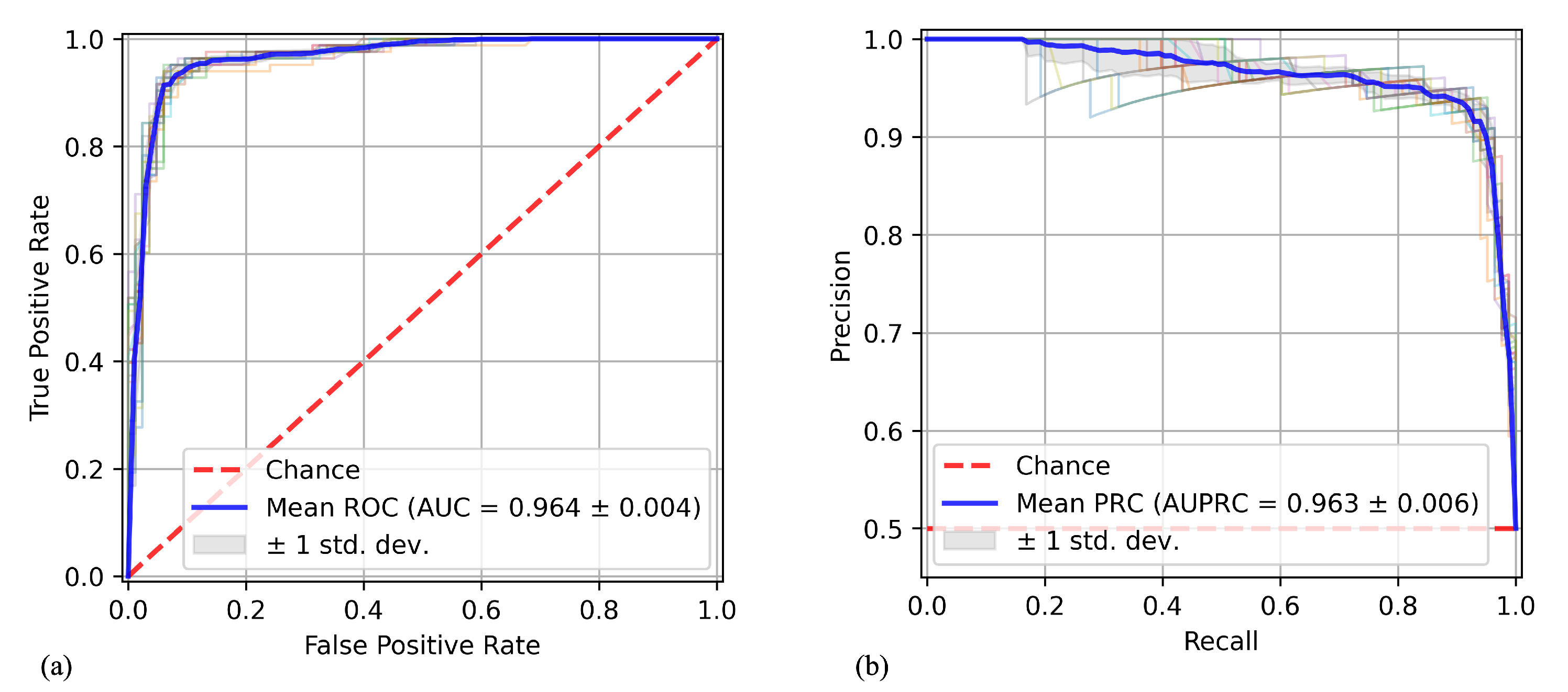
The average ROC is illustrated in Figure 2a. Each iteration of the cross-validation procedure yielded a unique AUC score, enabling the computation of the aggregate AUC across all iterations to evaluate the model’s comprehensive performance. Additionally, the Precision-Recall Curve (PRC) was computed, as depicted in Figure 2b.
Figure 3 represents the global feature importance obtained with the embedded feature importance from the ML model (Figure 3a) and the feature importance calculated with SHAP (Figure 3b). Feature importance methods aim to quantify the contribution of each feature to the model’s predictions. Global methods provide an overarching ranking of features, while local methods illuminate the contribution of each feature to a specific prediction.
For both feature importance techniques, the two most important variables are consistently the proportion of bacteria taxa positively associated with Q10 (“Bacteria_Positive”) and the glucose-induced soil respiration (“Mean_Glucose”). SHAP values, depicted in Figure 3b, construct interpretable linear models around each test instance and estimate feature importance at the local level. The plot reveals the most critical features for classification according to the SHAP algorithm.
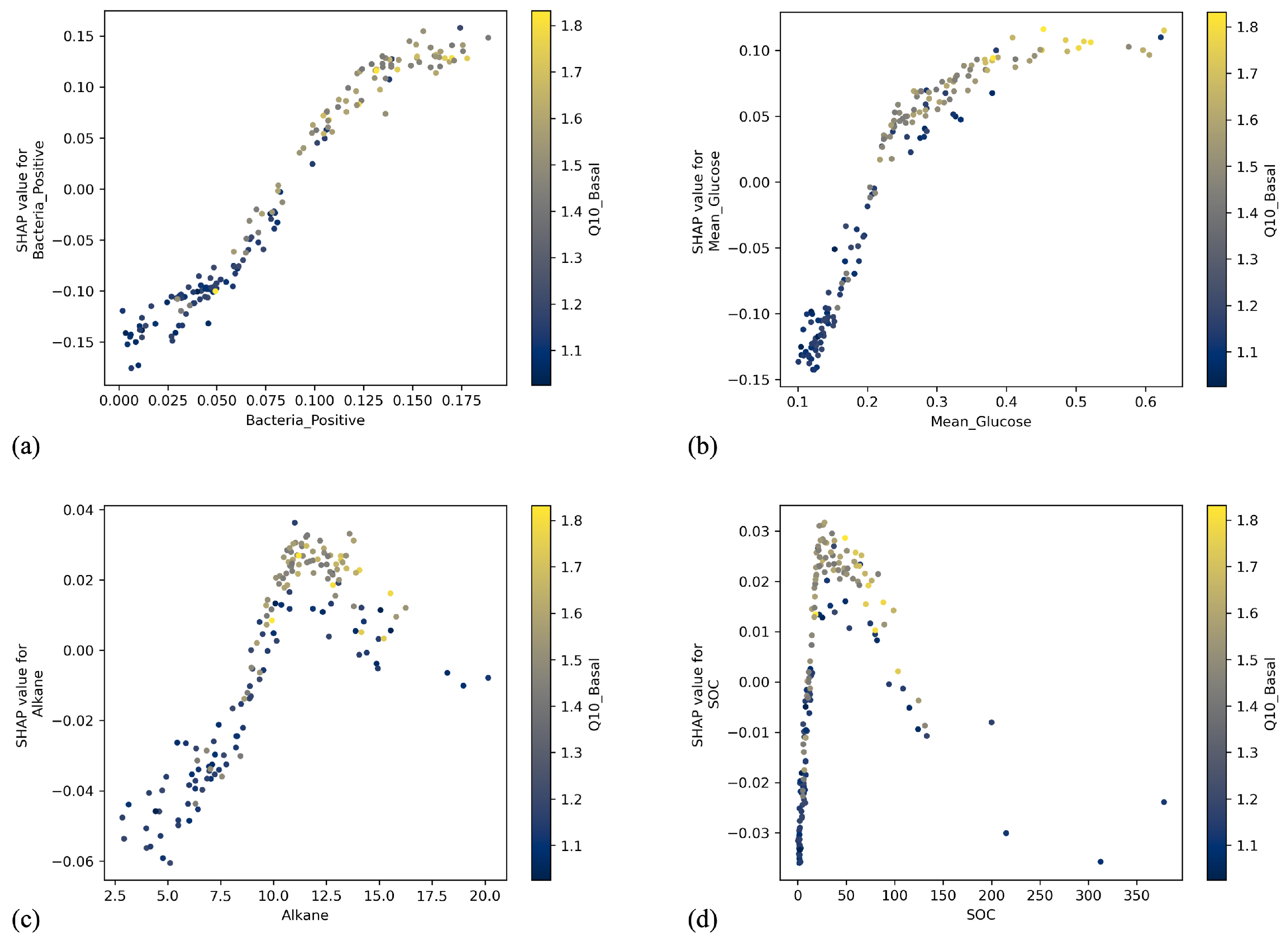
Furthermore, from Figure 3b, it emerges that out of the top 10 important features, eight are related to soil microbiome variables. The dependence plots shown in Figure 4 depict the marginal contributions of the four most important features according to Figure 3b. A dependence plot visualizes the relationship between a specific feature and its corresponding SHAP values, shedding light on how changes in the feature influence the model’s output. These plots represent the value of the variable on the x-axis, the SHAP value relative to this variable on the y-axis, and the color code referring to the Q10 value.
In particular, Figure 4a,b describe the dependence plot of two microbiome variables, respectively, “Bacteria_Positive” and “Mean_Glucose”; while Figure 4c,d describe the dependence plot of “Alkane” and “SOC”. Specifically, in the depicted dependence plots, an increase in the values of “Bacteria_Positive” and “Mean_Glucose” corresponds to a rise in the associated SHAP values. Consequently, elevated values of these variables play a significant role in the algorithm’s decision to classify an instance as high Q10.
An interesting behavior is observed in the dependence plots of “Alkane” and “SOC”, where an increase in the values of these features corresponds to a rise in the associated SHAP values until a certain threshold value. Beyond this threshold, the SHAP values begin to decrease. A further increase in Q10 values is observed for SOC up to a value between 20 and 50 g kg−1 dry soil; afterwards Q10 values decrease, notwithstanding the increase in SOC content. It is finally worth noting that with the global method obtained with embedded feature importance from the ML method, texture and soil pH were also selected among the 10 top important features.

4. Discussion

In our research, we have developed a robust artificial intelligence workflow capable of discerning the most influential factors among environmental, biochemical, and microbiome characteristics associated with high and low Q10 values within a cohort of over 300 soils. Recognizing the intricate interplay between the soil microbiome and food security is essential for developing sustainable agricultural practices that promote long-term food production. This workflow offers highly reliable predictions of Q10 outcomes for each individual soil sample, leveraging entirely data-driven classifiers. Understanding the composition and activity of the soil microbiome is, therefore, crucial for interpreting Q10 and its implications for soil biogeochemical processes. As can be seen in Table 2, the machine learning framework demonstrated strong predictive capabilities, underscoring the robustness of the models in forecasting the outcome. In contrast, the simpler Decision Tree model proved inadequate, showing significantly lower performance compared to the other models. Enhancing prediction accuracy necessitated the use of ensemble models, which delivered clearly higher results. Notably, the ExtraTrees classifier excelled, achieving the highest accuracy, area under the ROC curve, and area under the Precision-Recall Curve. These findings emphasize the importance of employing more complex models to capture the intricate relationships within the data and enhance predictive performance. In addition to decision tree ensembles, we evaluated the performance of Support Vector Machine (SVM), K-Nearest Neighbors (KNN), and Logistic Regression models. The results, summarized in Table 2, indicate that while these models provided reasonable accuracy, they did not achieve the same level of performance as the ensemble models. The ensemble methods, by leveraging multiple decision trees, captured more complex interactions and dependencies in the data, resulting in superior predictive accuracy. This comprehensive comparison underscores the importance of selecting appropriate models for high/low Q10 predictions and highlights the innovative framework we established for explainable machine learning.
Notably, the ML classifiers not only demonstrate high accuracy but also yield predictions that are readily interpretable. The XAI analysis reveals patterns aligning with established knowledge, particularly emphasizing the significance of soil microbiome in predicting soil Q10 [18,37,38,39,40]. The application of SHAP in this study provides a significant advantage over traditional embedded feature importance methods. Unlike global feature importance, which offers an overall ranking of features based on their average contribution across the entire dataset, SHAP values provide the specific feature contribution. This means SHAP can offer detailed interpretations and explanations for each individual instance, identifying which variables most significantly influenced the outcome and the direction of their effects for that specific instance. In this specific case, as shown in Figure 3b, using the SHAP value for the behavior of each individual soil sample, it is possible to understand how the variables influenced its classification as having high or low Q10. This granularity allows for targeted intervention strategies tailored to the specific characteristics of each soil.
The use of SHAP values highlights some significant relationships. Specifically, Figure 4 reveals that an increase in the values of the microbiome-related variables is positively correlated with an increase in the the temperature sensitivity of soil respiration prediction. This outcome was expected and supports the hypothesis of a direct relationship between these variables. Variables not associated with the microbiome exhibit more complex behavior. Initially, an increase in these variables is associated with a rise in the temperature sensitivity of soil respiration, indicating a positive effect up to a certain point. However, after reaching a critical threshold, further increases in these variables lead to a decrease in the Q10 value. This suggests a threshold effect, where non-microbiome-related variables positively contribute to Q10 prediction until a certain level is reached, beyond which their impact turns negative.
The behavior shown by the SHAP dependence plot is particularly relevant for soil organic carbon, due to its role as a main indicator of soil quality and health [41] and as a key regulator of temperature sensitivity to soil respiration [8]. A more in-depth assessment of the ranges and the threshold values involved in this response can greatly contribute to the understanding of ecosystem processes and to the prediction of soil carbon cycling responses to environmental changes. The feature importance analysis obtained from the ML method also highlighted the role of soil texture and pH in contributing to the model performance. Texture is a main physical, “use invariant”, soil property [41]. It strongly affects the soil structure and soil aggregates stability and regulates air–water capacity relationships, thus inducing changes in soil organic carbon dynamics and driving water holding capacity and soil moisture content [41,42,43]. This last factor is also known to significantly affect Q10 values [8]. The wide range of soil types encompassed in this study, with conditions ranging from coarse-textured soils, with clay and silt content of 0.49 g 100 g−1, to fine-textured soils, with clay and silt content of 88.2 g 100 g−1 [18], has certainly contributed to underlining the role of texture in driving soil respiration dynamics. This result also highlights the need to deepen the role of physical and hydraulic properties in future studies investigating the contribution of indicators such as soil aggregate size and stability, water retention properties, and hydraulic conductivity, in driving soil respiration and Q10 values at different spatial scales.
Furthermore, it is worth noting that this threshold effect seems to be observed in environmental variables rather than microbiome features, as observed from the dependence plots. Our findings highlight the significant role of the soil microbiome in shaping soil Q10 dynamics, underscoring its importance in soil biogeochemical processes and informing sustainable agricultural practices.

5. Conclusions

In this study, we employed an interpretable machine learning approach to investigate the influence of environmental, biochemical, and microbiome characteristics on soil microbial respiration sensitivity to warming (Q10). Our robust AI workflow demonstrated high predictive accuracy and interpretability, providing valuable insights into the factors driving soil Q10 variability.
Our findings highlight the significant role of the soil microbiome in shaping soil Q10 dynamics, underscoring its importance in soil biogeochemical processes and informing sustainable agricultural practices. Moreover, the exploration of extreme classes of Q10 may unearth biomarkers and facilitate a deeper understanding of the underlying dynamics, particularly elucidating key environmental, microbial, and biochemical factors that predominantly dictate soils with high or low Q10 values. Importantly, our predictive model operates at the level of individual soil samples, enabling practical application of the method to predict Q10 for specific soil samples in real-world scenarios.
We implemented an Explainable Artificial Intelligence (XAI) strategy to understand how our classification model predicts outcomes, focusing on feature importance using SHapley Additive exPlanations (SHAP). This approach allows us to interpret the influence of each variable on predictions for individual soil samples, providing detailed insights into soil respiration sensitivity to warming. The SHAP results highlighted the significant importance of variables such as bacteria positive, SOC (soil organic carbon), alkane, and mean glucose. Our work aims to elucidate the relationships between the Q10 value and various soil, environmental, and land use variables, particularly microbiome composition, addressing the global need to mitigate greenhouse gas emissions. This comprehensive understanding is crucial for making informed decisions to protect ecosystems and adapt to ongoing climate change.
Moving forward, our research emphasizes the importance of leveraging AI-driven approaches to better understand complex soil–ecosystem interactions and inform sustainable agricultural practices. By elucidating the factors influencing soil Q10, we can develop targeted strategies to enhance soil health, optimize crop production, and ensure agricultural sustainability in the face of environmental challenges.

Author Contributions

Conceptualization, M.M., P.N. and S.T.; methodology, M.M., P.N. and S.T.; software, M.M. and P.N.; validation, M.M., P.N. and S.T.; formal analysis, M.M. and P.N.; investigation, M.M. and P.N.; resources, M.M. and P.N.; data curation, M.M. and P.N.; writing—original draft preparation, M.M., P.N. and S.T.; writing—review and editing, all authors; visualization, M.M., P.N. and S.T.; supervision, S.T.; project administration, S.T.; funding acquisition, S.T. All authors have read and agreed to the published version of the manuscript.

Funding

The METROFOOD-IT project has received funding from the European Union—NextGeneration-EU, PNRR—Mission 4 “Education and Research” Component 2: from research to business, Investment 3.1: Fund for the realization of an integrated system of research and innovation infrastructures—IR0000033 (D.M. Prot. n.120 del 21 June 2022); TEBAKA (TErritorial BAsic Knowledge Acquisition project “Avviso MIUR n.1735 del 13 July 2017”; The National Recovery and Resilience Plan (NRRP), Mission 4 Component 2 Investment 1.4—Call for tender No. 3138 of 16 December 2021 of Italian Ministry of University and Research funded by the European Union—NextGenerationEU. Award Number: Project code: CN00000022, Concession Decree No. 1031 of 17 February 2022 adopted by the Italian Ministry of University and Research, CUP H93C22000440007, Project title: “National Research Centre for Agricultural Technologies (Agritech)”.

Data Availability Statement

All data utilized in the analysis are publicly available and have been downloaded from the repository on Figshare at the following DOI: https://doi.org/10.6084/m9.figshare.20776243.v1 (accessed on 1 July 2024) [18].

Acknowledgments

The authors are grateful for the resources made available by ReCaS, a project funded by the MIUR (Italian Ministry for Education, University and Research) in the “PON Ricerca e Competitività 2007–2013-Azione I-Interventi di rafforzamento strutturale” PONa3_00052, Avviso 254/Ric, University of Bari.

Conflicts of Interest

The authors declare no conflict of interest.

References

  1. Allen, D.E.; Singh, B.P.; Dalal, R.C. Soil health indicators under climate change: A review of current knowledge. In Soil Health and Climate Change; Springer: Berlin/Heidelberg, Germany, 2011; pp. 25–45. [Google Scholar]
  2. Lal, R. Soil health and climate change: An overview. In Soil Health and Climate Change; Springer: Berlin/Heidelberg, Germany, 2011; pp. 3–24. [Google Scholar]
  3. Patil, A.; Lamnganbi, M. Impact of climate change on soil health: A review. Int. J. Chem. Stud 2018, 6, 2399–2404. [Google Scholar]
  4. Haaf, D.; Six, J.; Doetterl, S. Global patterns of geo-ecological controls on the response of soil respiration to warming. Nat. Clim. Change 2021, 11, 623–627. [Google Scholar] [CrossRef]
  5. Reeve, J.R.; Hoagland, L.A.; Villalba, J.J.; Carr, P.M.; Atucha, A.; Cambardella, C.; Davis, D.R.; Delate, K. Organic farming, soil health, and food quality: Considering possible links. Adv. Agron. 2016, 137, 319–367. [Google Scholar]
  6. Crowther, T.W.; Van den Hoogen, J.; Wan, J.; Mayes, M.A.; Keiser, A.; Mo, L.; Averill, C.; Maynard, D.S. The global soil community and its influence on biogeochemistry. Science 2019, 365, eaav0550. [Google Scholar] [CrossRef] [PubMed]
  7. Mahecha, M.D.; Reichstein, M.; Carvalhais, N.; Lasslop, G.; Lange, H.; Seneviratne, S.I.; Vargas, R.; Ammann, C.; Arain, M.A.; Cescatti, A.; et al. Global convergence in the temperature sensitivity of respiration at ecosystem level. Science 2010, 329, 838–840. [Google Scholar] [CrossRef] [PubMed]
  8. Meyer, N.; Welp, G.; Amelung, W. The temperature sensitivity (Q10) of soil respiration: Controlling factors and spatial prediction at regional scale based on environmental soil classes. Glob. Biogeochem. Cycles 2018, 32, 306–323. [Google Scholar] [CrossRef]
  9. Rolnick, D.; Donti, P.L.; Kaack, L.H.; Kochanski, K.; Lacoste, A.; Sankaran, K.; Ross, A.S.; Milojevic-Dupont, N.; Jaques, N.; Waldman-Brown, A.; et al. Tackling climate change with machine learning. ACM Comput. Surv. (CSUR) 2022, 55, 1–96. [Google Scholar] [CrossRef]
  10. Huntingford, C.; Jeffers, E.S.; Bonsall, M.B.; Christensen, H.M.; Lees, T.; Yang, H. Machine learning and artificial intelligence to aid climate change research and preparedness. Environ. Res. Lett. 2019, 14, 124007. [Google Scholar] [CrossRef]
  11. Wilhelm, R.C.; van Es, H.M.; Buckley, D.H.. Predicting measures of soil health using the microbiome and supervised machine learning. Soil Biol. Biochem. 2022, 164, 108472. [Google Scholar]
  12. Papoutsoglou, G.; Tarazona, S.; Lopes, M.B.; Klammsteiner, T.; Ibrahimi, E.; Eckenberger, J.; Novielli, P.; Tonda, A.; Simeon, A.; Shigdel, R.; et al. Machine learning approaches in microbiome research: Challenges and best practices. Front. Microbiol. 2023, 14, 1261889. [Google Scholar] [CrossRef]
  13. Di Gilio, A.; Catino, A.; Lombardi, A.; Palmisani, J.; Facchini, L.; Mongelli, T.; Varesano, N.; Bellotti, R.; Galetta, D.; de Gennaro, G.; et al. Breath analysis for early detection of malignant pleural mesothelioma: Volatile organic compounds (VOCs) determination and possible biochemical pathways. Cancers 2020, 12, 1262. [Google Scholar] [CrossRef] [PubMed]
  14. Cascio, D.; Taormina, V.; Cipolla, M.; Bruno, S.; Fauci, F.; Raso, G. A multi-process system for HEp-2 cells classification based on SVM. Pattern Recognit. Lett. 2016, 82, 56–63. [Google Scholar] [CrossRef]
  15. Biecek, P.; Burzykowski, T. Explanatory Model Analysis: Explore, Explain, and Examine Predictive Models; Chapman and Hall/CRC: Boca Raton, FL, USA, 2021. [Google Scholar]
  16. Ghalebikesabi, S.; Ter-Minassian, L.; DiazOrdaz, K.; Holmes, C.C. On locality of local explanation models. Adv. Neural Inf. Process. Syst. 2021, 34, 18395–18407. [Google Scholar]
  17. Li, Z. Extracting spatial effects from machine learning model using local interpretation method: An example of SHAP and XGBoost. Comput. Environ. Urban Syst. 2022, 96, 101845. [Google Scholar] [CrossRef]
  18. Sáez-Sandino, T.; García-Palacios, P.; Maestre, F.T.; Plaza, C.; Guirado, E.; Singh, B.K.; Wang, J.; Cano-Díaz, C.; Eisenhauer, N.; Gallardo, A.; et al. The soil microbiome governs the response of microbial respiration to warming across the globe. Nat. Clim. Change 2023, 13, 1382–1387. [Google Scholar] [CrossRef]
  19. Nottingham, A.T.; Whitaker, J.; Turner, B.L.; Salinas, N.; Zimmermann, M.; Malhi, Y.; Meir, P. Climate warming and soil carbon in tropical forests: Insights from an elevation gradient in the Peruvian Andes. Bioscience 2015, 65, 906–921. [Google Scholar] [CrossRef] [PubMed]
  20. Winkler, J.P.; Cherry, R.S.; Schlesinger, W.H. The Q10 relationship of microbial respiration in a temperate forest soil. Soil Biol. Biochem. 1996, 28, 1067–1072. [Google Scholar] [CrossRef]
  21. Steyerberg, E.W.; Steyerberg, E.W. Coding of categorical and continuous predictors. In Clinical Prediction Models: A Practical Approach to Development, Validation, and Updating; Springer: Cham, Switzerland, 2019; pp. 175–190. [Google Scholar]
  22. Ibrahimi, E.; Lopes, M.B.; Dhamo, X.; Simeon, A.; Shigdel, R.; Hron, K.; Stres, B.; D’Elia, D.; Berland, M.; Marcos-Zambrano, L.J. Overview of data preprocessing for machine learning applications in human microbiome research. Front. Microbiol. 2023, 14, 1250909. [Google Scholar] [CrossRef] [PubMed]
  23. Ahsan, M.M.; Mahmud, M.P.; Saha, P.K.; Gupta, K.D.; Siddique, Z. Effect of data scaling methods on machine learning algorithms and model performance. Technologies 2021, 9, 52. [Google Scholar] [CrossRef]
  24. Cortes, C.; Vapnik, V. Support-vector networks. Mach. Learn. 1995, 20, 273–297. [Google Scholar] [CrossRef]
  25. Guo, G.; Wang, H.; Bell, D.; Bi, Y.; Greer, K. KNN model-based approach in classification. In On The Move to Meaningful Internet Systems 2003: CoopIS, DOA, and ODBASE. OTM; Lecture Notes in Computer Science; Meersman, R., Tari, Z., Schmidt, D.C., Eds.; Springer: Berlin/Heidelberg, Germany, 2003; Volume 2888, pp. 986–996. [Google Scholar]
  26. LaValley, M.P. Logistic regression. Circulation 2008, 117, 2395–2399. [Google Scholar] [CrossRef] [PubMed]
  27. Swain, P.H.; Hauska, H. The decision tree classifier: Design and potential. IEEE Trans. Geosci. Electron. 1977, 15, 142–147. [Google Scholar] [CrossRef]
  28. Breiman, L. Random forests. Mach. Learn. 2001, 45, 5–32. [Google Scholar] [CrossRef]
  29. Geurts, P.; Ernst, D.; Wehenkel, L. Extremely randomized trees. Mach. Learn. 2006, 63, 3–42. [Google Scholar] [CrossRef]
  30. Chen, T.; Guestrin, C. Xgboost: A scalable tree boosting system. In Proceedings of the 22nd ACM sigkdd International Conference on Knowledge Discovery and Data Mining, San Francisco, CA, USA, 13–17 August 2016; pp. 785–794. [Google Scholar]
  31. Aydın, Y.; Işıkdağ, Ü.; Bekdaş, G.; Nigdeli, S.M.; Geem, Z.W. Use of machine learning techniques in soil classification. Sustainability 2023, 15, 2374. [Google Scholar] [CrossRef]
  32. Ferrer, L. Analysis and comparison of classification metrics. arXiv 2022, arXiv:2209.05355. [Google Scholar]
  33. Ozenne, B.; Subtil, F.; Maucort-Boulch, D. The precision–recall curve overcame the optimism of the receiver operating characteristic curve in rare diseases. J. Clin. Epidemiol. 2015, 68, 855–859. [Google Scholar] [CrossRef]
  34. Wen, P.; Xu, Q.; Yang, Z.; He, Y.; Huang, Q. Algorithm-Dependent Generalization of AUPRC Optimization: Theory and Algorithm. IEEE Trans. Pattern Anal. Mach. Intell. 2024, 46, 5062–5079. [Google Scholar] [CrossRef]
  35. Novielli, P.; Romano, D.; Magarelli, M.; Bitonto, P.D.; Diacono, D.; Chiatante, A.; Lopalco, G.; Sabella, D.; Venerito, V.; Filannino, P.; et al. Explainable Artificial Intelligence for Microbiome Data Analysis in Colorectal Cancer Biomarker Identification. Front. Microbiol. 2024, 15, 1348974. [Google Scholar] [CrossRef]
  36. Lundberg, S.M.; Lee, S.I. A unified approach to interpreting model predictions. Adv. Neural Inf. Process. Syst. 2017, 30. [Google Scholar] [CrossRef]
  37. Ali, R.S.; Poll, C.; Kandeler, E. Dynamics of soil respiration and microbial communities: Interactive controls of temperature and substrate quality. Soil Biol. Biochem. 2018, 127, 60–70. [Google Scholar] [CrossRef]
  38. Jansson, J.K.; Hofmockel, K.S. Soil microbiomes and climate change. Nat. Rev. Microbiol. 2020, 18, 35–46. [Google Scholar] [CrossRef] [PubMed]
  39. Yang, S.; Wu, H.; Wang, Z.; Semenov, M.V.; Ye, J.; Yin, L.; Wang, X.; Kravchenko, I.; Semenov, V.; Kuzyakov, Y.; et al. Linkages between the temperature sensitivity of soil respiration and microbial life strategy are dependent on sampling season. Soil Biol. Biochem. 2022, 172, 108758. [Google Scholar] [CrossRef]
  40. Tong, D.; Li, Z.; Xiao, H.; Nie, X.; Liu, C.; Zhou, M. How do soil microbes exert impact on soil respiration and its temperature sensitivity? Environ. Microbiol. 2021, 23, 3048–3058. [Google Scholar] [CrossRef] [PubMed]
  41. Reynolds, W.; Drury, C.; Tan, C.; Fox, C.; Yang, X. Use of indicators and pore volume-function characteristics to quantify soil physical quality. Geoderma 2009, 152, 252–263. [Google Scholar] [CrossRef]
  42. Popolizio, S.; Stellacci, A.M.; Giglio, L.; Barca, E.; Spagnuolo, M.; Castellini, M. Seasonal and soil use dependent variability of physical and hydraulic properties: An assessment under minimum tillage and no-tillage in a long-term experiment in southern Italy. Agronomy 2022, 12, 3142. [Google Scholar] [CrossRef]
  43. Reynolds, W.; Bowman, B.; Drury, C.; Tan, C.; Lu, X. Indicators of good soil physical quality: Density and storage parameters. Geoderma 2002, 110, 131–146. [Google Scholar] [CrossRef]
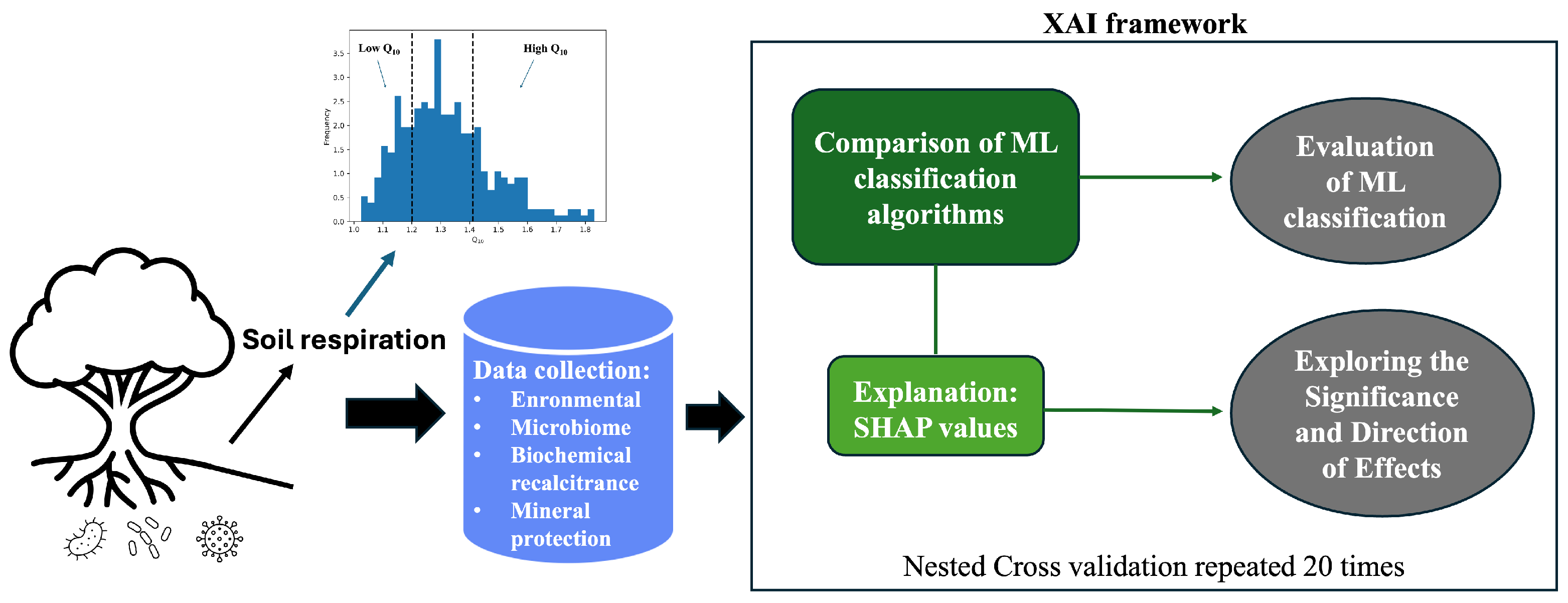
Figure 1. Analysis workflow for identification of factors that most influence soil with high Q10 and low Q10.
Make 06 00075 g001
Figure 2. Average Receiver Operating Characteristic (ROC) curve (a,b) Precision-Recall Curve (PRC) obtained through 10-fold cross-validation repeated 20 times.
Make 06 00075 g002
Figure 3. Global feature importance obtained with embedded feature importance from the machine learning model (a) and feature importance calculated with SHAP (b). Feature importance boxplots (a) describe the distribution of feature importance and identify any features that have significant relevance in the model. The “box” represents the interquartile range (IQR) of the feature importance, with the median line indicating the central value. The “whiskers” (lines extending from the box) show the variation beyond the IQR, while points outside the whisker range can be considered outliers. The SHAP (SHapley Additive exPlanations) summary plot (b) provides an overview of the importance of features in contributing to model predictions. In this type of plot, each point represents a data instance, and the horizontal position of the point indicates how much the effect of a specific feature contributes to the change in prediction compared to the model’s average prediction. The color of the point represents the value of the feature, with darker colors indicating higher values.
Make 06 00075 g003
Figure 4. Dependence plots illustrating the marginal contributions of the four most important features according to SHAP values. (a,b) depict the dependence plots of two microbiome variables, while (c,d) represent the dependence plots of the other two variables.
Make 06 00075 g004
Table 1. Description of the input variables used in the analysis.
VariableDescriptionUnits
Longitude_cLongitudeDecimal degree
ForestPresence of forestunitless
MAP_wc2Mean annual precipitationmm
MAT_wc2Mean annual temperature°C
Plant_richnessNumber of speciesunitless
Plant_cover_v3Proportion of the plant that extends into the soilunitless
Soil_pHpH of soilunitless
Soil_salinityElectrical conductivitydS m−1
Fine_texturePercentage of clay and silt in the soilg 100 g−1 dry soil
Soil_PSoil total phosphorusmg P kg −1 dry soil
Soil_CNRatio between total organic carbon and total Nunitless
SOCSoil organic carbong C kg−1 soil
MAOC/POC_RatioRatio between proportion of mineral-associated organic C and proportion of particulate organic Cunitless
AromaticPercentage of aromaticunitless
AlkanesPercentage of alkaneunitless
PolysaccharidePercentage of polysaccharideunitless
AmidePercentage of amideunitless
Mean_GlucoseGlucose-induced soil respiration μ g CO2-C g−1 soil h−1
Richness_bacteriaRichness of bacteriaNumber of zOTUs
Richness_fungiRichness of fungiNumber of zOTUs
Richness_protistRichness of protistNumber of zOTUs
Bacteria_NegativeStandardized proportion of bacteria taxa negatively associated with Q10unitless
Fungi_NegativeStandardized proportion of fungi taxa negatively associated with Q10unitless
Protists_NegativeStandardized proportion of protist taxa negatively associated with Q10unitless
Bacteria_PositiveStandardized proportion of bacteria taxa positively associated with Q10unitless
Fungi_PositiveStandardized proportion of fungi taxa positively associated with Q10unitless
Protists_PositiveStandardized proportion of protist taxa positively associated with Q10unitless
Table 2. Average performance of machine learning classifiers obtained through 10-fold cross-validation repeated 20 times.
ML ClassifierAccuracyAUROCAUPRC
Extra Trees0.923 ± 0.0090.964 ± 0.0040.963 ± 0.006
XGBoost0.899 ± 0.0080.932 ± 0.0060.899 ± 0.012
Random Forest0.920 ± 0.0070.951 ± 0.0050.939 ± 0.013
Decision Tree0.838 ± 0.0220.862 ± 0.0270.861 ± 0.031
SVM0.901 ± 0.0130.946 ± 0.0100.930 ± 0.029
KNN0.883 ± 0.0160.947 ± 0.0070.951 ± 0.006
Logistic Regression0.901 ± 0.0100.941 ± 0.0100.923 ± 0.029
Disclaimer/Publisher’s Note: The statements, opinions and data contained in all publications are solely those of the individual author(s) and contributor(s) and not of MDPI and/or the editor(s). MDPI and/or the editor(s) disclaim responsibility for any injury to people or property resulting from any ideas, methods, instructions or products referred to in the content.