2.1. Aboveground Biomass Database
Funded by the United States Agency for International Development (USAID) and the Global Livestock Collaborative Research Support Program (GL-CRSP), a network of monitoring sites was installed in Kenya beginning in 1999 onward as an integral component of the broader Livestock Early Warning System (LEWS) for East Africa [
35]. The network in Kenya was expanded beginning in 2015 as part of a collaboration among the Food and Agriculture Organization (FAO), Texas A&M AgriLife Research (TAMU), and the Kenya National Drought Management Authority (KNDMA), and became part of the Predictive Livestock Early Warning System in East Africa [
4,
36]. The main objectives of the monitoring network were to provide near real-time assessments of aboveground biomass that could be grazed by livestock and to enable the near-term (30–90 days) and mid-term (90–180 day) forecasting of aboveground biomass to aid pastoralists and other stakeholders in assessing risk. At monitoring sites, field data were collected to parameterize and calibrate the Phytomass Growth Model (PHYGROW) [
4] and generate near real-time aboveground biomass time series at the monitoring sites throughout Kenya [
4,
35,
37]. While the present study is distinct from the PHYGROW model and the Predictive Livestock Early Warning System, it leverages the model’s generated time series data to conduct near-term biomass forecasts. The dataset used in this study is available at:
https://github.com/noayarae/multi_output_time_series_forecasting_methods_with_CNN (accessed on 21 May 2024).
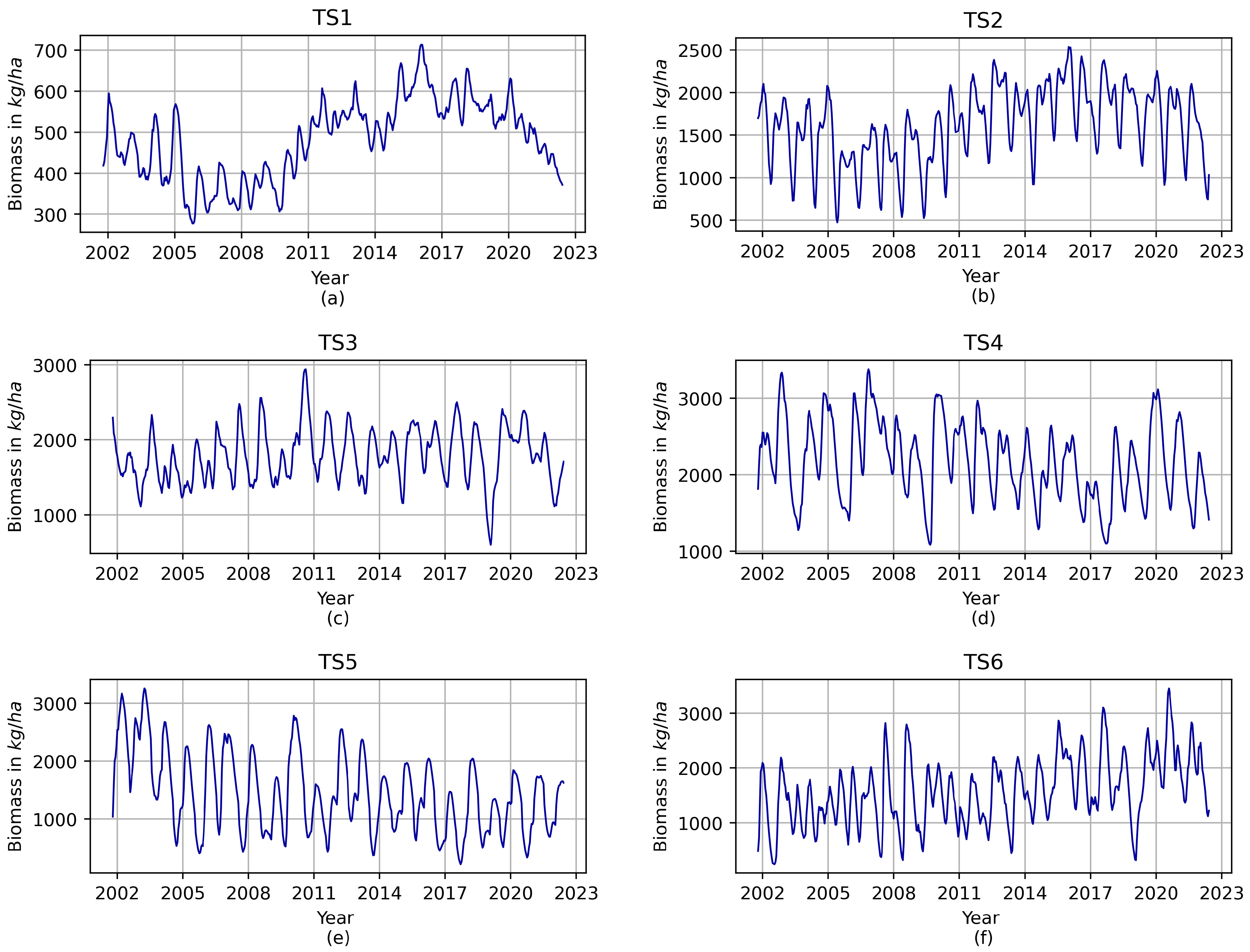
For this study, we selected six time series that represent aboveground biomass, comprising the model outputs at 15-day intervals from 14 January 2002 to 31 August 2022. As a result, each time series comprises a total of 496 aboveground biomass estimates in kg/ha. To ensure data quality, these chosen time series underwent meticulous visual examination for any irregularities or unusual patterns, whether isolated events or chronological sequences.
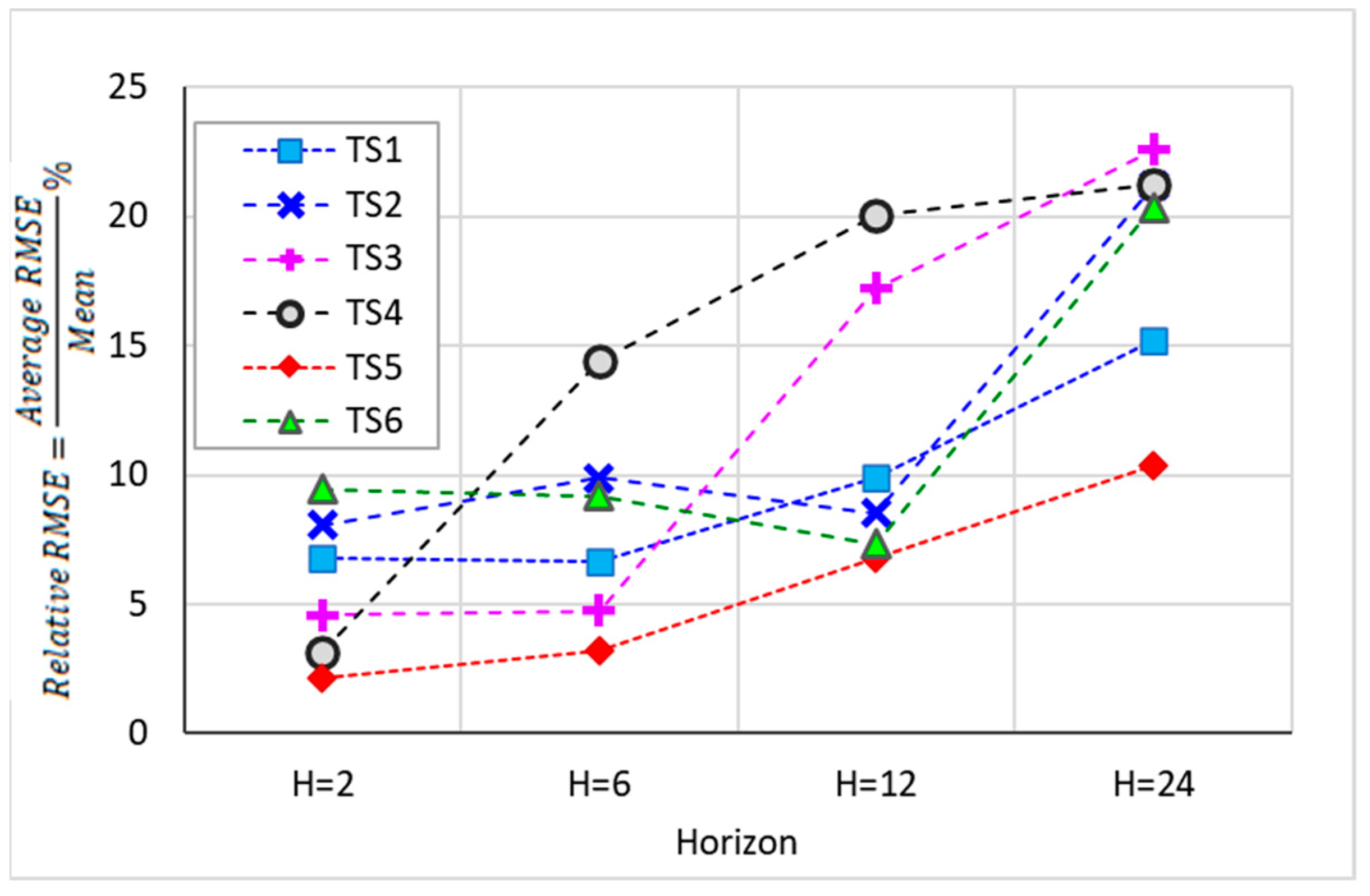
Figure 1 illustrates the assessed time series of aboveground vegetation biomass for the selected monitoring sites. It is noteworthy that the selected time series effectively capture a wide spectrum of regional aboveground biomass production rates within the study area, ranging from an average low of 104.5 kg/ha to an average high of 3171.5 kg/ha.
2.2. Data Preprocessing
The time series
underwent preprocessing aimed at enhancing the efficiency of the model training process and mitigating potential complications, such as vanishing gradients, which could otherwise speed up model convergence. In this regard, normalization played a pivotal role in minimizing the model’s susceptibility to variations in the scale of input features, ultimately bolstering its capacity for generalization. The normalization procedure was executed by rescaling the data within the range from 0 to 1 using the following equation:
where
is the time series value,
is the normalized value,
is the highest value of the time series, and
is the lowest value of the time series. Applying this normalization procedure ensured consistent data scaling, improving training, convergence, and model generalization—all crucial for research success.
In transforming the time series data into a supervised dataset, the time series was partitioned into two subseries. The first 472 data points were utilized for training the model, while the remaining 24 data points (one year of data) were designated for model testing. The training time subseries was then structured into a supervised database with predictor and response values to facilitate the application of the CNN algorithm. This structuring process primarily involved extracting short subsequences from the training series, with each subsequence containing one segment designated as predictor values (
w) and another segment designated as response values (
k). The length of the predictor segments (representing independent variables) was consistently set at 24 values, while the length of the response segments (representing dependent variables) varied between 1 and 24, depending on the multi-output case under consideration. For instance, if we considered the scenario of multi-output forecasting where three values were predicted simultaneously (
k = 3), the subsequences would consist of 27 data points
, with the first 24 designated as predictors and the remaining 3 as response values. Subsequently, the process repeated, shifting forward one time step within the training time subseries, until the last data point of the training subseries (
) was reached/included (
Figure 2). Thus, the total number of subsequences obtained was determined as
.
2.3. Methods for Multi-Output Time Series Forecasting
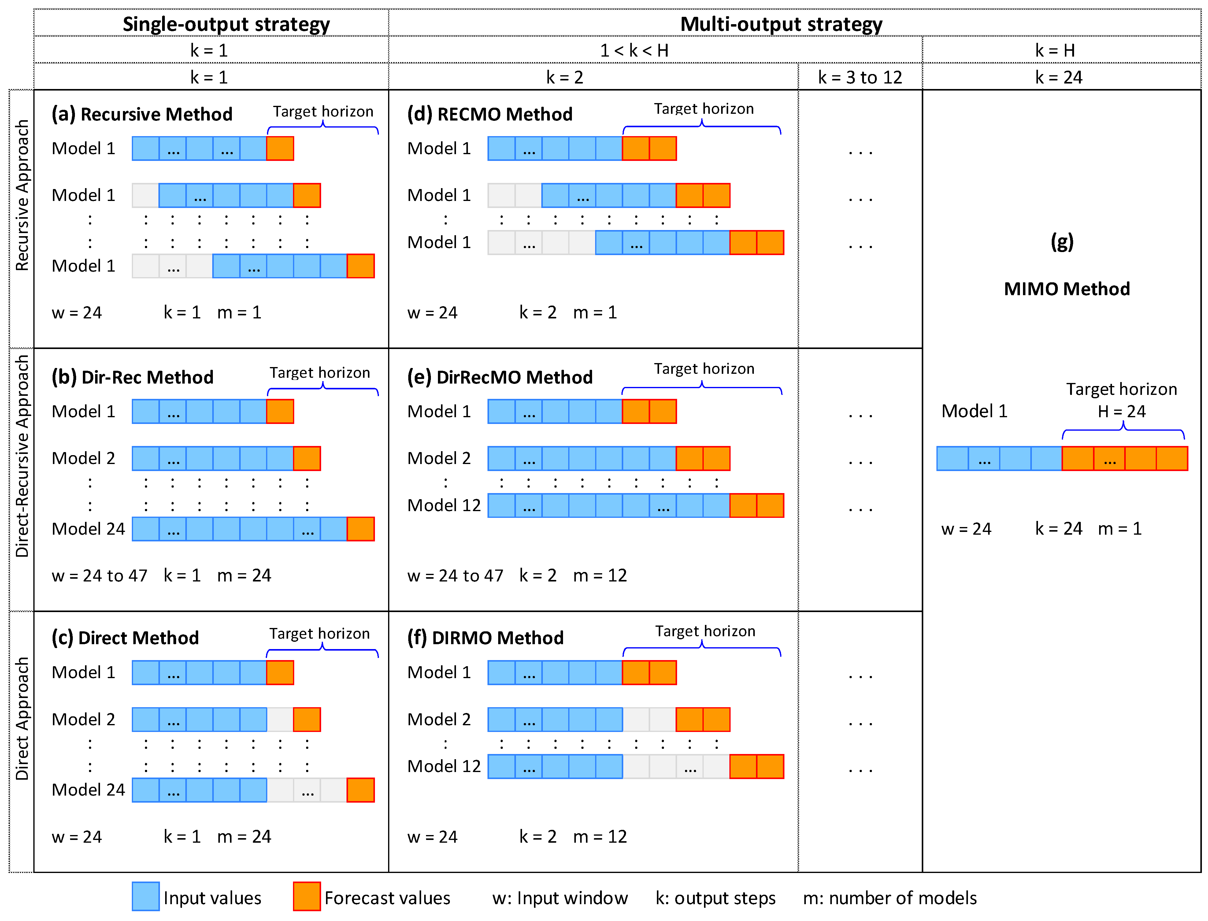
Existing methodologies for time series forecasting using AI algorithms can be categorized into single-step forecasting methods and multi-step forecasting methods. For target horizons beyond a single step, single-step methods typically involve repeated predictions until the target horizon is attained, whereas multi-step methods directly forecast either all or a portion of the target horizon values. The first category includes the recursive, direct, and DirRec methods, and the second category includes the MIMO and DIRMO approaches. Additionally, our work introduces two novel methods in the latter category: RECMO and DirRecMO. Each of these existing and novel methods are described in greater detail below.
Figure 3 provides an overview of each of these forecasting methods specifically for a target horizon of 24 (H = 24).
The recursive, also called iterative, approach entails step-by-step forecasting. This method typically advances one time step at a time until the target forecast horizon (
) is attained, thus requiring a total of
iterations (Equation (2)) [
20]. In each iteration, the previously forecasted value is included in the input for the next prediction, while the most remote past value is excluded. This ensures that the input window size (
) remains constant across all iterations; thus, this technique is often characterized as the “sliding window” approach (
Figure 3a). Using a single forecast model in all iterations makes this method fast and practical. However, any errors in a prediction carry forward and accumulate in subsequent forecasts.
where
is the forecast value and
represents the single forecast model.
The direct method predicts each time point within the horizon independently, using a different AI model specifically fitted for each point value [
29]. As a result, the number of prediction models equals the length of the target horizon (
) (Equation (3)). Because there is no recursive feeding of predicted values into the input for subsequent predictions, this technique prevents error accumulation over the predicted time points. This approach maintains a constant window size and input values for all predictions (
Figure 3c).
where
with (
) represents the distinct prediction models.
The direct-recursive (DirRec) method represents a hybrid of the direct (Dir) and recursive (Rec) methods. Like the direct method, the DirRec method applies a distinct model at each time point within the forecast horizon [
21] and the total number of models matches the length of the target horizon. As in the recursive (iterative) method, these models incorporate previous predictions. Because each prediction is included in the input for the subsequent forecast without excluding any past values, the input window length expands with each iteration; thus, this method is known as the “expanding window” approach (
Figure 3b).
The Multiple-Input Multiple-Output (MIMO) method is a forecasting approach where the model predicts multiple output values simultaneously. This entails configuring the model’s output layer to align with the target forecast horizon, facilitating the concurrent prediction of multiple data points. Particularly valuable for capturing dependencies in time series forecasting, this method overcomes the limitations of single-step models that assume stochastic independence, mitigating bias in longer horizons [
23]. Due to its multi-output nature, the method requires only one model for a given target horizon, thereby reducing the number of models and iterations as compared to single-step models (
Figure 3g). All future values within the target horizon are predicted by:
The DIRMO method integrates aspects of the DIRect and the miMO strategies by decomposing the forecast horizon into numerous multi-outcome segments [
23,
38]. This strategy balances the flexibility of multiple models with the stochastic dependencies within each multi-output model. This is equivalent to extending the direct model to forecast several values at the same time (e.g., 2, 3, or more consecutive steps ahead), effectively decreasing the requirement for multiple models (
Figure 3f). The DIRMO method considers the parameter ‘
k’ to define the number of steps ahead predicted at each pace (multi-output), resulting in a total of
models, where
and 1 <
k <
H. At range edges, when
k = 1, it becomes the direct method; when k = H, it becomes MIMO. The multi-output DIRMO forecasting method is expressed as:
where
is the iteration number
and
is computed by
. As an illustration, when
,
, and
, we find that
, resulting in
being
and
being
. Therefore, we will utilize three models for multi-output forecasting, where each model simultaneously predicts eight values to achieve the total length of the target horizon.
This method integrates the concepts of the RECursive and miMO strategies, breaking down the forecast horizon into multi-output segments and processing them recursively. Similar to DIRMO, the RECMO method incorporates the parameter
to specify the number of steps ahead predicted in each iteration. During each iteration, the forecast model predicts the next k-steps (where
). These predicted k-steps become part of the input window for subsequent iterations. By including the previously predicted k values and excluding the most remote k value from the input window, the window size remains constant across all iterations but shifts in k time steps, resembling the “sliding window” of the recursive method (
Figure 3d). With this modification, the number of iterations (
n) is scaled down to the quotient between the target horizon and the k-steps predicted ahead at each time (
). At
k’s limits, it is recursive for
k = 1 and MIMO for
k =
H. In such instances, Equation (2) can be extended to Equation (7):
where
is the iteration number
and
is computed by
. As an illustration, when
,
, and
, we find that
, resulting in
being
and
being
. Therefore, the equations for multi-step (eight-step) iterative forecasting are provided by the following three expressions:
The DirRecMO method integrates the Direct, Recursive, and MIMO strategies, essentially extending the DirRec method by predicting multi-output values (
k) in each iteration (where
). Like the recursive method, it uses the predicted multi-output values as inputs for subsequent predictions until the target horizon is reached; however, the input window does not slide, but instead expands with each iteration, as in the DirRec method (
Figure 3e). Like the Direct method, AI models are distinct at each iteration. With k output values predicted per iteration (
), the number of models is
. At
k’s limits, it becomes the DirRec method for
k = 1 and the MIMO method for
k =
H. Thus, all future values within the target horizon are predicted by:
For example, for
,
, and
, we have
,
and
, and the forecasting equations simplify to:
2.4. Modeling, Prediction, and Experimental Baselines
The main settings included the AI model, input window size (
w), prediction horizon (
H), multi-output size (
k), number of models (
m), and replications. The forecasting methods were assessed using the AI CNN model, known for its performance in reliably predicting biomass time series [
34]. To mitigate randomness, 20 replications were conducted for each combination of horizon and k value, ensuring robust outcomes. The input window size for the forecasting methods with no expanding window, (i.e., Recursive, Direct, MIMO, RECMO, and DIRMO) was fixed at 24, in accordance with prior studies suggesting an input length akin to the horizon length. In methods with an expanding window (i.e., DirRec and DirRecMO), the input size varied from 24 to 47 based on the multi-output size, horizon length, and method used. The target horizons (
H) evaluated were 2, 6, 12, and 24 data values ahead, corresponding to 1, 3, 6, and 12 months, respectively. These horizons were strategically selected to align with the practical needs of early warning system stakeholders. For instance, planners frequently demand forecasts of six and twelve months (long-term) to facilitate comprehensive planning. Pastoralists and ranchers, on the other hand, are interested in one-month forecasts (short-term) and three-month forecasts (medium-term) to make informed decisions on critical issues like forage scarcity related to drought duration and intensity. The multi-output sizes were set to the maximum allowable number based on the target horizon. For instance, when considering a horizon of 24 values, we assessed eight multi-output sizes (
), which are all divisors of 24. For one-month horizons, only two multi-output sizes were assessed (
. The number of models (
m) varied based on the forecasting method, horizon, and multi-output size. For instance, for a horizon of 12 and
k = 4, the recursive method uses one model, while DIRMO requires three.
Table 1 summarizes the methods’ key parameters and settings.
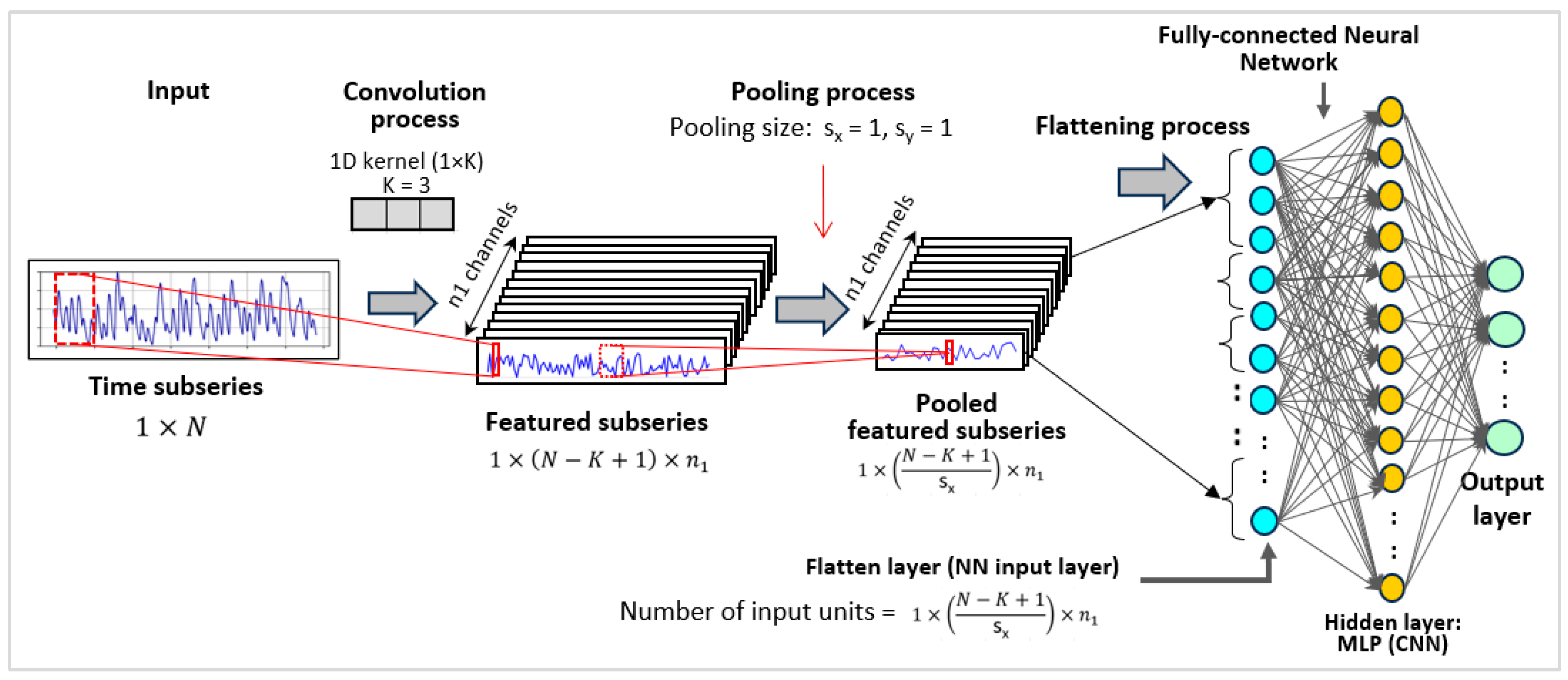
The CNN algorithm, designed for complex data processing, has proven effective in simulating time series data [
39]. CNNs integrate advanced data preprocessing techniques, including convolution layers and pooling layers, preceding the fully connected layers. These networks excel in capturing hierarchical patterns and spatial correlations within data, increasing their proficiency in image recognition and feature extraction and enabling them to capture temporal patterns in sequential data [
40].
Figure 4 outlines the structure of the CNN algorithm, beginning with an input layer subjected to a convolution process [
34]. The input time subseries corresponds to the input window of each subsequence obtained during data preprocessing (
Section 2.2). Each subsequence is represented as a subseries of length
. This subseries is convoluted using a 1D kernel of size
(
), resulting in a new subseries of length
. Thus, with
kernels applied,
subseries are obtained, each of length
. To retain information in these short subseries, the pooling size is set to 1 (
), so the number and length of the subseries remain
and (
), respectively. Each subseries is then flattened to form the flatten layer (NN input layer), with the number of nodes computed as
, followed by a set of fully interconnected nodes in hidden layers [
41]. The flattened and hidden layers generate the output layer. The output layer varies for single-output tasks, and it has one node; for multi-output tasks, it matches the multi-output size
, as detailed in
Table 1. The manual fine-tuning of hyperparameters in the CNN model aimed to minimize prediction errors, with the specific values detailed in
Table 2.
2.5. Model Performance Evaluation
Model performance was evaluated using several metrics. First, we employed the Root Mean Square Error (RMSE), which is calculated as:
In this equation, represents the observed time series value at time i, is the estimated/forecast time series value at time i, and is the number of data points. RMSE values can range from zero to infinity, with zero indicating a perfect model with no prediction error.
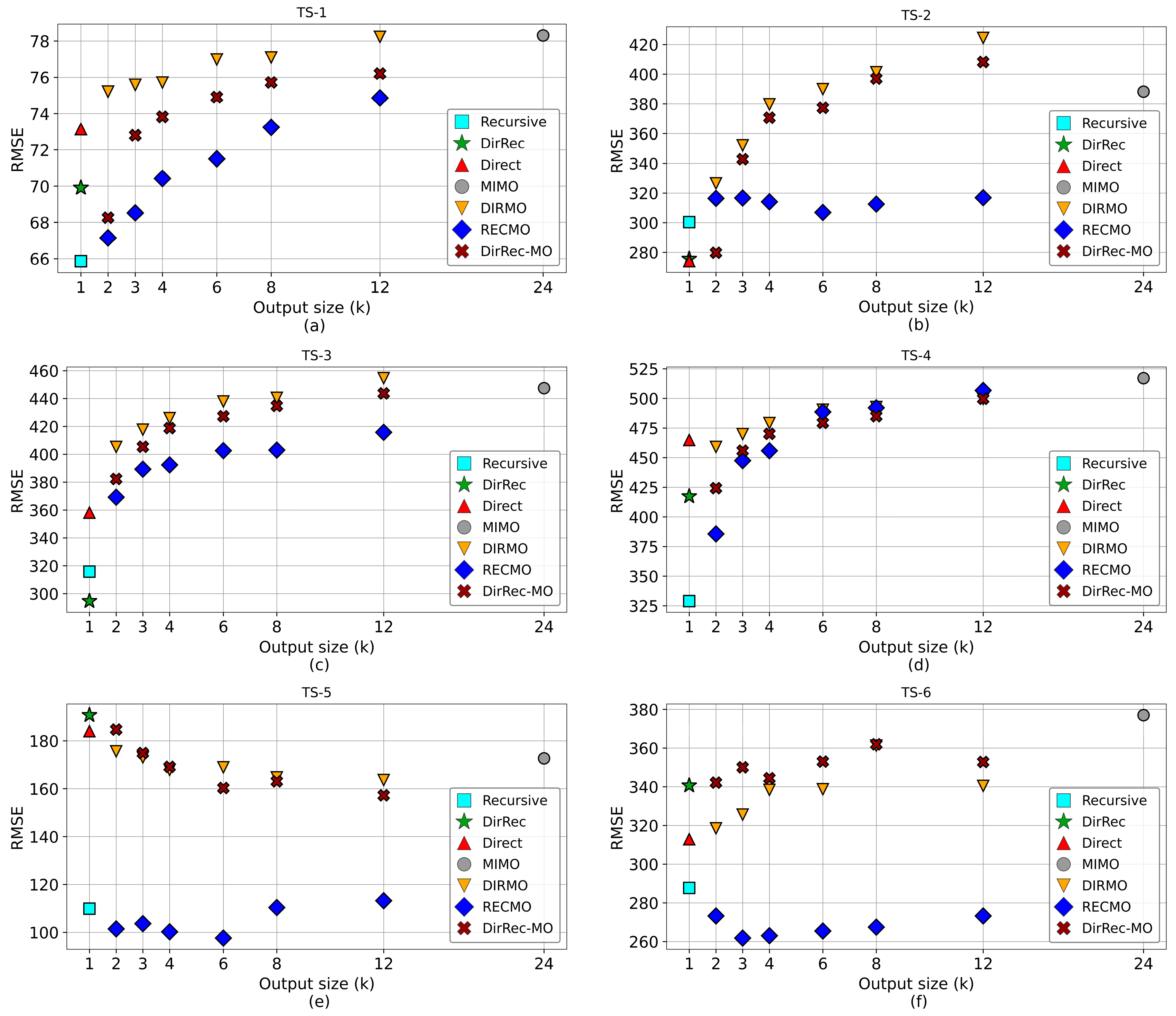
To systematically compare the RMSE values both among different methods and within methods across various multi-outputs, we conducted statistical analyses using Analysis of Variance (ANOVA) and Multivariate Analysis of Variance (MANOVA). We sought to identify significant differences in the RMSE values due to both the forecasting model (Recursive, Direct, DirRec, MIMO, DIRMO, RECMO, or DirRecMO) and the multi-output size (i.e., the different multi-output values considered when predicting the target horizon).
The variability in the RMSE across forecast replications employing different multi-output values (k) and methods was quantified using coefficients of variation (CVs). These coefficients represent the relationship between the standard deviation and the mean. In essence, this ratio measures the extent to which RMSE values carry across forecasting replications, offering insights into the model’s reproducibility and the degree of uncertainty in its replicability. We classified reproducibility as excellent (<10% CV), good (10–20% CV), acceptable (20–30% CV), and poor (>30% CV), based on established recommendations [
44].


