
Ensemble Learning with Highly Variable Class-Based Performance

 , , ,
, , ,
Abstract
:1. Introduction
2. Materials and Methods
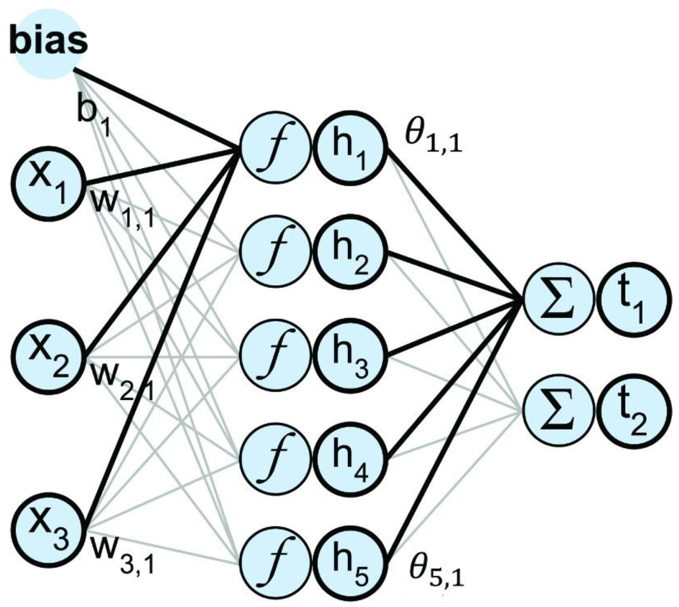
2.1. Extreme Learning Machines
2.2. ELM Ensembles
2.3. Ensemble Model Parameters
2.4. Simple Voting Ensemble
2.5. Weighted Majority Voting Ensemble (WMVE)
2.6. Class-Specific Soft Voting (CSSV) Ensemble
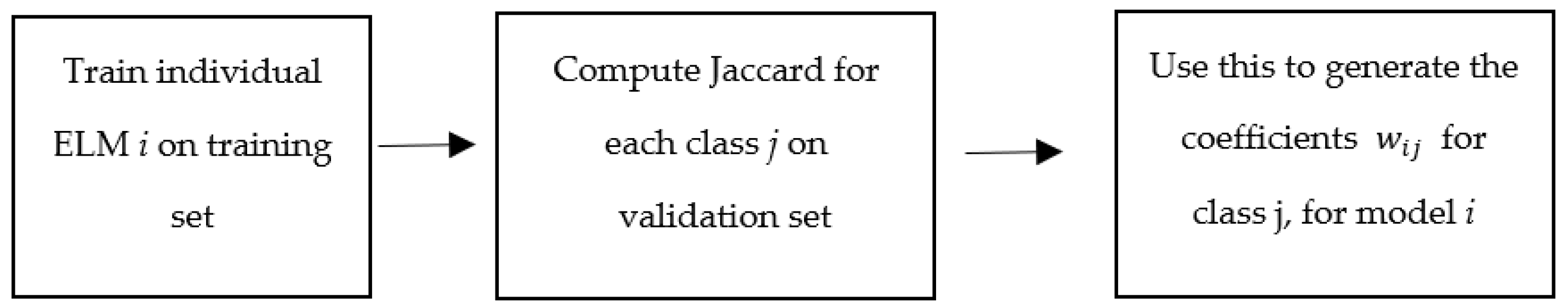
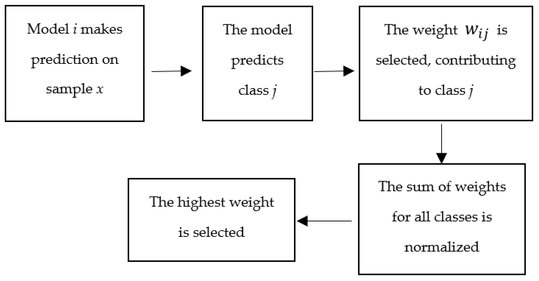
2.7. Novel Class-Based Weighted Ensemble System
2.8. Benchmarking Approach
2.9. Datasets
3. Results
4. Discussion
5. Limitations
6. Patents
Author Contributions
Funding
Data Availability Statement
Conflicts of Interest
References
- Freund, Y.; Schapire, R.E. Experiments with a new boosting algorithm. In Proceedings of the 13th International Conference on Machine Learning ICML, Bari, Italy, 3–6 July 1996; Volume 96. [Google Scholar]
- Breiman, L. Bagging predictors. Mach. Learn. 1996, 24, 123–140. [Google Scholar] [CrossRef]
- Breiman, L. Random forests. Mach. Learn. 2001, 45, 5–32. [Google Scholar] [CrossRef]
- Ho, T.K. Random decision forests. In Proceedings of the 3rd Internal Conference on Document Analysis and Recognition, Montreal, QC, Canada, 14–16 August 1995; Volume 1, pp. 278–282. [Google Scholar]
- Friedman, J.H. Stochastic gradient boosting. Comput. Stat. Data Anal. 2002, 38, 367–378. [Google Scholar] [CrossRef]
- Yang, Q.; Wu, X. 10 challenging problems in data mining research. Int. J. Inf. Technol. Decis. Mak. 2006, 5, 597–604. [Google Scholar] [CrossRef]
- Opitz, D.W.; Shavlik, J.W. Actively searching for an effective neural network ensemble. Connect. Sci. 1996, 8, 337–354. [Google Scholar] [CrossRef]
- Deng, H.; Rnger, G.; Tuv, E.; Vladimir, M. A time series forest for classification and feature extraction. Inf. Sci. 2013, 239, 142–153. [Google Scholar] [CrossRef]
- Bi, Y. The impact of diversity on the accuracy of evidential classifier ensembles. Int. J. Approx. Reason. 2012, 53, 584–607. [Google Scholar] [CrossRef]
- Chen, Z.; Duan, J.; Kang, L.; Qiu, G. Class-imbalanced deep learning via a class-balanced ensemble. IEEE Trans. Neural Netw. Learn. Syst. 2021, 33, 5626–5640. [Google Scholar] [CrossRef]
- Parvin, H.; Mineai, B.; Alizadeh, H.; Beigi, A. A novel classifier method based on class weighting in huge dataset. In 8th Inernational Symposium on Neural Networks, ISNN 2011, Guilin, China, 29 May–1 June 2011; Proceedings, Part II; Springer: Berlin/Heidelberg, Germany, 2011; Volume 8, pp. 144–150. [Google Scholar]
- Ruta, D.; Gabrys, B. Classifier selection for majority voting. Inf. Fusion 2005, 6, 63–81. [Google Scholar] [CrossRef]
- Rojarath, A.; Songpan, W.; Pong-inwong, C. Improved ensemble learning for classification techniques based on majority voting. In Proceedings of the 2016 7th IEEE International Conference on Software Engineering and Service Science (ICSESS), Beijing, China, 26–28 August 2016; pp. 107–110. [Google Scholar]
- Kuncheva, L.I.; Rodriguez, J.J. A weighted voting framework for classifiers ensembles. Knowl. Inf. Syst. 2014, 38, 259–275. [Google Scholar] [CrossRef]
- Dogan, A.; Birant, D. A weighted majority voting ensemble approach for classification. In Proceedings of the 4th International Conference on Computer Science and Engineering (UBMK), Samsun, Türkiye, 11–15 September 2019; pp. 1–6. [Google Scholar]
- Cao, J.J.; Kwong, R.; Wang, R.; Li, K.; Li, X. Class-specific soft voting based multiple extreme learning machines ensemble. Neurocomputing 2015, 149, 275–284. [Google Scholar] [CrossRef]
- Warner, B.; Ratner, E.; Lendasse, A. Edammo’s extreme AutoML technology—Benchmarks and analysis. In International Conference on Extreme Learning Machine; Springer: Berlin/Heidelberg, Germany, 2021; pp. 152–163. [Google Scholar]
- Khan, K.; Ratner, E.; Ludwig, R.; Lendasse, A. Feature bagging and extreme learning machines: Machine learning with severe memory constraints. In Proceedings of the 2020 International Joint Conference on Neural Networks (IJCNN), Glasgow, UK, 19–24 July 2020; IEEE: Piscataway, NJ, USA, 2020; pp. 1–7. [Google Scholar]
- Huang, G.B.; Zhu, Q.Y.; Siew, C.K. Extreme learning machine: Theory and applications. Neurocomputing 2006, 70, 489–501. [Google Scholar] [CrossRef]
- Huang, G.B.; Zhou, H.; Ding, X.; Zhang, R. Extreme learning machine for regression and multiclass classification. IEEE Trans. Syst. Man Cybern. 2009, 42, 513–529. [Google Scholar] [CrossRef] [PubMed]
- Lan, Y.; Soh, Y.C.; Huang, G.B. Ensemble of online sequential extreme learning machine. Neurocomputing 2009, 72, 3391–3395. [Google Scholar] [CrossRef]
- Liu, N.; Wang, H. Ensemble based extreme learning machine. IEEE Signal Process. Lett. 2010, 17, 754–757. [Google Scholar]
- Wang, H.; He, Q.; Shang, T.; Zhuang, F.; Shi, Z. Extreme learning machine ensemble classifier for large-scale data. In Proceedings of the ELM 2014, Singapore, 8–10 December 2014; Springer: Berlin/Heidelberg, Germany, 2014; Volume 1. [Google Scholar]
- Cheng, S.; Yan, J.W.; Zhao, D.F.; Wang, H.M. Short-term load forecasting method based on ensemble improved extreme learning machine. J. Xian Jiaotong Univ. 2009, 43, 106–110. [Google Scholar]
- Huang, S.; Wang, B.; Qiu, J.; Yao, J.; Wang, G.; Yu, G. Parallel ensemble of online sequential extreme learning machine based on MapReduce. Neurocomputing 2016, 174, 352–367. [Google Scholar] [CrossRef]
- Dean, J.; Ghemawat, S. MapReduce: Simplified data processing on large clusters. Commun. ACM 2008, 51, 107–113. [Google Scholar] [CrossRef]
- Wang, G.; Li, P. Dynamic Adaboost ensemble extreme learning machine. In Proceedings of the 2010 3rd International Conference on Advanced Computer Theory and Engineering (ICACTE), Chengdu, China, 20–22 August 2010; Volume 3, pp. V3–54. [Google Scholar]
- Cao, J.; Hao, J.; Lai, X.; Vong, C.M.; Luo, M. Ensemble extreme learning machine and sparse representation classification. J. Frankl. Inst. 2016, 353, 4526–4541. [Google Scholar] [CrossRef]
- Huang, K.; Aviyente, S. Sparse representation for signal classification. In Advances in Neural Information Processing Systems 19, Proceedings of the 2006 Conference, Vancouver, BC, Canada, 4–7 December 2006; MIT Press: Cambridge, MA, USA, 2006; Volume 19, p. 19. [Google Scholar]
- Cao, J.; Lin, Z.; Huang, G.B.; Liu, N. Voting based extreme learning machine. Inf. Sci. 2012, 185, 66–77. [Google Scholar] [CrossRef]
- Martinez-Munoz, G.; Hernandez-Lobato, D.; Suarez, A. An analysis of ensemble pruning techniques based on ordered aggregation. IEEE Trans. Pattern Anal. Mach. Intell. 2008, 31, 245–259. [Google Scholar] [CrossRef] [PubMed]
- Zhang, L.; Zhou, W.D. Sparse ensembles using weighted combination methods based on linear programming. Pattern Recognit. 2011, 44, 97–106. [Google Scholar] [CrossRef]
- Grove, A.J.; Schuurmans, D. Boosting is the limit: Maximizing the margin of learned ensembles. In Proceedings of the AAI/IAAI 98, Madison, WI, USA, 26–30 July 1998; pp. 692–699. [Google Scholar]
- Chen, H.; Tino, P.; Yao, X. A probabilistic ensemble pruning algorithm. In Proceedings of the Sixth IEEE Internal Conference on Data Mining-Workshops (ICDMW’06), Hong Kong, China, 18–22 December 2006; pp. 878–882. [Google Scholar]
- Fletcher, S.; Islam, M.Z. Comparing sets of patters with the Jaccard Index. Australas. J. Inf. Syst. 2018, 22. [Google Scholar] [CrossRef]
- Siegler, R. Balance Scale. In UCI Machine Learning Repository; UC Irvine: Irvine, CA, USA, 1994. [Google Scholar]
- Lim, T.S. Contraceptive Method Choice. In UCI Machine Learning Repository; UC Irvine: Irvine, CA, USA, 1997. [Google Scholar]
- Alcock, R. Synthetic Control Chart Time Series. In UCI Machine Learning Repository; UC Irvine: Irvine, CA, USA, 1999. [Google Scholar]
- Bohanec, M. Car evaluation. In UCI Machine Learning Repository; UC Irvine: Irvine, CA, USA, 1997. [Google Scholar]
- Reyes-Ortiz, J.; Anguita, D.; Ghio, A.; Oneto, L.; Parra, X. Human Actvity Recognition Using Smartphones. In UCI Machine Learning Repository; UC Irvine: Irvine, CA, USA, 2012. [Google Scholar]
- Realinho, V.; Martins, M.; Machado, J.; Baptista, L. Predict Students’ Dropout and Academic Success. In UCI Machine Learning Repository; UC Irvine: Irvine, CA, USA, 2021. [Google Scholar]
- Ciarelli, P.; Oliveira, E. CNAE-9. In UCI Machine Learning Repository; UC Irvine: Irvine, CA, USA, 2012. [Google Scholar]
- Fisher, R.A. Iris. In UCI Machine Learning Repository; UC Irvine: Irvine, CA, USA, 1988. [Google Scholar]

| Dataset | Min # of Neurons | Mid # of Neurons | Max # of Neurons |
|---|---|---|---|
| Balance scale | 10 | 29 | 84 |
| Synthetic control | 10 | 42 | 180 |
| Contraceptive method choice | 10 | 38 | 147 |
| Car evaluation | 10 | 42 | 173 |
| Activity recognition | 10 | 129 | 1683 |
| Student success | 10 | 67 | 442 |
| CNAE9 | 10 | 74 | 540 |
| Iris | 10 | 12 | 15 |
| Dry bean | 10 | 117 | 1361 |
| Yeast | 10 | 39 | 148 |
| Dataset | # Instances | # Features | # Classes | Normalized Class St.dev. |
|---|---|---|---|---|
| Balance scale | 839 | 23 | 3 | 0.6623 |
| Synthetic control | 600 | 60 | 6 | 0.00 |
| Contraceptive method choice | 1473 | 9 | 9 | 0.3035 |
| Car evaluation | 1728 | 6 | 4 | 1.2495 |
| Activity recognition | 10,299 | 561 | 6 | 0.1362 |
| Student success | 4424 | 36 | 3 | 0.4808 |
| CNAE9 | 1080 | 856 | 9 | 0.00 |
| Iris | 150 | 4 | 3 | 0.000 |
| Dry bean | 13,610 | 15 | 7 | 0.4951 |
| Yeast | 1483 | 9 | 10 | 1.1711 |
| Dataset | CSSV | Class (Ours) | WMVE | Single Vote |
|---|---|---|---|---|
| Balance | ||||
| Accuracy | 0.9073 | 0.9186 | 0.9169 | 0.9169 |
| F1 score | 0.7475 | 0.7499 | 0.7319 | 0.7319 |
| Precision | 0.8521 | 0.8584 | 0.8305 | 0.8305 |
| Recall | 0.7289 | 0.7322 | 0.7122 | 0.7122 |
| Avg. Jaccard | 0.8345 | 0.8507 | 0.8478 | 0.8478 |
| Synthetic | ||||
| Accuracy | 0.9233 | 0.9633 | 0.9523 | 0.9456 |
| F1 score | 0.9225 | 0.9629 | 0.9523 | 0.9456 |
| Precision | 0.9219 | 0.9657 | 0.9564 | 0.9423 |
| Recall | 0.9106 | 0.9564 | 0.9533 | 0.9416 |
| Avg. Jaccard | 0.8606 | 0.9297 | 0.9115 | 0.8997 |
| CMC | ||||
| Accuracy | 0.5438 | 0.5275 | 0.5275 | 0.5268 |
| F1 score | 0.5257 | 0.5161 | 0.5161 | 0.5154 |
| Precision | 0.5216 | 0.5214 | 0.5214 | 0.5208 |
| Recall | 0.5300 | 0.5294 | 0.5294 | 0.5282 |
| Avg. Jaccard | 0.3624 | 0.3593 | 0.3592 | 0.3585 |
| Car | ||||
| Accuracy | 0.9456 | 0.9138 | 0.9103 | 0.9051 |
| F1 score | 0.8777 | 0.8417 | 0.8357 | 0.8269 |
| Precision | 0.9114 | 0.9096 | 0.9064 | 0.8991 |
| Recall | 0.8315 | 0.8244 | 0.8260 | 0.8112 |
| Avg. Jaccard | 0.8973 | 0.8417 | 0.8357 | 0.8269 |
| Activity recognition | ||||
| Accuracy | 0.9494 | 0.9501 | 0.9501 | 0.9423 |
| F1 score | 0.8697 | 0.8735 | 0.8735 | 0.8613 |
| Precision | 0.9178 | 0.9213 | 0.9213 | 0.9115 |
| Recall | 0.9101 | 0.9134 | 0.9134 | 0.9090 |
| Avg. Jaccard | 0.9037 | 0.9050 | 0.9050 | 0.8909 |
| Student success | ||||
| Accuracy | 0.7511 | 0.7468 | 0.7462 | 0.7455 |
| F1 score | 0.6736 | 0.6723 | 0.6708 | 0.6695 |
| Precision | 0.6895 | 0.6888 | 0.6877 | 0.6787 |
| Recall | 0.6704 | 0.6652 | 0.6638 | 0.6589 |
| Avg. Jaccard | 0.6018 | 0.5965 | 0.5956 | 0.5948 |
| CNAE-9 | ||||
| Accuracy | 0.8463 | 0.9194 | 0.9167 | 0.9093 |
| F1 score | 0.8484 | 0.9204 | 0.9171 | 0.9104 |
| Precision | 0.8874 | 0.9312 | 0.9273 | 0.9185 |
| Recall | 0.8715 | 0.9194 | 0.9167 | 0.9058 |
| Avg. Jaccard | 0.7350 | 0.8516 | 0.8468 | 0.8348 |
| Iris | ||||
| Accuracy | 0.9400 | 0.9467 | 0.9467 | 0.9467 |
| F1 score | 0.9385 | 0.9458 | 0.9458 | 0.9458 |
| Precision | 0.9485 | 0.9549 | 0.9549 | 0.9549 |
| Recall | 0.9359 | 0.9467 | 0.9467 | 0.9467 |
| Avg. Jaccard | 0.8904 | 0.9029 | 0.9029 | 0.9029 |
| Dry Bean | ||||
| Accuracy | 0.9255 | 0.9258 | 0.9254 | 0.9249 |
| F1 Score | 0.9392 | 0.9391 | 0.9389 | 0.9382 |
| Precision | 0.9355 | 0.9356 | 0.9353 | 0.9349 |
| Recall | 0.9370 | 0.9371 | 0.9368 | 0.9329 |
| Avg. Jaccard | 0.8837 | 0.8840 | 0.8836 | 0.8789 |
| Yeast | ||||
| Accuracy | 0.5400 | 0.5381 | 0.5280 | 0.5219 |
| F1 Score | 0.5015 | 0.4936 | 0.4943 | 0.4889 |
| Precision | 0.5360 | 0.5322 | 0.5358 | 0.5298 |
| Recall | 0.4936 | 0.4936 | 0.4924 | 0.4901 |
| Avg. Jaccard | 0.3766 | 0.3735 | 0.3765 | 0.3701 |
| Dataset | CSSV | Class (Ours) | WMVE | Single Vote |
|---|---|---|---|---|
| Balance | 4 | 1 | 2 | 3 |
| Synthetic | 4 | 1 | 2 | 3 |
| CMC | 1 | 2 | 2 | 4 |
| Car | 1 | 2 | 3 | 4 |
| Activity recognition | 3 | 1 | 1 | 4 |
| Student | 1 | 2 | 3 | 4 |
| CNAE9 | 4 | 1 | 2 | 3 |
| Iris | 4 | 1 | 1 | 1 |
| Dry bean | 2 | 1 | 3 | 4 |
| Yeast | 1 | 2 | 3 | 4 |
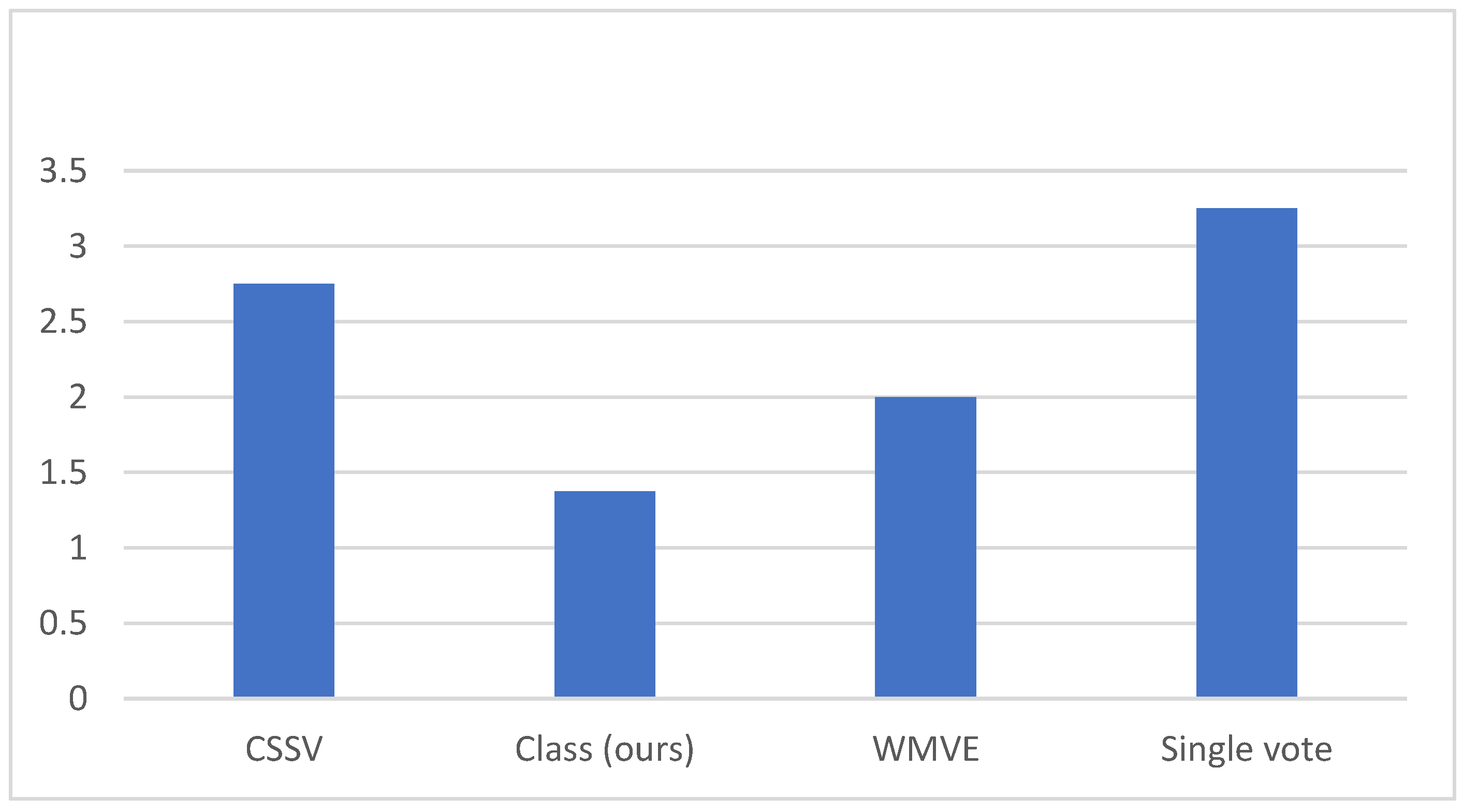
| Average rank | 2.5 | 1.4 | 2.2 | 3.4 |
Disclaimer/Publisher’s Note: The statements, opinions and data contained in all publications are solely those of the individual author(s) and contributor(s) and not of MDPI and/or the editor(s). MDPI and/or the editor(s) disclaim responsibility for any injury to people or property resulting from any ideas, methods, instructions or products referred to in the content. |
© 2024 by the authors. Licensee MDPI, Basel, Switzerland. This article is an open access article distributed under the terms and conditions of the Creative Commons Attribution (CC BY) license (https://creativecommons.org/licenses/by/4.0/).
Share and Cite
Warner, B.; Ratner, E.; Carlous-Khan, K.; Douglas, C.; Lendasse, A. Ensemble Learning with Highly Variable Class-Based Performance. Mach. Learn. Knowl. Extr. 2024, 6, 2149-2160. https://doi.org/10.3390/make6040106
Warner B, Ratner E, Carlous-Khan K, Douglas C, Lendasse A. Ensemble Learning with Highly Variable Class-Based Performance. Machine Learning and Knowledge Extraction. 2024; 6(4):2149-2160. https://doi.org/10.3390/make6040106
Chicago/Turabian StyleWarner, Brandon, Edward Ratner, Kallin Carlous-Khan, Christopher Douglas, and Amaury Lendasse. 2024. "Ensemble Learning with Highly Variable Class-Based Performance" Machine Learning and Knowledge Extraction 6, no. 4: 2149-2160. https://doi.org/10.3390/make6040106