Tutorial

Deep Learning with Convolutional Neural Networks: A Compact Holistic Tutorial with Focus on Supervised Regression

by
Yansel Gonzalez Tejeda
* and
Helmut A. Mayer
Department of Artificial Intelligence and Human Interfaces, Paris Lodron University of Salzburg, 5020 Salzburg, Austria
*
Author to whom correspondence should be addressed.
Mach. Learn. Knowl. Extr. 2024, 6(4), 2753-2782; https://doi.org/10.3390/make6040132
Submission received: 26 August 2024 / Revised: 21 November 2024 / Accepted: 22 November 2024 / Published: 30 November 2024
(This article belongs to the Section Learning)

Abstract

:
In this tutorial, we present a compact and holistic discussion of Deep Learning with a focus on Convolutional Neural Networks (CNNs) and supervised regression. While there are numerous books and articles on the individual topics we cover, comprehensive and detailed tutorials that address deep learning from a foundational yet rigorous and accessible perspective are rare. Most resources on CNNs are either too advanced, focusing on cutting-edge architectures, or too narrow, addressing only specific applications like image classification. This tutorial not only summarizes the most relevant concepts but also provides an in-depth exploration of each, offering a complete yet agile set of ideas. Moreover, we highlight the powerful synergy between learning theory, statistics, and machine learning, which together underpin the deep learning and CNN frameworks. We aim for this tutorial to serve as an optimal resource for students, professors, and anyone interested in understanding the foundations of deep learning.

1. Introduction

In this tutorial, we discuss the theoretical foundations of Artificial Neural Networks (ANNs) in their variants with several intermediate layers, namely deep artificial neural networks. More specifically, we focus on particular ANNs known as Convolutional Neural Networks (CNNs).
In order to introduce the methods and artifacts we will use, we mostly follow the classical literature on Artificial Intelligence (AI) from an overall perspective [1] and Deep Learning (DL) [2]. We begin by motivating DL in Section 2 and enunciating its standard taxonomy. Since ANNs are learning systems, we first expose Machine Learning (ML) concepts in Section 3. We then discuss the general structure of an ANN (Section 4) and the concept of depth in that context. Convolutional neural networks are named as such because convolutions are a key building block of their architecture. For that reason, in Section 5, we incorporate the convolution operation to complete our exposition of CNNs. Finally, in Section 6, we summarize the more relevant facts.
The theoretical deep learning framework is immense and has many ramifications to learning theory, probability and statistics, optimization, and even cognitive theory, to  mention just a few examples. There are several books for every topic described in the subsections of this tutorial, as well as in conferences and journals. Therefore, our presentation of deep learning here is highly selective and aims to expose the fundamental aspects needed for agile assimilation of DL.
It is worth noting that since DL is a relatively young field, the  terminology greatly varies. We often indicate when several terms are used to designate a concept, but the reader should be aware that this indication is by far not exhaustive. Notation is at the end of this manuscript.
We provide an accompanying repository at https://github.com/neoglez/deep-learning-tutorial.

2. Motivation

Intelligent agents need to learn in order to acquire knowledge from their environment. To perform various tasks, humans learn, among other things, from examples. In this context, learning means that for a defined task, the agent must be able to generalize. That is, the agent should successfully perform the task beyond the examples it has seen before, and typically, we expect the agent to make some form of prediction. Most tasks the agent performs can be framed as either classification or regression. For both types of tasks, when the examples are accompanied by known target values or labels, which the agent aims to predict, we refer to this as supervised learning, as a learning paradigm. From a pedagogical perspective, the agent is being supervised by receiving the ground truth corresponding to each learning example.
In addition to supervised learning, there are three other learning paradigms: unsupervised learning, reinforcement leaning, and semi-supervised learning. When no targets are available, or targets are not provided, learning must occur in an unsupervised manner. If, alternatively, the targets are noisy or some are missing, learning must proceed in a semi-supervised manner. In contrast, if no ground truth is provided at all, but a series of reinforcements can be imposed, the agent can nonetheless learn by being positively or negatively (punished) rewarded. Here, we focus on supervised learning.

3. Machine Learning

From a general perspective, the learning agent has access to a set of ordered examples:
X = def { x ( 1 ) , , x ( m ) }
which are assumed to have been drawn from some unknown generating distribution  p d a t a . A learning example  x ( i )  (also a pattern) may be anything that can be represented in a computer; for example, a scalar, a text excerpt, an image, or a song. Without loss of generality, we will assume that every  x ( i )  is a vector  x ( i ) R n , and its components are the example features. For instance, one could represent an image as a vector by arranging its pixels to form a sequence. Similarly, a song could be vectorized by forming a sequence of its notes. We will clarify when we refer to a different representation.
Furthermore, the examples are endowed with their ground truth (set of labels, also supervision signal Y  so that for every example  x ( i ) , there exists a label (possibly a vector)  y i Y . Using these examples, the agent can learn to perform two types of tasks: regression and classification (or both). Regression may be defined as estimating one or more values  y R ; for  instance, human body dimensions like height or waist circumference. In a classification scenario, the agent is required to assign one or more of a finite set of categories to every input; for example, from an image of a person, designate which body parts are arms or legs.
Additionally, in single-task learning, the agent must learn to predict a single quantity (binary or multi-class classification, univariate regression), while in multi-task learning, the algorithm must learn to estimate several quantities, e.g.,  multivariate multiple regression.

3.1. Learning Theory

In general, we consider a hypothesis space  H , consisting of functions. For example, one could consider the space of linear functions. Within  H , the function
f ( X ) = Y
maps the examples (inputs) to their labels (outputs). The learning agent can be then expressed as a model
f ^ ( X ) = Y ^
that approximates f, where  Y ^  is the model estimate of the targets  Y .
Now, the ultimate goal of the learning agent is to perform well beyond the examples it has seen before, i.e., to exhibit good generalization. More concretely, learning must have low generalization error. To  assess generalization, the stationarity assumption must be adopted to connect the observed examples to the hypothetical future examples that the agent will perceive. This assumption postulates that the examples are sampled from a probability distribution  p d a t a  that remains stationary over time. Additionally, it is assumed that (a) each example  x ( i )  is independent of the previous examples, and (b) that all examples have identical prior probability distributions, abbreviated i.i.d..
With this in hand, we can confidently consider the observed examples as a training set  { x t r a i n , y t r a i n }  (also training data) and the future examples as a test set  { x t e s t , y t e s t } , where generalization will be assessed. As the data generating distribution  p d a t a  are assumed to be unknown (we will delve into this in Section 3.3), the  agent only has access to the training set. One intuitive strategy for the learning agent to estimate generalization error is to minimize the training error computed on the training set, also termed empirical error or empirical risk. Thus, this strategy is called empirical risk minimization (ERM). Similarly, the test error is calculated on the test set. Both training and test errors are defined in a general form as the sum of incorrect estimated targets by the model (in Section 3.4.1, we restate this definition); for  example, in the case of m training examples, the training error  E t r a i n  is as follows:
E t r a i n = i = 1 m f * ( x ( i ) ) y i .
Note that given a specific model  f * , based on the i.i.d. assumption, the expected training error equals the expected test error. In practice, the previous is greater than or equal to the latter. Here, the model may exhibit two important flaws: underfitting or overfitting. A model that underfits does not achieve a small training error (it is said that it cannot capture the underlying structure of the data). Overfitting is the contrary of underfitting; it occurs when the model “memorizes” the training data, “perhaps like the everyday experience that a person who provides a perfect detailed explanation for each of his single actions may raise suspicion” [3]. When evaluated, a model that underfits yields a high difference between the training and the test error.

3.2. Model Evaluation

Assessing generalization by randomly splitting the available data into a training set and a test set is called holdout cross-validation because the test set is kept strictly separate from the training set and used only once to report the algorithm’s results. However, this model evaluation technique has two important disadvantages:
  • It does not use all the data at hand for training; a problem that is specially relevant for small datasets.
  • In practice, there can be cases where the i.i.d. assumption does not hold. Therefore, the assessment is highly sensitive to the training/test split.
A remedy to these problems is the k-fold cross-validation evaluation method (cf. [4] (p. 241)—Cross Validation). It splits the available data into k non-overlapping subsets of equal size. Recall that the dataset has m examples. First, learning is performed k times with  k 1  subsets. Second, in every iteration, the test error is calculated on the subset that was not used for training. Finally, the model performance is reported as the average of the k test errors. The cost of using this method is the computational overload, since training and testing errors must be computed k times.

3.3. Statistics and Probability Theory

To further describe machine learning, we borrow statistical concepts. In order to be consistent with the established literature [2], we use in this subsection  θ  and  θ ^  to to denote a quantity and its estimator.
The agent must learn to estimate the wanted quantity, e.g.,  θ . From  a statistical perspective, the agent performs a point estimate  θ ^ . In  this view, the data points are the i.i.d. learning examples  { x ( 1 ) , , x ( m ) } . A  point estimator is a function of the data such as  θ ^ m = def g ( { x ( 1 ) , , x ( m ) } ) , with  g ( x )  being a very general suitable function. Note that we can connect the quantity  θ  and its estimator  θ ^  to the functions f and  f ^  in Equations (2) and (3). Given the hypothesis space  H  that embodies possible input–output relations, the  function  f ^  that approximates f can be treated as a point estimator in function space.
Important properties of estimators are bias, variance, and standard error. The  estimator bias is a measure of how much the real and the estimated values differ. It is defined as  b i a s ( θ ^ m ) = E ( θ ^ m ) θ . Here, the expectation  E  is taken over the data points (examples).
An unbiased estimator has  b i a s ( θ ^ m ) = 0 ; this implies that  θ ^ m = θ . An asymptotically unbiased estimator is when  lim m b i a s ( θ ^ m ) = 0 , which implies that  lim m θ ^ m = θ . An example of an unbiased estimator is the mean estimator (mean of the training examples) of the Bernoulli distribution with mean  θ .
The variance  V a r ( θ ^ ) =  and standard error  S E ( θ ^ )  of the estimator are useful for comparing different experiments. A good estimator has low bias and low variance.
Let us now discuss two important estimators: the maximum Likelihood and the maximum a posteriori estimators.

3.3.1. Maximum Likelihood Estimation

To guide the search for a good estimator  θ ^ , the   frequentist approach  is usually adopted. The wanted quantity  θ , possibly multidimensional, is seen as fixed but unknown, and the observed data are random. The parameters  θ  govern the data generating distribution  p d a t a ( x )  from which the observed i.i.d. data  { x ( 1 ) , , x ( m ) }  arose.
Then, a parametric model for the observed data is presumed, i.e., a probability distribution  p m o d e l ( x ; θ ) . For  example, if the observed data are presumed to have a normal distribution, then the parameters are  θ = { μ , σ } , and the model  p m o d e l ( x ; θ ) = 1 σ 2 π e 1 2 x μ σ 2 . Here, candidates parameters  θ  must be considered, and ideally,  p m o d e l ( x ; θ ) p d a t a ( x ) . Next, a  likelihood function  L can be defined as the mapping between the data  x  and a given  θ  to a real number estimating the true probability  p d a t a ( x ) . Since the observations are assumed to be independent,
L ( x ; θ ) = i = 1 m p m o d e l ( x ( i ) , θ ) .
The Maximum Likelihood (ML) estimator is the estimator  θ ^  that, among all candidates, chooses the parameters that make the observed data most probable.
θ ^ M L = arg   max θ   L ( x ; θ )
= arg   max θ i = 1 m p m o d e l ( x ( i ) , θ )
Taking the logarithm of the right side in 7 facilitates the probability computations and does not change the maximum location. This leads to the  Log - likelihood .  
θ ^ M L = arg   max θ i = 1 m log p m o d e l ( x ( i ) , θ )
An insightful connection to information theory can be established by transforming Equation (8). Firstly, dividing the right term by the constant m does not shift the maximum in the left term, i.e.,
θ ^ M L = arg   max θ 1 m i = 1 m log p m o d e l ( x ( i ) , θ ) .
Secondly, by definition, the empirical mean  1 m i = 1 m log p m o d e l ( x ( i ) , θ )  of the assumed model distribution  p m o d e l  equals the expectation given its empirical distribution  E X p ^ d a t a  defined by the training set  p ^ d a t a ( x ) . A discussion of the empirical distribution  p ^ d a t a ( x )  is out of this scope, but it is a method used to approximate the real underlying distribution of the training set (not to be confused with the data-generating distribution  p d a t a ). Finally, Equation (9) can be written as follows:
θ ^ M L = arg   max θ E X p ^ d a t a log p m o d e l ( x , θ ) .
Information theory allows us to evaluate the degree of dissimilarity between the empirical distribution of the training data  p ^ d a t a ( x )  and the assumed model distribution  p m o d e l ( x )  using the Kullback–Leibler divergence  D K L  (also called relative entropy) as follows:
D K L ( p ^ d a t a p m o d e l ) = E x p ^ d a t a [ log p ^ d a t a ( x ) log p m o d e l ( x ) ] .
Here, the expectation  E  is taken over in the training set because Equation (11) quantifies the additional uncertainty arising from using the assumed model  p m o d e l  to predict the training set  p ^ d a t a .
Because we want the divergence between these two distributions to be as small as possible, it makes sense to minimize  D K L . Note that the term  log p ^ d a t a ( x )  in Equation (11) can not be influenced by optimization, since it has been completely determined by the data-generating distribution  p d a t a . We denote the minimum  D K L  as  θ D K L , then
θ D K L = arg   min θ E x p ^ d a t a [ log p m o d e l ( x , θ ) ]
The expression inside the arg min is the cross-entropy of  p ^ d a t a  and  p m o d e l . Comparing this with Equation (10), we arrive at the conclusion that maximizing the likelihood coincides exactly with minimizing the cross-entropy between the distributions.

3.3.2. Maximum a Posteriori Estimation

In contrast to the frequestist approach, the Bayesian approach considers  θ  to be a random variable and the dataset  x  to be fixed and directly observed. A prior probability distribution  p ( θ )  must be defined to express the degree of uncertainty of the state of knowledge before observing the data. In the absence of more information, a Gaussian distribution is commonly used. The Gaussian distribution is “the least surprising and least informative assumption to make” [5], i.e., it is the distribution with the maximum entropy. Therefore, the Gaussian distribution is an appropriate starting prior when conducting Bayesian inference.
After observing the data, Bayes’ rule can be applied to find the posterior distribution of the parameters given the data  p ( θ | x ) = p ( x | θ ) p ( θ ) p ( x ) , where  p ( x | θ )  is the likelihood and  p ( x )  the probability of the data.
Then, the Maximum a Posteriori (MAP) estimator selects the point of maximal posterior probability:
θ ^ M A P = arg   max θ   p ( θ | x ) = arg   max θ   l o g p ( x | θ ) + l o g p ( θ ) .

3.4. Optimization and Regularization

3.4.1. Loss Function

The training error, as defined by Equation (4), is an objective function (also criterion) that needs to be minimized. Utility theory regards this objective as a loss function  J ( x ) : R n R , because the agent incurs a loss of expected utility when estimating the wrong output with respect to the expected utility when estimating the correct value. To  establish the difference between these values, a determined distance function must be chosen.
For general (multivariate, multi-target) regression tasks, the p-norm is preferred. The p-norm is calculated on the vector of the corresponding training or test error  y ^ i y i p = i | y ^ i y i | p 1 p , which for  p = 2  reduces to the Euclidean norm. Since the Mean Squared Error (MSE)  y ^ i y i 2 2  can be computed faster, it is often used for optimization. We used this loss function (also cost function) when training our network (2) with m examples:
J ( y ) = 1 m i = 1 m y ^ i y i 2
= 1 m i = 1 m 1 2 j = i | y | y ^ j y j 2 .
Since we regard every target  y i  as a vector, the inner sum runs over its components  y i , and  | y |  is its length. The rather arbitrary scaling factor 2 in the denominator is a mathematical convenience for the discussion in Section 4.2.
For classification tasks, the cross-entropy loss is commonly adopted.

3.4.2. Gradient-Based Learning

As we will see in Section 4, in the context of deep learning, the  parameters  θ  discussed in Section 3.3 are named weights  w . Without loss of generalization, we will consider the parameters to be a collection of weights. We do not lose generalization because the discussion here does not depend on the specific form of the cost function.
Therefore, parameterizing the estimator function by the weights, minimization of the cost function can be written as follows:
J * ( w ; x , y ) = arg   min w 1 m i = 1 m f ^ ( x ( i ) , w ) y i 2
The function  f ^ ( x ( i ) , w )  is, in a broader sense, a  nonlinear model; thus, the minimum of the loss function has no closed form, and numeric optimization must be employed. Specifically, J is iteratively decreased in the orientation of the negative gradient, until a local or global minimum is reached, or the optimization converges. This optimization method (also optimizer) is termed gradient descent. Because optimizing in the context of machine learning may be interpreted as learning, a  learning rate  ϵ  is introduced to influence the step size at each iteration. The gradient descent optimizer changes the weights using the gradient  w  of  J ( w )  according to the weight update rule:
w w ϵ w J ( w )
We postpone the discussion on Stochastic Gradients Descent (SGD) to insert it in the context of training neural networks (Section 4.2).

3.4.3. Regularization

The essential problem in machine learning is to design algorithms that perform well both in training and test data. However, because the true data-generating process is unknown, merely decreasing the training error does not guarantee a small generalization error. Even at worst, extremely small training errors may be a symptom of overfitting.
Regularization intends to improve generalization by combating overfitting. It focuses on reducing the test error using constraints and penalties on the model family being trained, which can be interpreted as pursuing a more regular function.
One such important penalty may be incorporated into the objective function. More specifically, the models parameters may be restricted by a function  Ω ( w )  to obtain the modified cost function  J ˜ ( w )  with two terms as follows:
J ˜ ( w ) = arg   min w 1 m i = 1 m f ^ ( x ( i ) , w ) y i 2 + α Ω ( w ) .
The second term’s coefficient  α [ 0 , )  ponders the penalty’s influence relative to  J * . The specific form of  Ω ( w )  (also a regularizer) is usually a  L 1 = w 1  or  L 2 = w 2 2  norm penalty. Choosing one of these norm penalties expresses a preference for a determined function class. For example, the  L 1  penalty enforces sparsity on the weights, i.e., it pushes the weights towards zero, while the effect of the  L 2  norm causes the weights of less-influential features to decay. Because of this, the  L 2  penalty norm is called weight decay.
Weight decay has lost popularity in favor of other regularization techniques (Section 5.5). It worth saying, however, that weight decay is an uncomplicated, effective method for enhancing generalization [6]. Modifying Equation (16) to include the penalty with  α = 1 2 , the cost function becomes the following:
J ˜ ( w ) = arg   min w 1 m i = 1 m f ^ ( x ( i ) , w ) y i 2 + α 2 w T w .
Correspondingly, after substituting and reorganizing terms, the weight update rule in Equation (17) results in the following:
w ( 1 ϵ α ) w ϵ w J ( w ) .

4. Deep Forward Artificial Neural Networks

Deep Forward Artificial Neural Networks (DFANNs) are a model conveying several important interlaced concepts. We start with its building blocks and then connect them to form the network. Additionally, to describe the parts of an ANN, the term architecture is used.

4.1. Artificial Neural Networks

Artificial Neural Networks (ANNs) are a computational model originally inspired by the functioning of the human brain [7,8,9]. The model exploits the structure of the brain, focusing on neural cells (neurons) and their interactions. These neurons have three functionally distinct parts: dendrites, somas, and axons. The dendrites gather information from other neurons and transmit it to the soma. Then, the soma performs a relevant nonlinear operation. If  exceeding a determined threshold, the result causes the neuron to emit an ouput signal. Then, the output signal is delivered by the axon to others neurons.

4.1.1. Artificial Neurons

Similarly, the elementary processing unit of ANNs is an artificial neuron. The  neurons receive a number of inputs with associated intensities (also strengths) and combine these inputs in a nonlinear manner to produce a determined output that is transmitted to other neurons. Depending on the form of the non-linearity, it can be said that the neuron ‘fires’ if a determined threshold is reached.
Every input to the neuron has an associated scalar called weight w. The non-linearity, also called the activation function is denoted by  g ( · ) . The neuron first calculates an affine transformation of its inputs  z = i = 1 n w i · x i + c . The intercept (also bias) c may be combined with a dummy input  x d u m m y = 1  to simplify notation such as the affine transformation, which can be written in matrix form as follows:  i = 0 n w i · x i = w · x . One of the reasons that ANNs were invented was to overcome the limitations of linear models. Since a linear combination of linear units is also linear, a non-linearity is needed to increase the capacity of the model. Accordingly, the neuron applies the activation function to compute the activation  a = g ( w · x ) , which is transmitted to other neurons.
Referring to activation functions, [2] states categorically that “In modern neural networks, the default recommendation is to use the rectified linear unit or ReLU”, introduced by [10] as follows:
g ( z ) = m a x ( 0 , z ) .
In order to enable learning with gradient descent (Equation (17)), as described in Section 3.4.2, it is desirable that the activation function is continuous differentiable. Although the ReLU is not differentiable at  z = 0 , in practice, this does not constitute a problem. Practitioners assume a ‘derivative default value’  f ( 0 ) = 0 f ( 0 ) = 1  or values in between.
Other activation functions are the logistic sigmoid  σ ( z ) = 1 / ( 1 + e x p ( z ) )  and the softplus function ζ ( z ) = log ( 1 + e x p ( z ) ) . As a side note, a neuron must not necessarily compute a non-linearity, and in that case, it is called a linear unit.
The perceptron is an artificial neuron introduced by [9], who demonstrated that only one neuron is sufficient to implement a binary classifier. The perceptron originally had a hard threshold activation function, but it can be generalized to use any of the above-mentioned activation functions. For example, if the perceptron uses a logistic sigmoid activation function, then the output can be interpreted as the probability of some event happening, e.g., logistic regression.

4.1.2. Deep Feedforward Networks

Connecting the artificial neurons results in an artificial neural network with at least two distinguishable layers: the input layer and the output layer. The input layer is composed of the units that directly accept the features (or their preprocessed representation) of the learning examples. The output layer contains the units that produce the answer to the learning task.
A single-layer neural network (sometimes called a single-layer perceptron network, or simply a perceptron network) (SLNN) is the most basic structure that can be assembled by directly connecting any number of input units to any number of output units. Note that, by  convention, the input layer is not counted. Despite this type of network being far from useless, it is limited in its expressive power. Perceptron networks are unable to represent a decision boundary for non-linearly separable problems [11]. A  problem is linearly separable if the learning examples can be separated into two nonempty sets, e.g., every set can be assigned exclusively to one of the two half spaces defined by a hyperplane in its ambient space. This is important because, in general, practical problems in relevant areas like computer vision and natural language processing are not linearly separable.
Beyond the SLNN, networks can be extremely complex. In order to make progress, one important restriction that may be imposed is to model the network as a directed acyclic graph (DAG) with no shortcuts. The neurons are the nodes, the connections are the directed edges (or links), and the weights are the connection intensities. Because  a DAG does not contain cycles, the information in the ANN is said to flow in one direction. For this reason, this type of ANN that does not contain feedback links, which are called feedforward networks or multi-layer perceptrons (MLPs). If the network does have feedback links, then it is called a recurrent neural network (RNN). In this tutorial, we focus on feedforward networks.
In Equation (3) (Section 3), we enunciated that the goal of a learning agent  f ^ ( x )  is to approximate some function  f ( x ) , and from a statistical perspective, the agent is a function estimator of  θ  (Section 3.3). Motivated by the idea of compositionality, it can be assumed that this learning agent  f ^ ( x )  is precisely the composition of a number of different functions:
f ^ ( x ) = f n ( f n 1 ( f 0 ( x ) ) )
where  f ( 0 )  and  f ( n )  represent the input and output layers, respectively.
Furthermore, starting from the input layer and ending at the output layer, every function  f ( l )  for  l 1 , , n 1  can be associated with a collection of DAG units that receive inputs only from the units in preceding collections. These functions and the units group they define are called hidden layers and are denoted by  h ( · ) .
Hidden layers are named as such because of their relation to the training examples. The training examples determine the form and behavior of the input and the output layer. Indeed, the input layer processes the training examples, and the output layer must contribute to minimize the training loss. However, the training examples do not rule the intermediary layer computation scheme. Instead, the algorithm must learn how to adapt those layers to achieve its goal.
Finally, the length of the entire function chain  f ( 1 ) , , f ( n )  is the depth  of the network ( f ( 0 )  is the first layer but is not counted for depth), which, combined with the concepts explained before, confers the name to the computational model: deep feedforward networks. Likewise, the width of a layer is the number of units it contains, and the network’s width is sometimes defined as the “maximal number of nodes in a layer” [12]. Additionally, the input layer is also called the first layer; the next layers are the second, the third, and so forth.
The architecture of the network designates the network’s depth and width, as well as the layers and their connections to each other (in Section 5.1, we show an example of a network architecture). Depending on how the units are connected, different layer types can be assembled. Note that because shortcuts are not allowed, there cannot be intra-layer unit connections. The fully connected layer  h ( l )  (also a dense layer, in  opposition to a shallow layer) is the most basic, where all of its units connect to all of the units of the preceding layer  h ( l 1 )  though a weight matrix  W , i.e.,
h ( l ) = g l ( W l h ( l 1 ) + b l )
h ( l ) = g l ( W l h ( l 1 ) ) .
The weight matrix is  W l R m × n  and the bias vector is  b l R m , where m and n are the widths of the current and preceding layer, respectively. Alternatively, the notation may be simplified by incorporating the bias vector into the matrix with a dummy input (Equation (24)).
In Section 4.2.3, we will further discuss the notation, and in Section 5.1, we will see other layer types.
One of the most significant results in feedforward network research is the universal approximation theorem. The exact form of these theorems is positively technical, but at their core, they demonstrate that feedforward networks can approximate any continuous function to any desirable level of accuracy. There are three theorem variants: arbitrary width and bounded depth, i.e., a universal approximator with only one hidden layer containing a sufficient number of neurons [13]; bounded width and arbitrary depth [14], i.e., a sufficient number of layers with a bounded number of neurons; and remarkably, bounded depth and width [15].

4.2. Training

Having described the structure of an artificial neural network, and how it learn via optimization, we now need to perform the actual training. The learning examples are entered into the network through the input layer, and the network weights need to be updated using gradient descent to minimize the loss.

4.2.1. Stochastic Gradient Descent

As we already discussed in Section 3.4.2, gradient descent enables optimization of general loss functions. Specifically, the model weights are updated using the gradient of the loss function  w J ( w ) , which is sometimes called pure, deterministic, or batch gradient descent. The problem is that the computation of this gradient requires an error summation over the entire dataset  w J ( w ) = i = 1 m ( y ^ i y i ) x i . In practice, this computation can be extremely expensive or directly intractable.
Stochastic gradient descent (SGD) proposes a radical solution to this problem. It does not compute the gradient exactly. Instead, it estimates the gradient with one training example,  x ( i ) . For this reason, SGD can be seen as an online algorithm that processes a stream of steadily produced data points, one example at a time.
As expected, this gradient estimation is highly noisy; an issue that can be alleviated by using not one but a randomly sampled subset of learning examples. This subset is called a mini-batch, and its size n is the batch size, which should not be confused with the above-mentioned deterministic optimizer.
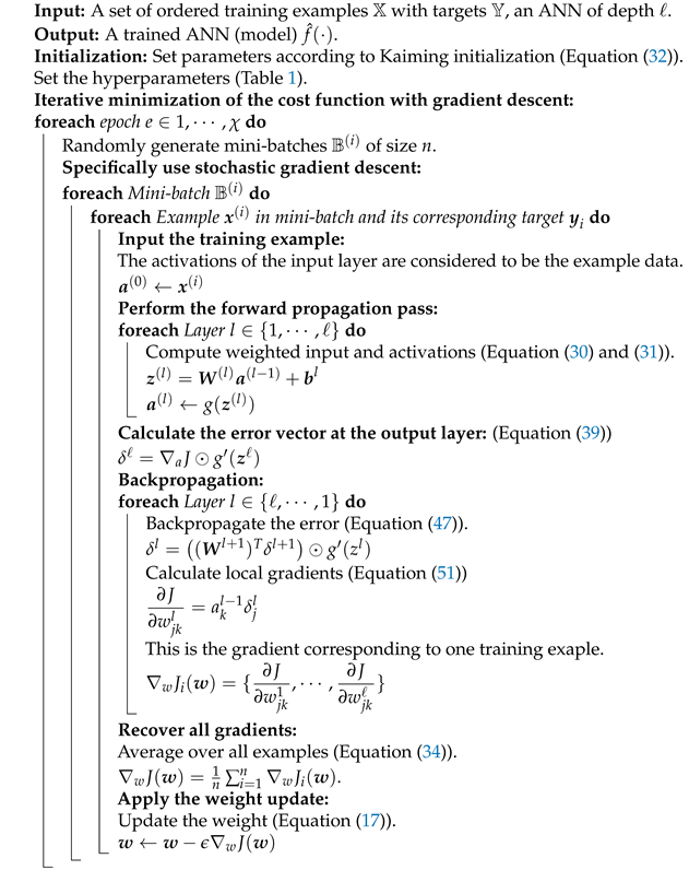
Moreover, SGD has an iterative nature, and when training an ANN, one iteration is called an epoch. In every epoch, the training data are divided into a number of mini-batches. The mini-batches are disjoint subsets of the training set, and the last mini-batch may have fewer examples as n. After the first mini-batch has been used to estimate the gradient, training continues with the next mini-batch, and so forth, until the training data have been completely processed. In this tutorial, the learning agent shown in Algorithm 1 ends after a predefined number of epochs  χ .
Perhaps surprisingly, the strategy of SGD not only accelerates training but improves generalization as well, as concisely stated by [16]: “train faster, generalize better”. Although SGD was first introduced many decades ago by [17], it remains widely used today. For an amenable discussion on SGD recent trends, [18] may be consulted.

4.2.2. SGD with Momentum

Despite the computational and efficacy advantages of SGD, its trajectory to the optimum or an appropriate stationary point can be slow. To overcome this limitation, the momentum algorithm changes the weights, proceeding by incorporating the contribution of preceding gradients. This accelerates learning because strong fluctuations in the gradients can be diminished;  therefore, the path to the minimum is less oscillating.
One can gain intuition into the momentum algorithm by drawing a physical analogy. Let the learning algorithm be a heavy ball rolling down the optimization landscape. The ball is subject to two forces: a gravity-like force acting in the direction of the negative gradient,  w J ( w ) , and a viscous force attenuating its movement, proportional to its velocity v. Therefore, the weights should be updated according to the net force acting on the ball.
In particular, since momentum is mass times velocity, and considering the ball to have unit mass, the velocity can be interpreted as momentum. Then, introducing a term  v  and a parameter  α [ 0 , 1 )  for damping, the weight update can be written as follows:
v α v ϵ w J ( w )
w w + v
Despite the parameter  α  being more related to viscosity, it is widely called the momentum parameter. Furthermore, the velocity update at iteration k can be written as  v k = α k v 0 ϵ i = 0 k 1 α i J w ( w k 1 i ) . Given that  α < 1 , the  velocity accumulates previous gradients and updates the weights using an exponential moving average, where recent gradients have more importance (lower powers of  α ) than previous gradients.
SGD with momentum may be generalized to a family of optimization methods called ‘Linear First Order Methods’ [19], but the presentation here shall be enough for our discussion.

4.2.3. Forward-Propagation and Back-Propagation

In this subsection, we departure from our two main references and follow [20,21].
We are now ready to begin training the network. This requires a proper definition of an individual weight in a certain layer l, i.e., the weight  w j k l  connects the  k t h  neuron in the  ( l 1 ) t h  layer to the  j t h  neuron in the current layer l. This rather intricate notation is necessarily in order to compactly relate the activation of consecutive layers  a l  and  a l 1 :
a j l = g k w j k l a k l 1 + b j l
a l = g ( W l a l 1 + b l ) .
Here, if we fixate the neuron j with weight  w j k l  and bias  b l  at layer l, then its activation  a j l  results from the activation in the preceding layer according to Equation (27). Intuitively, the activation of a neuron is a function of its weighted inputs, i.e., the activation of all the units connected to it from the previous layer and the bias of the neuron (Figure 1). Equation (28) is its vectorized form, where  g ( · )  is the activation function applied element-wise.
Furthermore, the weight sum before applying the non-linearity is called the weighted input  z j l  to neuron j in layer l. It is defined as follows:
z j l = def k w j k l a k l 1 + b j l
z ( l ) = def W ( l ) a ( l 1 ) + b l
a ( l ) = g ( z ( l ) ) .
Equation (30) is the weighted input in vectorized form, and Equation (31) is the activation written as a function of the weighted input.
Training requires initialization of the weights and the bias. More importantly, appropriate weight initialization is crucial for convergence. The general idea is to break the symmetry among the units such that every node computes a different function. Although there are several initialization strategies, usually, the weights are drawn randomly from a Gaussian or uniform distribution.
However, due to the chain nature of ANNs, two problems might arise: vanishing gradients or exploiting gradients. If  the weights are initialized with extremely small values, e.g., from a Gaussian with zero mean and std.  0.01 , the hidden layer activations may tend to zero. Therefore, the gradient of the cost function may vanish. Exactly the contrary might happen if the weights are initialized with relatively high values (it suffices with an increase in the above-mentioned std. to  0.05 ), which might lead to exceedingly large gradients. Both vanishing and exploiting gradients hinder learning. In general, the  problem is that large weight variance can render learning unstable.
Kaiming initialization [22] (also He initialization) attempts to avoid learning instability by constraining the weight variance to be nearly constant across all layers. This strategy was first proposed by [23], but the derivation did not contemplate ReLU. Concretely, the heuristic is to derive the relation by enforcing that the contiguous layers have equal output variance  V a r ( a ( l ) ) = V a r ( a ( l 1 ) ) . This set all biases to zero and the weights at layer l to randomly drawn values from a Gaussian distribution with a mean of zero and a std. inversely proportional to the width  ϖ ( l 1 )  (number of units in layer  l 1 , also fan-in) of the preceding layer, i.e.,
b l = 0
w j k l N 0 , 2 ϖ ( l 1 ) .
Kaiming is the default initialization implemented by Pytorch [24]: the current most prominent deep learning framework. We also initialize both weights and bias following that strategy.
After the network parameters have been initialized,  forward propagation must be performed. Without loss of generalization, we will consider training with one example. The  first layer receives the training example  x ( i )  as input  f ( 0 ) = x ( i ) , a ( 0 ) = x ( i ) . The activations of the hidden and output layer may be calculated using Equation (27).
Because the network has depth , the activation of the last layer is the network’s output  a = f ( x ( i ) ) , which can be regarded, without loss of generalization, as a vector  y ^ i  for some example  x ( i ) . This allows for the complete execution of a forward pass. Before calculating the loss, let us first discuss the weight update.
Ultimately, learning means that weights must be updated with Equations (25) and (26). Back-propagation (backprop) is the method that enables this update. Note that the term  w J ( w )  in Equation (25) is the gradient of the cost function with respect to every weight  w j k l  in the network. As we will now see, calculating the gradient at the output layer is straightforward. The problem is that calculating the gradient of the cost function J at hidden layers is not obvious. The goal of backprop is to calculate the gradient of the cost function with respect to every weight  w j k l  in the network.
To achieve this goal, two important assumptions need to be made. First, the cost function J can be decomposed into separate cost functions for individual training examples  x ( i ) . This is indeed the case for MSE in Equation (14). This assumption is needed because it reduces the gradient problem to determine the gradient for one training example  w J i ( w )  for some general training example  x ( i ) . Then, the gradient can be totalized by averaging over all training examples:
w J ( w ) = 1 m i = 1 m w J i ( w ) .
Second, the cost function must be written as a function of the outputs; otherwise, the computation of the derivative at the output layer would not be possible [21].
With these assumptions, the goal of back-propagation can be restated as calculating the gradient of the cost function with respect to every weight  w j k l  in the network for an individual training example  x ( i ) .
The general idea is to determine four equations. First, we calculate the error at the output layer. Second, we calculate the total error of an arbitrary hidden layer in terms of the next layer, which allows us to back-propagate the error from the output to the input layer. Third, we calculate the derivative of the cost function with respect to the bias. Finally, the first two equations are combined to calculate the gradient for every weight in the network.
All four equations may be derived applying the chain rule of calculus for a variable z transitively depending on variable x via the intermediate variable y as  z = f ( y )  and  y = g ( x ) . The chain rule of calculus relates the derivative of z with respect to x as in  d z d x = d z d y · d y d x . Since the cost is a function of all weights, partial derivatives must be used:  z x = z y · y x .
A quantity that we will need is the error at an individual unit (sometimes called neuron error or sensitivity) j in layer l, written as  δ j i . The intuition is that the error at the output layer (quantified by the cost function J) varies if the weighted input of one arbitrary node in an arbitrary hidden layer is perturbed by a certain amount  Δ . This perturbation disseminates through all connected nodes until it reaches the output nodes, where the error is calculated. Therefore, the partial derivative of the error with respect to the weighted input of this unit may be interpreted as a measure of the error attributable to this neuron. Indeed,  J z j l  expresses how much the error varies when the weighted input is perturbed by a small amount  Δ z j l . Therefore, the neuron error may be defined as follows:
δ j l = def J z j l
Note that at the output layer, J is a function of all activations  a i . Its rate of change with respect to a weighted input  J z j  depends on all contributions that the weighted input influences. Formalizing that intuition and applying the generalized chain rule of calculus, we have
δ j = k J a k a k z j
where the summation is over all output units n. In the case of MSE, the weighted input  z j  influences only  a j . Therefore, the other partial derivatives ( i j ) vanish, and the equality becomes as follows:
δ j = J a j a j z j
= J a j · g ( z j )
δ = a J g ( z ) ,
where  g ( z j )  is the derivative of the activation function  g ( · )  evaluated at node j. Equation (39) is the matrix form, where  a J  is the vector of partial derivatives of the cost function with respect to the activations, and  ⊙ is the Hadamard product (element-wise multiplication).
Subsequently, the error relating two contiguous layers l and  l + 1  must be defined. Similar to the derivation of the error at the ouput layer, the chain rule must be applied. However, now, the cost function must be considered to be dependent on the weighted input at layer  z j l  throughout intermediate weighted inputs at the next layer  z j l + 1  for all the neurons to which unit j connects. That is:
δ j l = J z j l
δ j l = k J z k l + 1 z k l + 1 z j l
= k z k l + 1 z j l δ k l + 1 .
Substituting the first term on the right in Equation (41) with its definition  δ k l + 1  and interchanging with the second term results in Equation (42).
Taking as a reference the unit k in the  l + 1  layer, the summation runs over all units j on layer l that links to unit k. Therefore,
z k l + 1 = j w k j l + 1 a j l + b l + 1
z k l + 1 = j w k j l + 1 g ( z j l ) + b l + 1
z k l + 1 z j l = w k j l + 1 g ( z j l ) ,
where we substitute in Equation (43) the activation by its corresponding nonlinearity (Equation (44)) and further derive it to obtain Equation (45). This equation may be inserted in Equation (42), resulting in the following:
δ j l = k w k j l + 1 δ k l + 1 g ( z j l )
δ l = ( W l + 1 ) T δ l + 1 g ( z l ) ,
where  ( W l + 1 ) T  is the transpose of the weight matrix  W l + 1 , and Equation (47) is the matrix form. This equation indicates that, having obtained the weight matrix at an arbitrary current layer via forward propagation, the error at the layer immediately before can be calculated by (1) multiplying the transpose of that weight matrix by the error at the current layer and (2) taking the Hadamard product of the resulting vector.
Having established the error at the output layer and the back-propagation rule, we must determine the relation of the partial derivative of the cost function with respect to any individual weight at an arbitrary layer in terms of the error at that layer  δ l . That is:
J w j k l = J z j l z j l w j k l
= z j l w j k l δ j l
= k w j k l a k l 1 + b l w j k l δ j l
J w j k l = a k l 1 δ j l .
Here, again, the terms in the right have been interchanged, and the first term in the right has been substituted by the error definition in Equation (49). In Equation (50), the weighted input  z j l  has been expanded and the derivation realized, resulting in Equation (51). Note that  a k l 1  is the activation of the neuron in the layer immediately before that links the current neuron; a quantity that has been calculated via forward propagation. The second term is the current neuron error (Equation (46)) that has been recursively back-propagated from the output layer.
Finally, the gradient of the cost function with respect to the bias is as follows:
J b j l = J z j l z j l b j l
J b j l = δ j l ,
where the chain rule has been applied (Equation (52)) and the error at the layer has been replaced by its definition, resulting in Equation (53). Therefore, the  contribution of the bias to the gradient equals the neuron error.
The four main equations above (Equations (39), (47), (51), and (53)) enable the calculation of the gradient of the cost function with respect to every weight and bias. As already mentioned, in the context of deep learning, this is exactly the goal of back-propagation. The derivatives may then be used to train the network by updating the weights. Algorithm 1 shows the complete training procedure. For a general derivation of backpropagation using computational graphs, [2] may be consulted.

4.2.4. Hyperparameters

In most discussions through this tutorial, we have mentioned several quantities, but we did not indicate how they can be set. These quantities are called hyperparameters.
Hyperparameters are usually set empirically or using intuition. Finding suitable values of these hyperparameters is termed hyperparameter tuning. Arguably, the easiest way to establish their values is to set their default values or common values. Table 1 summarizes them.
Automated hyperparameter tuning algorithms (also AutoML—Automated Machine Learning) include grid search, random search, and model-based hyperparameter optimization. A comprehensive discussion of these methods may be found in [25].
Algorithm 1: Example ANN training algorithm. Here, we implement training by iterating over examples in a mini-batch. In practice, back-propagation is implemented to simultaneously compute the gradients of the entire mini-batch using matrices.
Make 06 00132 i001

5. Convolutional Neural Networks

In Section 4.1.2, we mentioned that the architecture of a general ANN may involve different layer types. Specifically, we described a dense layer, whose mathematical form is matrix multiplication. Unfortunately, an architecture composed of dense layers alone is extremely computationally inefficient. For example, processing  200 × 200  pixel monochrome images, like the ones we input to the ANN, requires 40,000 connections (one connection to every pixel) only for one neuron in the first hidden layer.
Convolutional Neural Networks (CNNs, also ConvNets) strikingly reduce the computational burden of having to store and update millions of weights in the network. Two characteristics convert CNNs in an effective learning agent, namely sparse interactions (also sparse connectivity or sparse weights) and parameter sharing, which we will discuss below.
Curiously, the invention of CNNs was not motivated by efficiency considerations. Instead, ConvNets, like ANNs and Batchnorm (which we discuss further in Section 5.5), are inspired by the functioning of the brain: “the network has a structure similar to the hierarchy model of the visual nervous system. (⋯) The structure of this network has been suggested by that of the visual nervous system of the vertebrate” [26]. In particular, the vertebrate brain exhibits a hierarchical structure where cells higher in the hierarchy (complex cells) respond to more complex patterns, while cells at lower stages (simple cells) respond to simpler patterns. Complex cells are also more robust to shifts in the input; a property now referred to as equivariant representation.
ConvNets have their own distinctive terminology. In particular, at least one of its layers is a convolutional layer (Section 5.1). To describe the components of a CNN, we adopt the simple layer terminology (as opposed to complex layer terminology). For example, we consider that the convolutional layer does not apply a non-linearity. Therefore, the layer’s output is the addition of the convolution (57) and a bias b, termed pre-activation. This allows us to have finer control of the description that will be useful when explaining the concrete CNN architecture. Note that in this terminology, not every layer has weights, e.g., Section 5.2. Figure 2 shows an example of a CNN that is able to estimate eight human body dimensions from grayscale synthetic images.
The input to the network as the input to a specific convolutional layer may be named the input map, while a specific set of shared weights called a kernel (also filter) after the second argument of the convolution operation (57). Because the kernel can be seen as a feature detector, the output (activations) of the convolutional layer is called a feature map (also output map). Moreover, from the perspective of one fixed unit a, the input elements affecting the calculation of its activation are called the receptive field of a. Figure 3 depicts a possible input and first hidden layer of a hypothetical  2 D  CNN.
Returning to the efficiency of ConvNets, the sparse connectivity implies, depending on the filter size, a dramatic reduction of the network weights. Kernels are designed such that their size is significantly smaller than the output. In the example of the above-mentioned  200 × 200  pixel image as input, a kernel size of only  5 × 5  may be appropriate. Here, the reduction in the required computational resources falls from 40,000 to 25 connections per neuron in the first hidden layer. Surely, detecting several features requires a larger number of kernels. For example, popular modern CNNs like AlexNet [28] and VGG16 [29], depending on the network depth and design, employ dozens to hundreds of kernels per layer.
At the same time, the parameters (weights) in a convolutional layer are shared by several neurons, which results in a network having tied weights. Fully connected layers cannot exploit the grid structure of the data because every connection is equally rated by the network. For example, if the input is an image, nearby pixels may represent a potential important feature like an edge or texture. However, a dense layer does not connect these nearby pixels in any special manner. Constraining the connection scheme to groups of weight-sharing neurons effectively allows it to establish relationships between spatially related pixels.

5.1. Convolutional Layer

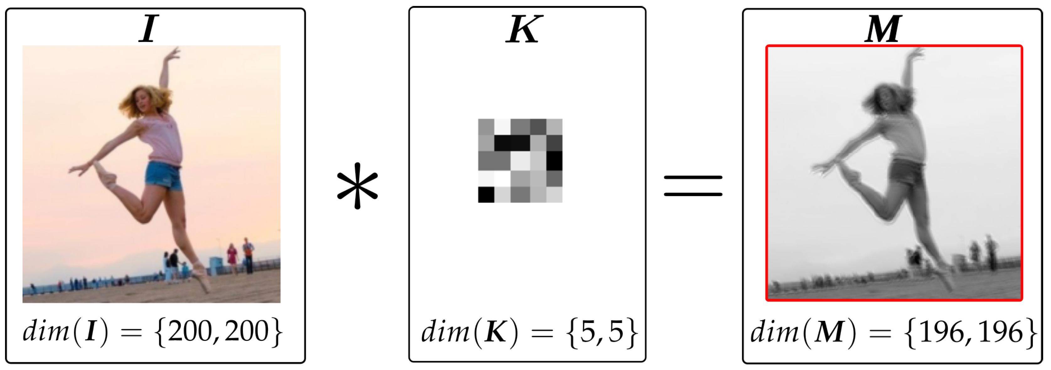
Convolutional networks are named as such because performing forward propagation in one of their layers l with sparse and tight weights implies calculating a convolution of the input  I R m × n  to layer l with at least one kernel  K R f × f  of a determined odd squared size f. The result of this convolution is a feature map  M  (Figure 4).
The reason for using an odd-sized kernel (such as  3 × 3  or  5 × 5 ) is because it provides a well-defined center element, allowing the filter to align symmetrically with the input at each position. Additionally, it make it possible to apply equal padding on all sides, preserving the spatial dimensions of the input in the resulting feature maps.
Assume a general function  d i m ( X )  that maps a matrix  X  to its dimensions. Then, the dimensions of the input, kernel, and feature map are as follows:
d i m ( I ) = def { m , n }
d i m ( K ) = def { f , f }
d i m ( M ) = { m f + 1 , n f + 1 } .
In deep learning, the term ’convolution’ usually refers to the mathematical operation of discrete cross-correlation, which is the operation implemented by most deep learning frameworks. Assuming an input map  I  and a kernel  K , one-based index cross-correlation takes the following form:
( I K ) ( i , j ) l = m n x i + m 1 , j + n 1 l 1 · w m , n l
z i , j l = ( I K ) l + b i , j l
a i , j l = z i , j l ,
where  b i , j l  is the bias of the pre-activation  z i , j l  and  a i , j l = z i , j l  for the  i , j  element of a  2 D  feature map.
Furthermore, the convolution operation can be generalized in a number of ways: first, the manner in which the kernel is slid over the input map. The kernel must not necessarily be moved to the next immediate spatial element to compute the Frobenious product. Instead, the kernel may be slid across a number s of spatial locations. This is called the stride s, and the corresponding operation may be called a strided convolution. The baseline convolution has  s = 1 .
Second, the kernel may be shifted beyond the elements at the border of the input map. Sliding the kernel such that it entirely lies within the input map has the advantage that all the elements of the feature map are a function of equal numbers of elements in the input. However, it also has the disadvantage of progressively reducing the output (Equation (56)) until the extreme stage where a  1 × 1  output can not be meaningfully further processed. Alternatively, the spatial dimensions may be preserved by zero-padding the input with p elements. When  p = 0  (no padding), the operation is called valid convolution, which is one of the most common. In contrast, constant spatial dimensionality across inputs and outputs may be achieved by performing the same convolution with the corresponding  p > 0  padding.
Finally, the convolution operation may be generalized to operate on multidimensional inputs, e.g., RGB images, producing multidimensional outputs. This generalized convolution is termed convolutions over volumes because the input, kernels, and output may be considered as having a width, height, and depth (also channel to avoid confusion with the network’s depth). This, in addition to the processing of batches (Section 5.5), results in CNNs usually operating in tensors of size  b × w × h × c , i.e., batch size b, two spatial dimensions of width w and height h, and c number of channels, respectively. In this tutorial, we focus on inputs (images) with a maximum of three channels. Without loss of generality, we will consider one instance batch  b = 1 ; therefore, we will omit the batch dimension. The input and the filters are required to have an equal number of channels c. The dimensions of the tensor of feature maps  M  are determined by the dimensions of the input, the size, and the number of kernels.
Regarding the dimensionality, convolving a multichannel input  I  with k multichannel kernels  K : , : , : , k  of equal dimensions results in a tensor of feature maps  M . The above function  d i m ( · )  can now be generalized to n dimensions. Assume a padding p and a stride s, then:
d i m ( I ) = def { w , h , c }
d i m ( K ) = def { f , f , c , k }
d i m ( M ) = { w 2 p f s + 1 , h 2 p f s + 1 , k } ,
where  x  is the floor function that rounds its argument to the nearest integer.
Correspondingly, the  2 D  convolution (Equation (57)) may be generalized to a  3 D  convolution in layer l, as expected. A specific element  M i , j , k  of a determined output channel k is calculated by (1) sliding the three-dimensional kernel  K : , : , : , k  with weights  w m , n , c  across the three-dimensional input, then (2) computing the tensor inner product  K : , : , : , k · A  of the kernel and the three-dimensional tensor  A  of overlapping input elements. Stacking the elements of all channels that have been generated by sliding k kernels produces the layer’s output volume  M l  with elements  M i , j , k l . That is:
( I K ) ( i , j , k ) l = c m n x i + m 1 , j + n 1 , c l 1 · w m , n , c , k l
z i , j , k l = ( I K ) ( i , j , k ) l + b l
M i , j , k l = z i , j , k l .

5.2. Pooling Layer

Yet another prominent method to reduce the amount of parameters in the network is to use a pooling layer. Pooling outputs the result of computing a determined summary statistic in neighborhoods of activations of the previous layer.
Like convolution, the pooling function may be viewed as sliding a multi-channel window over a multi-dimensional input with an equal amount of channels. Therefore, the pooling function may be considered as a filter of squared size f that may be shifted by a stride s, acting on a possibly p zero-padded input. Unlike the convolution layer, the pooling layer does not have weights that must be updated by the learning algorithm.
Additionally, pooling is applied to each channel independently. For an input volume  M  with dimensions  { w , h , c } , the pooling’s output  O  dimensionality is as follows:
d i m ( O ) = { w + 2 p f s + 1 , h + 2 p f s + 1 , c } .
While the pooling function may calculate several summary statistics on any combination of dimensions, the most used is the operator that yields the maximum among the corresponding channel input elements  M : , : , k  inside the sliding window  max ( X ) , termed max pooling. That is, in one-based index form,
O i , j , k l = max m max n M ( i · s 1 ) + ( m 1 ) , ( j · s 1 ) + ( n 1 ) , k l 1 .

5.3. ReLU Layer

As we mentioned, we adopted the simple layer terminology, where the non-linearities are not part of the convolutional layer. Instead, we consider that there is a ReLU layer that may be integrated into the network’s architecture. As expected, the ReLU layer computes Equation (21).

5.4. CNN Training

Forward and Back-Propagation in CNNs

Since CNNs are deep feedforward networks (Section 4), their weights may be initialized using the Kaiming method (Section 4.2.3). CNNs may also be trained with gradient descent (Section 3.4.2). In particular, forward propagation (Equations (63)–(65), (21) and (67)) must be performed to obtain the error at the output layer, followed by back-propagation.
As previously discussed (Section 4.2.3), while back-propagating the error, the derivatives of the loss function with respect to the parameters need to be computed in order to update the weights. For CNNs, we will follow the strategy that we described in Section 4.2.3. That is, (1) compute the error at the output layer, (2) computer the error of the current layer in terms of the next layer to be able to back-propagate, (3) compute the weight derivatives in terms of the error at the current layer, and (4) compute the derivative of the bias.
In a CNN, the convolutional layer’s parameters are the kernels’ weights and the layer biases; one for each kernel. Therefore, the goal of back-propagation may be restated as computing the derivatives of the loss with respect to the kernels and the bias. Additionally, the derivatives of the ReLU and max pooling layer must be considered.
Since now we are operating with 3D tensors, we define the derivative of the cost function with respect to one input element  z x , y , z l  as follows:
δ x , y , z l = J z x , y , z l .
Commonly, the output layer of a CNN is a dense layer. Therefore, the error at the output layer  δ  may be computed in the same manner as for a general ANN (Equation (39)). As we will see, the architecture of CNNs comprises ReLU and max pooling layers. Therefore, the computation of the backpropgation and concrete weights (Equations (47) and (51)) must be adapted to these layers.
Fortunately, neither the ReLU layer nor the max pooling layer contain weights that must be updated by SGD. This means that Equations (51)–(53) must be disregarded for these two layers. However, in our strategy, these layers must be able to transmit the error back to preceding layers, which indeed requires readjusting Equation (47) (backpropagation equation between layer  l + 1  and l). For that matter, we may consider that the errors at these layers are known, e.g., after having been back-propagated by a dense layer.
On order to adapt Equation (47) to the ReLU layer, note that because the layer does not contain weights, the weight matrix  W  vanishes. Also, we now consider the local gradient  δ i , j , k l  to be a tensor element. Since forward-propagating through a ReLU layer is conducted element-wise, the input and output dimensions are preserved, and so happens with back-propagation. This allows for equal indexing of the back-propagated error arriving at the layer and the calculated local gradient. That is,
δ i , j , k l = δ i , j , k l + 1 · g ( z i , j , k l ) ,
where,  g ( z i , j , k l )  is the derivative of the ReLU evaluated at the tensor element  M i , j , k l .
Conversely, one key observation is that the max pooling layer does change the dimensionality of its input. Specifically, it down-samples the input by discarding its activations in the sliding window, except for the one with the maximum value. These units, whose activations were discarded, will obviously receive zero gradient.
During forward propagation, the max pooling operation does more than just select the maximum value in each window; it also “memorizes” the indices of these maximum values within the tensor. This creates a one-to-one mapping between each pooled activation  M m , n , k —the maximum value in each region—and the corresponding output element  O i , j , k  based on these retained indices. When back-propagating, only the unit whose index has been memorized receives a non-zero gradient. This is called gradient routing, because the max pooling layer routes back the gradient it receives to the unit whose maximum value was selected. For example, if the maximum value in a pooling window is at  M 1 , 2 , 3 , and this value is mapped to an output element, say  O 0 , 1 , 3 , the index  { 1 , 2 , 3 }  is preserved. Consequently, during back-propagation, this memorized index ensures that the gradient flows back to and only to  M 1 , 2 , 3 .
Because the partial derivative of the max operation  g M m , n , k  with respect to the pooled value  M m , n , k  equals one, Equation (47) takes the following form:
δ m , n , k l = δ i , j , k l + 1 if M m , n , k = O i , j , k 0 otherwise .
Having obtained the backpropagation rules of the ReLU and max pooling layer, it remains to discussed back-propagation on the convolutional layer. Indeed, in this case, the kernel weights and the units bias must be updated. Consequently, (1) the back-propagation rule of the convolution layer and (2) the derivative of the loss function with respect to the kernel weights and neuron bias must be derived.
First, let us consider the backpropagation rule for the convolutional layer. Like for fully connected layers, we start by observing that the chain rule may be employed to compute the neuron error in layer l. Also, to unclutter the notation, we will assume zero padding and unit stride ( p = 0 s = 1 ).
Unlike the general case, one input element in a convolutional layer l affects one or more elements in layer  l + 1 , but not all. Therefore, the partial derivative of the cost function with respect to one element  z m , n , c l  must aggregate the partial derivatives of all elements  z · , · , · l + 1  affected by it.
Because the convolutional layer down-samples the input spatial dimensions, care must be taken when selecting the output element indices whose contributions must be added. One important observation is that one input element affects all feature maps (albeit not all elements); thus, we must sum over all output channels k. Another observation is that non-multi-channel kernel  K m , n , c  moves across the depth dimension; therefore, its index does not contain offsets. After having considered the channels, we must further consider the effect of the input element  z m , n , c l  in one specific output channel  z : , : , k l . Given a specific channel k, the input element affects a number of elements in that channel, namely the elements fixed at position  m , n  and that are the result of the kernel having been slit by by  a , b  (input perspective; we introduce auxiliary indices a and b). Finally, we know that all kernels have the same dimensionality (they are packed in one 4D-tensor); thus, we can use the same iterators  a , b  for all kernels. These observations lead to the following:
δ m , n , u l = k a b J z m a + 1 , n b + 1 , k l + 1 · z m a + 1 , n b + 1 , k l + 1 z m , n , u l
= k a b δ m a + 1 , n b + 1 , k l + 1 · z m a + 1 , n b + 1 , k l + 1 z m , n , u l .
In Equation (72), the neuron error  J z m a + 1 , n b + 1 , k l + 1  has been substituted by its definition  δ m a + 1 , n b + 1 , k l + 1 .
We now focus on the second term in the right and expand it. Here, again, we introduce auxiliary indices  p , q , r , and use  x · , · , · l = z · , · , · l  (as mentioned, we assumed we are operating on linear layers).
z m a + 1 , n b + 1 , k l + 1 z m , n , c l = z m , n , c l p q r z ( m a + 1 ) + p 1 , ( n b + 1 ) + q 1 , r l · w p , q , r , k l + 1 + b l
= z m , n , c l p q r z m a + p , n b + q , r l · w p , q , r , k l + 1 + b l
= z m , n , c l z m , n , c l · w a , b , c , k l + 1
= w a , b , c , k l + 1 .
In Equation (73), we expand as mentioned above, then in Equation (74), we reduce the indices as  ( m a + 1 ) + p 1 = m a + p , ( n b + 1 ) + q 1 = n b + q . In Equation (72), it all partial derivatives may be observd with respect to  z m , n , c l , except when  a = p , b = q , r = c . Accordingly, the weights must have indices  a , b , c , k . Then, plugging Equation (76) into Equation (72), we have the following:
δ m , n , c l = k a b δ m a + 1 , n b + 1 , k l + 1 · w a , b , c , k l + 1 .
δ m , n , c l = δ m , n , c l + 1 rot 180 ( w a , b , c , k l + 1 ) .
Equation (77) is a standard convolution of the error at the end of the convolutional layer (the error it receives from the following layer) with the kernel tensor. Equivalently, Equation (77) may expressed as a cross-correlation with a flipped kernel (Equation (78)) by rotating the 3D kernel  180  around the depth axis ( rot 180 ( · ) ). Note in Equation (77) that the matrix with elements  δ · , · , · l + 1  has reduced spatial dimensions compared with the input I to the convolutional layer. Therefore, to back-propagate, the matrix must be zero-padded (upsampled) by the amount  f p 1 = f 1  (recall that f is the filter size) after having been convolved, and I’s dimensions are obtained. In other words, backpropagation requires a transposed convolution. Furthermore, Equation (77) suggests that, in order to propagate the error to the input unit  δ m , n , c l , one must collect the kernel weights in the channel c of all kernels k and multiply them by the corresponding elements in the gradient tensor at the corresponding k feature map.
An interesting concrete example in given in [30]:
“In order to understand the transposition above, consider a situation in which we use 20 filters on the 3-channel RGB volume in order to create an output volume of depth 20. While backpropagating, we will need to take a gradient volume of depth 20 and transform to a gradient volume of depth 3. Therefore, we need to create 3 filters for backpropagation, each of which is for the red, green, and blue colors. We pull out the 20 spatial slices from the 20 filters that are applied to the red color, invert them (…), and then create a single 20-depth filter for backpropagating gradients with respect to the red slice. Similar approaches are used for the green and blue slices”.
Similarly, the derivative of the cost function with respect to to the kernel weights  w · , · , · l  must be computed. A kernel weight  w m , n , c , k l  affects only the elements in the k feature map. Therefore, when applying the chain rule, its gradient must add the partial derivative of all these elements:
J w m , n , c , k l = i j J z i , j , k l · z i , j , k l w m , n , c , k l
= i j δ i , j , k l · z i , j , k l w m , n , c , k l .
The same techniques as before may be applied to Equation (79), i.e., substitute the neuron error with its definition, which results in Equation (80). Then, the second term in the right may be expanded as follows:
z i , j , k l w m , n , c , k l = w m , n , c , k l r p q z i + p 1 , j + q 1 , r l · w p , q , r , k l + b l
= ( z i + m 1 , j + n 1 , c l · w m , n , c , k l ) w m , n , c , k l
= z i + m 1 , j + n 1 , c l 1 .
Calculating the partial derivative of the triple summation in Equation (81) reduces all terms to zero, except the term with index  p = m q = n , and  r = c . The result (83) may be substitute into Equation (80), i.e.,
J w m , n , c , k l = i j δ i , j , k l · z i + m 1 , j + n 1 , c l 1
Comparing Equation (82) with Equation (78), it may be noted that while back-propagating the error, both the kernel and the layer error must be rotated.
The derivation of the error of the cost function with respect to the bias also follows the above strategy. The shared bias affects all activations in the feature map. However, based on Equation (57), we may conclude that the partial derivative of all activations  i , j , k  with respect to the bias equal one, i.e.,  z i , j , k l b l = 1 . Thus,
J b l = k a b J z a , b , k l · z a , b , k l b l
= k a b δ a , b , k l .

5.5. Batch Normalization

One of the earliest findings in machine learning was that inputting features in different scales hinders ANN learning [31,32]. Except for settings where preprocessing of the features is not desired, feature normalization is standard practice.
While features are supplied to the ANN at the input layer, the question arises naturally whether the same strategy may be applied to the hidden layers. As shown by Equation (22), a determined hidden layer’s input is a highly non-linear function of the ANN inputs. From the perspective of the hidden layer, the input to its units constantly varies in possibly several scales, complicating learning.
This motivates the batch normalization (also Batchnorm) method [33]. Batchnorm proposes to normalize the input to a layer to stabilize optimization. This method may be presented in several forms (see [2,33]). Specifically, while the former explains Batchnorm from a transform perspective, the latter considers it a re-parameterizing technique: “Batch normalization provides an elegant way of reparametrizing almost any deep network”. Here, we follow this approach.
Consider a mini-batch of activations (output) at a determined layer  l 1 , which may be normalized to train the layer l faster. This may be represented by a design matrix  H R n × m  with elements  a i j , where i is the activation of unit i corresponding to one mini-batch example  x ( j ) . That is, the rows of  H  are the activation vectors corresponding to one training example, while the columns are the activations at unit i of all mini-batch training examples.
Batchnorm normalizes each activation independently by subtracting the mean  μ  and dividing it by the standard deviation  σ  on a per-column basis. That is,
μ j = 1 m i = 1 m a i j
σ j = δ + 1 m i = 1 m | a i j μ j | 2
μ = { μ 1 , , μ m }
σ = { σ 1 , , σ m }
H = H μ σ ,
where the components of the mean vector  μ  (Equation (89)) and the standard deviation vector  σ  (Equation (90)) are the mean (Equation (87)) and the standard deviation (Equation (88)) of each unit. In Equation (88), a small constant  δ  (e.g.,  10 8 ) is added for numerical stability. In Equation (91), the vectors  μ  and  σ  are broadcasted to normalize  a i j  using  σ j  and  μ j .
Although intuitive, restricting the distribution of the activation to have zero mean and unit standard deviation is an arbitrary choice. A priori, it is not guaranteed that this setting will result in accelerating learning. Optimally, the ANN should learn how to transform the activations.
Indeed, instead of replacing  H  by its normalized form  H , the activations may be replaced with the parametrized form  B N ( H ) = γ H + β , where the vectors  γ  and  β  may be learned by SGD, say. The arithmetic here is as described above, i.e., the activation  a i j  is replaced by
γ j · a i j μ j δ j + β j .
This form has the advantage that it can recover the original normalized activations  H  for  γ = 1 , β = 0 , and, more importantly it allows for the activation distribution to be arbitrarily shifted and scaled by the learning algorithm.
During training, the learning algorithm updates the parameters  β  and  δ  so that when training has finished, these parameters are ready to use for inference. In contrast, the empirical statistics  μ  and  δ  used to normalize the activations are computed on a mini-batch (Equations (87) and (88)). This may pose two problems. First, during inference with one instance, the statistics are not well defined (because of the unit batch size). Second, if inference is conducted for a mini-batch, the relation of one determined instance with respect to its predicted target is not deterministic because the statistics depend on the batch in which this instance may appear.
One standard solution (that we also use) is to maintain running averages of the statistics during training, i.e., for each activation,  μ  and  σ  are averaged over all mini-batches in the training set. Then, inference is conducted with these fixed statistics.
The effects of Batchnorm are to some extent controversial in the scientific community. For example, while the authors of the original paper claimed that Batchnorm diminishes the constant variation of the mean and variance of the hidden layers (internal covariance shift) [33], other scientists have shown that Batchnorm’s efficiency is based on a different mechanism [34]. That being said, Batchnorm is an indispensable part of ANNs.

6. Summary

In this tutorial, we examined the foundations of deep learning with special focus on convolutional neural networks. Deep learning belongs to a wider set of methods called machine learning, with the main goal of developing systems or agents that are able to learn from data.
The most important concept of learning is generalization; that is, given a dataset, the learning algorithm is trained on the data to perform a specific task and is required to accomplish the task on data it did not experience before. In particular, it is expected that the agent outputs a certain type of inference or prediction based on the data. Common tasks are classification (predicting a category) and regression (predicting a continuous quantity); for example, classifying images of cars and regressing the height of a person in a picture.
The dataset is a key component of the learning algorithm. It is composed of examples or observations, each having features that contain useful information for training the agent. The dataset may include a prediction target for every example, such that the agent can learn by processing the examples and observing the correct prediction it has to output. This is called supervised learning, and the targets accompanying the examples are the ground truth. The opposite case, in which the dataset does not contain the ground truth, is called unsupervised learning. Additionally, there are other two forms of learning, namely semi-supervised learning and reinforcement leaning, but this tutorial is focused on supervised learning.
Deep learning borrows concepts from learning theory; therefore, it assumes that there is a function in a hypothesis space that maps the examples to their targets. In this view, the learning agent is the model that approximates the function in the hypothesis space. The lower the generalization error, the better the approximation. Theoretically, the dataset may be divided into a training set, where the training error may be calculated, and a test set, where generalization error is assessed. However, while training, the agent has no access to the test set and can only estimate the generalization error using the training set. This error is called empirical risk; therefore, the agent general strategy from the perspective of leaning theory is termed empirical risk minimization.
In addition to learning theory, deep learning also borrows concepts from statistics and probability theory. In particular, the leaning agent is considered an estimator that may be parameterized. When analyzing ANNs, these parameters are conceptualized as weights. This leads to the conclusion that the estimator function is the neural network.
Artificial neural networks are comprised of artificial neurons. The neurons compute a non-linear function of the linear combination of the inputs.
To train the network, gradient descent may be used. Gradient descent requires updating the network weights. In order to compute the suitable update magnitude, three steps must be iteratively conducted. First, the information is forward-propagated from the input layer, through the neurons, and to the output layer. Second, the error of the cost function is calculated with respect to the parameters at the output layer, and finally, the error is back-propagated to the input layer.
Most of the fundamental principles on which DL rests have been developed decades ago; for example, statistical learning, learning theory, SGD, Perceptron, Backprop, and CNNs. However they continue to be used in all modern DL applications.
Several of the most important innovations in DL were inspired by the structure and function of human and animal brains, including Perceptron, ReLU, receptive fields (CNNs), and BatchNorm.
Although regression tasks may be cast to classification tasks by discretizing the output, regression has a number of advantages compared to classification when the task involves predicting continuous quantities. For example, regression provides higher resolution, less information loss, or, depending on the manner in which the problem is framed, more appropriate error metrics. In cases like weather prediction (temperature and future rainfall), regression is optimal.
While regression offers precise predictions and is suitable for continuous data, it comes with challenges such as sensitivity to outliers, complexity in evaluating performance, and difficulty in handling nonlinear relationships or imbalanced data. For some problems, these factors can make classification a more straightforward or effective approach.
That being said, deep regression is a powerful framework that can be employed to tackle several problems in the real world.

Author Contributions

Y.G.T. took the lead in writing the manuscript and designing the figures. H.A.M. performed critical revisions and ensured the accuracy of the manuscript. Both Y.G.T. and H.A.M. contributed to and approved the final version of the manuscript. H.A.M. supervised the project. All authors have read and agreed to the published version of the manuscript.

Funding

No funding was provided.

Data Availability Statement

Not applicable.

Conflicts of Interest

The authors declare no conflict of interest.

Notation

In this tutorial, we use the following notation:
Number and Arrays
aA scalar (integer or real)
a A vector
A A matrix
A A tensor
aA scalar random variable
a A vector-value random variable
A A matrix-value random variable
Sets
A A set
R The set of real numbers
{ 0 , 1 , , n } The set of all integers between 0 and n
Indexing
a i Element i of vector  a
a i All elements of vector  a  except for element i
A i , j Element  i , j  of matrix A
A i , : Row i of matrix  A
A : , i Column i of matrix  A
A i , j , k Element  ( i , j , k )  of a tensor A
A : , : , i 2D slice of a 3D tensor
A : , : , : , i 3D slice of a 4D tensor
Linear Algebra Operations
A T Transpose of matrix  A
A B Element-wise (Hadamard) product of A  and  B
Calculus
d y d x Derivative of y with respect to x
z y Partial derivative of y with respect to x
x y Gradient of y with respect to x
Probability and Information Theory
P ( a ) A probability distribution over a discrete variable
p ( a ) A probability distribution over a continuous variable,
or over a variable whose type has not been defined
a P Random variable a with distribution P
E x P [ f ( x ) ]  or  E f ( x ) Expectation of  f ( x )  with respect to  P ( x )
D K L ( P Q ) Kullback–Leibler divergence of P and Q
N ( x ; μ , Σ ) Gaussian distribution over  x  with mean  μ  and covariance  Σ
Functions
f : A B Function f with domain A  and range  B
f ( · ) ( i ) function i of an ordered set of functions
f g Composition of functions f and g
f ( x ; θ ) A function of x  parametrized by  θ
log x Natural logarithm of x
σ ( x ) Logistic sigmoid,  1 1 + exp ( z )
ζ ( x ) Softplus,  log ( 1 + exp ( z ) )
x p L p  norm of  x
x L 2  norm of  x
Datasets and Distributions
p d a t a The data-generating distribution
p ^ d a t a The empirical distribution defined by the training set
X A set of training examples
x ( i ) The i-th example (input) from a dataset
y i y ( i ) , or  y ( i ) The target associated with  x ( i )  for supervised learning
X The  m × n  matrix with input example x ( i )  in row  X i , :

References

  1. Rusell, S.J.; Norvig, P. Artificial Intelligence. A Modern Approach; Pearson Education, Inc.: Upper Saddle River, NJ, USA, 2010. [Google Scholar]
  2. Goodfellow, I.; Bengio, Y.; Courville, A. Deep Learning; MIT Press: Cambridge, MA, USA, 2016. [Google Scholar]
  3. Shalev-Shwartz, S.; Ben-David, S. Understanding Machine Learning; Cambridge University Press: Cambridge, UK, 2014. [Google Scholar]
  4. Hastie, T.; Tibshirani, R.; Friedman, J. The Elements of Statistical Learning: Data Mining, Inference and Prediction, 2nd ed.; Springer: Berlin/Heidelberg, Germany, 2009. [Google Scholar]
  5. McElreath, R. Statistical Rethinking: A Bayesian Course with Examples in R and Stan; Chapman and Hall/CRC: Boca Raton, FL, USA, 2020. [Google Scholar]
  6. Krogh, A.; Hertz, J. A Simple Weight Decay Can Improve Generalization. In Proceedings of the Advances in Neural Information Processing Systems, Denver, CO, USA, 2–5 December 1991; Moody, J., Hanson, S., Lippmann, R., Eds.; Morgan-Kaufmann: Burlington, MA, USA, 1991; Volume 4. [Google Scholar]
  7. McCulloch, W.S.; Pitts, W. A logical calculus of the ideas immanent in nervous activity. Bull. Math. Biophys. 1943, 5, 115–133. [Google Scholar] [CrossRef]
  8. Hebb, D.O. The Organization of Behavior: A Neuropsychological Theory; Psychology Press: London, UK, 1949. [Google Scholar]
  9. Rosenblatt, F. The Perceptron—A Perceiving and Recognizing Automaton; Technical Report 85-460-1; Cornell Aeronautical Laboratory: Ithaca, NY, USA, 1957. [Google Scholar]
  10. Jarrett, K.; Kavukcuoglu, K.; Ranzato, M.; LeCun, Y. What is the best multi-stage architecture for object recognition? In Proceedings of the 2009 IEEE 12th International Conference on Computer Vision, Kyoto, Japan, 29 September–2 October 2009; pp. 2146–2153. [Google Scholar]
  11. Minsky, M.; Papert, S. Perceptrons: An Introduction to Computational Geometry; MIT Press: Cambridge, MA, USA, 1969. [Google Scholar]
  12. Lu, Z.; Pu, H.; Wang, F.; Hu, Z.; Wang, L. The Expressive Power of Neural Networks: A View from the Width. Adv. Neural Inf. Process. Syst. 2017, 30, 6232–6240. [Google Scholar]
  13. Cybenko, G. Approximation by superpositions of a sigmoidal function. Math. Control. Signals Syst. 1989, 2, 303–314. [Google Scholar] [CrossRef]
  14. Gripenberg, G. Approximation by neural networks with a bounded number of nodes at each level. J. Approx. Theory 2003, 122, 260–266. [Google Scholar] [CrossRef]
  15. Maiorov, V.; Pinkus, A. Lower bounds for approximation by MLP neural networks. Neurocomputing 1999, 25, 81–91. [Google Scholar] [CrossRef]
  16. Hardt, M.; Recht, B.; Singer, Y. Train faster, generalize better: Stability of stochastic gradient descent. In Proceedings of the the 33rd International Conference on Machine Learning, New York, NY, USA, 20–22 June 2016; Balcan, M.F., Weinberger, K.Q., Eds.; Proceedings of Machine Learning Research. Volume 48, pp. 1225–1234. [Google Scholar]
  17. Robbins, H.E. A Stochastic Approximation Method. Ann. Math. Stat. 1951, 22, 400–407. [Google Scholar] [CrossRef]
  18. Newton, D.; Yousefian, F.; Pasupathy, R. Stochastic Gradient Descent: Recent Trends. In Recent Advances in Optimization and Modeling of Contemporary Problems; INFORMS: Catonsville, MD, USA, 2018; pp. 193–220. [Google Scholar] [CrossRef]
  19. Goh, G. Why Momentum Really Works. Distill 2017, 2, e6. [Google Scholar] [CrossRef]
  20. Bishop, C.M. Pattern Recognition and Machine Learning (Information Science and Statistics), 1st ed.; Springer: Berlin/Heidelberg, Germany, 2007. [Google Scholar]
  21. Nielsen, M.A. Neural Networks and Deep Learning; Springer: Cham, Switzerland, 2015. [Google Scholar]
  22. He, K.; Zhang, X.; Ren, S.; Sun, J. Delving Deep into Rectifiers: Surpassing Human-Level Performance on ImageNet Classification. In Proceedings of the 2015 IEEE International Conference on Computer Vision (ICCV), Santiago, Chile, 7–13 December 2015; pp. 1026–1034. [Google Scholar] [CrossRef]
  23. Glorot, X.; Bengio, Y. Understanding the difficulty of training deep feedforward neural networks. In Proceedings of the Thirteenth International Conference on Artificial Intelligence and Statistics, Sardinia, Italy, 13–15 May 2010; Teh, Y.W., Titterington, M., Eds.; Chia Laguna Resort: Sardinia, Italy, 2010. Proceedings of Machine Learning Research. Volume 9, pp. 249–256. [Google Scholar]
  24. Paszke, A.; Gross, S.; Massa, F.; Lerer, A.; Bradbury, J.; Chanan, G.; Killeen, T.; Lin, Z.; Gimelshein, N.; Antiga, L.; et al. PyTorch: An Imperative Style, High-Performance Deep Learning Library. In Advances in Neural Information Processing Systems 32; Wallach, H., Larochelle, H., Beygelzimer, A., d’Alché-Buc, F., Fox, E., Garnett, R., Eds.; Curran Associates, Inc.: San Francisco, CA, USA, 2019; pp. 8024–8035. [Google Scholar]
  25. Hutter, F.; Kotthoff, L.; Vanschoren, J. (Eds.) Automated Machine Learning—Methods, Systems, Challenges; Springer: Berlin/Heidelberg, Germany, 2019. [Google Scholar]
  26. Fukushima, K. Neocognitron: A self-organizing neural network model for a mechanism of pattern recognition unaffected by shift in position. Biol. Cybern. 1980, 36, 193–202. [Google Scholar] [CrossRef] [PubMed]
  27. González Tejeda, Y.; Mayer, H.A. A Neural Anthropometer Learning from Body Dimensions Computed on Human 3D Meshes. In Proceedings of the 2021 IEEE Symposium Series on Computational Intelligence (SSCI), Virtual, 5–7 December 2021; pp. 1–8. [Google Scholar] [CrossRef]
  28. Krizhevsky, A.; Sutskever, I.; Hinton, G.E. Imagenet classification with deep convolutional neural networks. Adv. Neural Inf. Process. Syst. 2012, 25, 1097–1105. [Google Scholar] [CrossRef]
  29. Simonyan, K.; Zisserman, A. Very deep convolutional networks for large-scale image recognition. arXiv 2014, arXiv:1409.1556. [Google Scholar]
  30. Aggarwal, C.C. Neural Networks and Deep Learning. A Text book.; Springer International Publishing: Berlin/Heidelberg, Germany, 2018. [Google Scholar] [CrossRef]
  31. Bishop, C. Neural Networks for Pattern Recognition; Oxford University Press: Oxford, UK, 1995. [Google Scholar]
  32. LeCun, Y.A.; Bottou, L.; Orr, G.B.; Müller, K.R. Efficient BackProp. In Neural Networks: Tricks of the Trade; Lecture Notes in Computer Science; Springer: Berlin/Heidelberg, Germany, 2012; pp. 9–48. [Google Scholar] [CrossRef]
  33. Ioffe, S.; Szegedy, C. Batch Normalization: Accelerating Deep Network Training by Reducing Internal Covariate Shift. In Proceedings of the 32nd International Conference on Machine Learning, Lille, France, 7–9 July 2015; Bach, F., Blei, D., Eds.; Proceedings of Machine Learning Research. Volume 37, pp. 448–456. [Google Scholar]
  34. Santurkar, S.; Tsipras, D.; Ilyas, A.; Madry, A. How Does Batch Normalization Help Optimization? In Proceedings of the Advances in Neural Information Processing Systems, Montréal, QC, Canada, 3–8 December 2018; Bengio, S., Wallach, H., Larochelle, H., Grauman, K., Cesa-Bianchi, N., Garnett, R., Eds.; Curran Associates, Inc.: San Francisco, CA, USA, 2018; Volume 31. [Google Scholar]
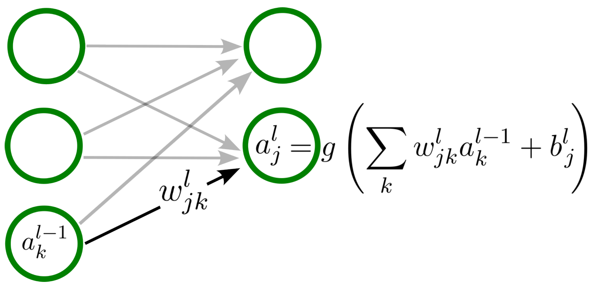
Figure 1. ANN weight notations illustrated. The figure depicts two fully connected hidden layers of an arbitrary ANN. Layer l (right) has two neurons (green circles), and the preceding layer  l 1  (left) has three units. TNeuron j is the second unit (from top to bottom) in layer l; the third unit k in layer  l 1  has activation  a k l 1 . Among all the connections (mostly in gray), we emphasize (in black) the connection from unit k in layer  l 1  to unit j in layer l; the weight of this connection is denoted as  w j k l . Supposing the right layer is the second hidden layer, then the depicted weight is concretely  w 23 2 . To calculate the activation  a j l  of this neuron j, the weights of all incoming connections from all neurons  { w j 1 l , w j 2 l , , w j k l }  in layer  l 1  must be multiplied by the corresponding activation  { a 1 l 1 , a 2 l 1 , , a k l 1 } . The bias  b j l  must be added to the resulting summation, and the activation function  g ( · )  must be applied element-wise. To avoid having to transpose the weight matrix representing all connections at one layer ( ( W l ) T ), the index order in the weights is set to be  j k .
Make 06 00132 g001
Figure 2. An example of a CNN architecture performing regression. Here, we show an adapted version of our neural anthropometer from [27]: a CNN that is able to regress eight human body dimensions like height or waist circumference from synthetic images of persons in two poses (top left). The inputs to the network are grayscale  200 × 200  pixel synthetic images of 3D real human meshes (top middle). The supervision signal is a vector of eight human body dimensions (top right), and the loss  L MSE  (bottom right) is the Mean Square Error (MSE) (Equation (14)) between the actual and the estimated measurements. Hyperparameters for learning with this CNN are set as described in Table 1. We discuss the details of the layer types in Section 5.1, Section 5.2 and Section 5.3. At the bottom, the five gray rectangular cuboids represent the input and the feature maps. The red and green horizontal pyramids represent the convolution (Section 5.1) and max pooling (Section 5.2) layers, respectively. The black grids are rectified linear unit (ReLU) layers (Section 5.3), and the connected circles are fully connected layers (Section 4.1.2). In this case, (1) the first convolutional layer applies a convolution with a 5-pixel square kernel to produce a feature map of size  196 × 196 × 8 . The tensor is then passed through a ReLU, and batch normalization (Section 5.5, not shown here) is applied. Next, (2) max pooling with stride 2 is used, producing a tensor of size  98 × 98 × 8 . Then, (3) the tensor is sent to a second convolutional layer with a 5-pixel square kernel and 16 output channels, resulting in a tensor of size  94 × 94 × 16 . Next, (4) pooling is applied as before, producing a tensor of size  47 × 47 × 16 , and (5) the output is flattened to a tensor of size 35,344. This tensor is passed to a fully connected layer and again through a ReLU (not shown). The output layer (6) regresses the eight human body dimensions in meters. Using the simple layer terminology, the depth of this network is 10: convolution + ReLU + Batchnorm + max pooling + convolution + ReLU + max pooling + fully connected + ReLU + fully connected (output layer). Other common counting schema include only the layers with learnable parameters, in which case this network would have a depth of 5.
Make 06 00132 g002
Figure 3. Possible input and first hidden layer of a hypothetical CNN. Left: A general ANN that receives the input  { x 1 , , x 9 } . The first hidden layer l contains four neurons with activation  { a 1 , , a 4 }  (circles in orange, magenta, green, and red colors, from top to bottom). We emphasize the first two neurons and their connections to the input layer. Note that the neurons are not fully connected to the input layer, e.g., the unit  a 1 l  is connected to inputs  { x 1 , x 2 , x 4 , x 5 } , which form its receptive field, but not to input  x 3 . Moreover, all four neurons have equal weights  { w 1 , , w 4 } , indicated by the four arrows arriving to the units. Right: The same network seen as a CNN. The input, the weights, and the neurons have a grid structure. The connections of the neurons to the input induce a  2 D  convolution  ( I K ) ( i , j )  of the input I ( 3 × 3  grid) with kernel K ( 2 × 2  grid). The convolution may be visualized as sliding the kernel over the input grid to produced a feature map, where every element of the feature map is the Frobenius product  K , A F  of the matrix defined by the kernel K and the overlapped input elements A, plus one shared bias. We highlight the computation of two elements of the feature map (the other two are not depicted) by the corresponding broken ( ) and broken with point ( · · ) arrows of the highlighted orange and magenta neurons, respectively. For example, the unit  a 1 , 1 l  has pre-activation  z 1 , 1 l = x 1 , 1 l · w 1 , 1 l 1 + + x 2 , 2 l · w 2 , 2 l 1 + b l . Note that there is only one bias  b l  per feature map. We adopt the simple layer terminology, where  a i , j l  is a linear unit that outputs a pre-activation  z i , j l . Therefore,  a i , j l = z i , j l . Supposing that the input I is an image, it may be observed that the sparse connections and the shared weights confer the network with the capability of establishing spatial relations among neighbor pixels. For an input of size  n × n  convolved with a  f × f  kernel, the size of the feature map is  n f + 1 × n f + 1 .
Make 06 00132 g003
Figure 4. From left to right, the rectangles represent the concepts of the input  I  being convolved with a filter  F  and the resulting feature map  M  of a CNN ( I F = M ). In order to exemplify these concepts, we modified our neural anthropometer network [27], which originally accepts as input a grayscale image, to accept an RGB image of  d i m ( I ) = { 200 , 200 }  (left). On the bottom of the rectangles, we indicate the dimensions of the corresponding tensor, as defined by the function  d i m ( X )  (Equations (54)–(56)). We display the first filter with  d i m ( F ) = { 5 , 5 }  of the first convolutional layer in the trained network. Note that, in order to enhance the visibility, we significantly scale the filter in the middle. On the right, the red border indicates the reduced dimensionality of  { 4 , 4 }  of the feature map with  d i m ( M ) = { 196 , 196 }  with respect to the input.
Make 06 00132 g004
Table 1. Hyperparameters. The table summarizes the hyperparameters that we use in this tutorial (first column). The second column indicates the corresponding interpretation. Furthermore, we specify the subsection in which they are described (third column), with their typical values in the fourth column.
HyperparameterInterpretationSectionDefault or Common Values
ϵ Learning rateSection 3.4.2 0.01 0.1
α Regularization coefficientSection 3.4.3 0.2
χ Number of epochsSection 4.2.15, 10, 100
nBatch size (SGD)Section 4.2.1100
υ MomentumSection 4.2.2 0.9
Disclaimer/Publisher’s Note: The statements, opinions and data contained in all publications are solely those of the individual author(s) and contributor(s) and not of MDPI and/or the editor(s). MDPI and/or the editor(s) disclaim responsibility for any injury to people or property resulting from any ideas, methods, instructions or products referred to in the content.