Article

Predictive Approach to the Phase Behavior of Polymer–Water–Surfactant–Electrolyte Systems Using a Pseudosolvent Concept

by
Ji-Zen Sheu
1 and
Ramanathan Nagarajan
1,2,*
1
Department of Chemical Engineering, The Pennsylvania State University, University Park, PA 16802, USA
2
US Army Combat Capabilities Development Command Soldier Center, Natick, MA 01760, USA
*
Author to whom correspondence should be addressed.
Colloids Interfaces 2024, 8(4), 40; https://doi.org/10.3390/colloids8040040
Submission received: 15 May 2024 / Revised: 17 June 2024 / Accepted: 19 June 2024 / Published: 21 June 2024
(This article belongs to the Special Issue Surfactants and Interfaces)

Abstract

:
A predictive approach to the phase behavior of four-component polymer–water–surfactant–electrolyte systems is formulated by viewing the four-component system as a binary polymer–pseudosolvent system, with the pseudosolvent representing water, surfactant, and the electrolyte. The phase stability of this binary system is examined using the framework of the lattice fluid model of Sanchez and Lacombe. In the lattice fluid model, a pure component is represented by three equation-of-state parameters: the hard-core volume of a lattice site ( v * ), the number of lattice sites occupied by the component (r), and its characteristic energy ( ε * ). We introduce the extra-thermodynamic postulate that r and v * for the pseudosolvent are the same as for water and all surfactant–electrolyte composition-dependent characteristics of the pseudosolvent can be represented solely through its characteristic energy parameter. The key implication of the postulate is that the phase behavior of polymer–pseudosolvent systems will be identical for all pseudosolvents with equal values of characteristic energy, despite their varying real compositions. Based on the pseudosolvent model, illustrative phase diagrams have been computed for several four-component systems containing alkyl sulfonate/sulfate surfactants, electrolytes, and anionic or nonionic polymers. The pseudosolvent model is shown to describe all important trends in experimentally observed phase behavior pertaining to polymer and surfactant molecular characteristics. Most importantly, the pseudosolvent model allows one to construct a priori phase diagrams for any polymer–surfactant–electrolyte system, knowing just one experimental composition data for a system at the phase boundary, using available thermodynamic data on surfactants and electrolytes and without requiring any information on the polymer.

Graphical Abstract

1. Introduction

The interaction between surfactants and polymers is an important phenomenon relevant to several practical applications in paints and coatings, personal care products, and the chemical, pharmaceutical, mineral processing, and petroleum industries [1,2,3,4,5,6]. The simultaneous presence of polymer and surfactant molecules alters the rheological properties of solutions, adsorption characteristics at solid–liquid interfaces, stability of colloidal dispersions, solubilization capacities in water for sparingly soluble molecules, and liquid–liquid interfacial tensions, and thereby impacts either beneficially or adversely the practical applications. An important application that has occupied the attention of researchers over the last five decades is the enhanced recovery of petroleum from existing reservoirs by chemical flooding [2,3,4,5]. In the chemical flooding process for enhanced oil recovery (EOR), a surfactant slug (often composed of anionic petroleum sulfonates) is injected into the ground to displace the formation oil. It is followed by a (typically anionic or nonionic) polymer-thickened mobility buffer and drive water. The surfactant slug is designed to generate ultra-low interfacial tensions against the formation oil. The polymer buffer is designed to possess adequate mobility control characteristics. The simultaneous presence of polymer and surfactant molecules in the reservoir results in interactions between these molecules, as well as with the minerals in the reservoir rocks. These interactions among polymer, surfactant, and electrolytes can drastically alter the properties of the surfactant slug and/or of the polymer mobility buffer from their designed characteristics, specifically due to changes in their phase behavior, leading to significant reduction in the anticipated oil recovery.
Many experimental studies on the phase behavior of solutions containing anionic or nonionic polymer molecules and anionic surfactant molecules have been carried out as part of the EOR research, in the laboratory as well as in large-scale oilfield reservoirs, since the early 1970s, but no theoretical treatment has been developed to date. The earliest experimental work is that of Trushenski et al. [7,8], who studied the phase behavior of solutions containing Mahogony AA sulfonate (a petroleum-derived surfactant), isopropyl alcohol, water, sodium chloride, and one of two polymers, Pusher 700 (a hydrolyzed polyacrylamide) or Xanflood (a Xanthan biopolymer). They found that the phase behavior of the systems differed very little for the two polymers. The phase behavior was not affected by polymer concentrations over the range of 500 to 1500 ppm. Szabo [9] examined systems composed of polymers, including Xanflood; hydroxyethyl and methyl celluloses; hydrolyzed and unhydrolyzed polyacrylamide; and polyacrylamido-methyl propane-sulfonate, as well as four different petroleum sulfonate-type surfactants. In all cases, phase separation into two liquid phases occurred on contact with the different components. The top phase was found to contain most of the polymer, while the bottom phase contained most of the sulfonate. As the polymer concentration was increased, the volume fraction of the surfactant-rich bottom phase decreased. The polymer concentration in the top phase and the sulfonate concentration in the bottom phase both increased. However, the polymer concentration in the bottom phase and the sulfonate concentration in the top phase remained constant. No systematic differences were seen with the variation in the type of polymer molecules.
Pope et al. [10] studied the effect of salt concentration on the phase behavior of polymer–surfactant solutions. The amount of NaCl required to induce phase separation in polymer–surfactant solutions was measured for combinations of different polymers and surfactants and at various concentrations of the two in solution. The electrolyte concentration at which phase separation occurs, designated as the critical electrolyte concentration (CEC), was found to be independent of the polymer type and polymer concentration (over the range 100 to 1000 ppm). No variation of CEC with the molecular weight of the polymer (over the range 4 × 10⁵ to 5 × 10⁶) was observed for polyethylene oxide.
Gupta [11] examined the effect of calcium salts on the phase behavior of a Pusher 700–Mahogony AA sulfonate solution containing 1600 ppm of the polymer. At 50 ppm concentration of calcium salt the solution was stable, whereas at 300 ppm the solution separated into a polymer-rich top phase and a surfactant-rich bottom phase. In general, the influence of the divalent electrolyte was more severe as to the phase stability compared to that of the monovalent electrolyte.
Kalpakci [12] investigated the phase behavior of several anionic and nonionic surfactant solutions in the presence of polymers. He found that the phase stability of the solutions decreased with the increasing concentration of the surfactant and of the electrolyte, as well as with increasing equivalent weight of the surfactant. The polymer size in the molecular weight range from 7 × 10⁴ to 2 × 10⁶ and polymer concentrations between 100 and 1500 ppm were found to have very little effect on the stability of the anionic sulfonate–polymer solutions. Further, unstable polymer–surfactant solutions were stabilized if the solution was subjected to ultrasonication, resulting in the breakdown of the molecular size of the polymer.
These experimental results in the early EOR literature show that phase separation is a common phenomenon in polymer–surfactant solutions in the presence of electrolytes, even with low concentrations of various components. The phase separation patterns are not significantly influenced by the molecular type or the molecular size of the polymer for the high molecular-weight polymers studied or by variations in polymer concentrations over the limited range of 100 to 1500 ppm typically investigated for EOR applications. The phase behavior is, however, critically affected by the equivalent weight of the surfactant and by the type and amount of the electrolyte added. The stability of the polymer–surfactant solution is enhanced if the polymer’s molecular weight is significantly reduced. Beyond these generalizations, little is known concerning the phase behavior of polymer–surfactant solutions from a predictive point of view, even after forty years of EOR research. Recent oil field simulations [3,4,5] have highlighted the need for reliable information on polymer–surfactant phase behavior, if realistic predictions of oil recovery efficiencies are to be made. Addressing this long-unfulfilled need is the motivation for this work.
The principal goal of this work is to develop a predictive approach to the phase behavior of aqueous solutions containing polymer, surfactant, and electrolyte molecules. Towards this goal, we postulate a novel approach to treat the four-component system of polymer, surfactant, electrolyte, and water by viewing it as a pseudo-binary system. The essence of this approach is as follows. One component of the pseudo-binary system is the polymer molecule, treated as the solute molecule. The other component, termed here the pseudosolvent, is made up of water, the surfactant, and the electrolyte. The thermodynamics of this solute–pseudosolvent binary system are quantitatively described using the formalism of any suitable polymer solution theory available in the literature. The criterion of phase separation stipulated by the polymer solution theory is then applied to the pseudo-binary system in order to find the composition boundary of the pseudo-components at which the solution undergoes phase separation. This composition boundary is then reinterpreted in terms of the actual concentrations of the surfactant and the electrolyte constituting the pseudosolvent. The predictions of the treatment are then compared to experimental results obtained on some polymers and surfactants of the type relevant to EOR.
In Section 2, the experimental methods and the materials used, and the observed phase behavior of some polymer and surfactant systems of interest to the enhanced oil recovery application, are briefly described. In Section 3, the conceptual outline of the pseudosolvent model is presented. The pseudosolvent model is quantitatively developed in Section 4, and the estimation of the model parameters is explained in detail. Phase diagrams are computed and compared to the experimentally measured ones in Section 5. Most importantly, for ease of practical applications, a simple approach to constructing phase diagrams using one experimentally measured surfactant–electrolyte composition lying at the phase boundary is proposed, without requiring any information on the polymer. The last section summarizes the principal conclusions from this work.

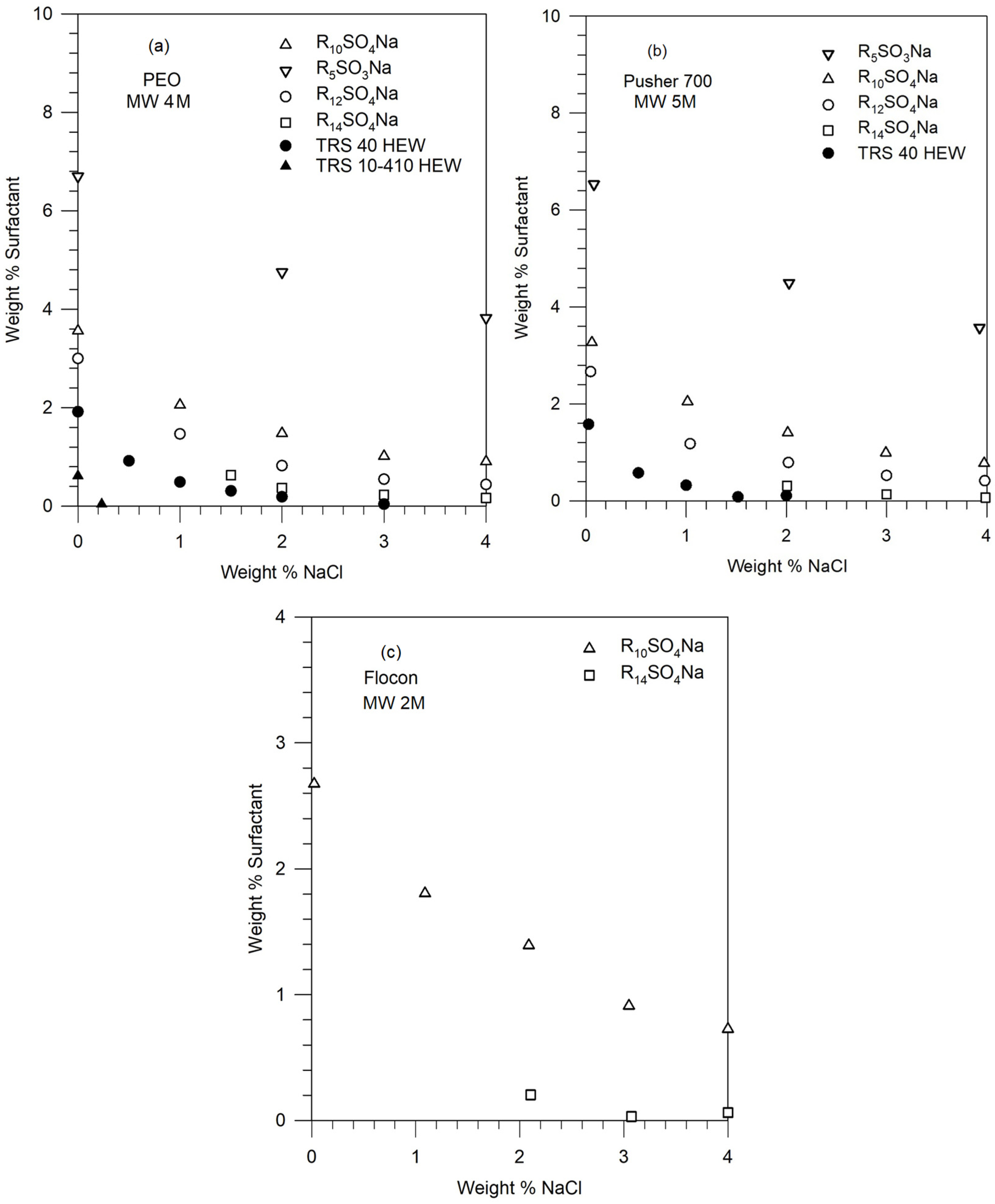
2. Experimental Study of Phase Behavior

2.1. Materials

The water-soluble polymers used in this study are listed in Table 1. The polyacrylamide and the biopolymer selected for the study here have been explored both in laboratory and field applications for enhanced oil recovery [2,7,8,9,10,11,12]. Pusher 700 is a partially hydrolyzed polyacrylamide with approximately 30% hydrolysis, and has an average molecular weight of 7 M. Flocon is an aqueous solution of the microbially produced heteropolysaccharide xanthan gum, with an average molecular weight of about 2 M. Polyethylene oxide (PEO) has been used in several studies of polymer–surfactant interactions and is a well-defined polymer for modeling studies, and a 4 M average molecular weight sample was used [10,12]. All are commercial samples which are expected to include a distribution of molecular weights.
Commercially available low molecular-weight anionic surfactants, as well as de-oiled petroleum sulfonates, were employed in this study. Table 2 lists the surfactants, their chemical structures, and the names of their suppliers.
The petroleum sulfonates supplied by Witco Chemical (TRS 40 and TRS 10-410) included a distribution of molecules as well as some amount of oil. These petroleum sulfonates were de-oiled and fractionated into two parts, one with a low average equivalent weight (LEW) and the other with a high average equivalent weight (HEW). The HEW samples were used for the phase behavior measurements [13]. Other surfactants were used as received from commercial suppliers and were reported to include a range of purity levels above 90%. For the petroleum sulfonates, the chemical formula is given, corresponding to a monosulfonate having the measured equivalent weight. The chemical structures of the polymer repeat units and the surfactants used in this study are presented in Figure 1.

2.2. Phase Behavior Measurements

Aqueous solutions of polymers with specified amounts of salt were prepared using either a magnetic stirrer or a propeller-type mixer. Care was taken to ensure that the maximum dispersion of polymer molecules was achieved without simultaneously causing any mechanical degradation. The viscosity of the polymer solution was measured prior to phase behavior studies to make sure that no polymer degradation had occurred. The solution of biopolymer (Flocon) was prefiltered through a Whatman No. 3 filter paper to remove any impurities and bacteria from the Flocon material before the phase behavior studies [13].
The desired amounts of surfactants were weighed in glass containers (bottles), to which a previously prepared polymer–electrolyte aqueous solution was added. The sample bottles were mixed with magnetic stirrers. The solutions were kept at room temperature (24 ± 2 °C) for phase behavior observations. The concentration boundaries which separate the one-phase region from the two-phase region for several polymer–surfactant systems were established based on two weeks of solution equilibration.
Figure 2 shows the phase boundaries for different surfactants in solutions of PEO (4 M), Pusher 700 (5 M), and Flocon (2 M). The points represent the experimentally observed compositions at which phase separation occurred. Note that the salt and surfactant concentrations are expressed as weight percent, that is, weight (in g) of the component in 100 g of the solution. These can be converted to molar concentrations, assuming that the total volume of the solution is practically that of water, given that the concentrations of the surfactant and the salt are not very large.
Figure 2 shows that for a given polymer molecule, the phase stability of the polymer–surfactant solution decreases (namely, phase separation occurs) with increasing equivalent weight of the surfactant, increasing salt concentration, and increasing surfactant concentration. For a given surfactant molecule, the phase stabilities for the polymers decrease in the order of PEO (4 M) ≥ Pusher 700 ≥ Flocon, but the differences among these high molecular-weight polymers are not very significant.

3. Development of a Pseudosolvent Model for Predicting Phase Behavior

3.1. The Pseudosolvent and Its Characteristic Energy ε 1 P *

An evaluation of polymer solution theories in the literature makes it apparent that an adequate predictive theory for a polymer–water system is presently not available [14,15,16,17]. The classical Flory–Huggins theory, given the original meaning of the Flory interaction parameter χ 12 [14], cannot predict the characteristic lower critical solution temperature (LCST) behavior exhibited by many aqueous polymer solutions, including the PEO–water system. When classical Flory theory is invoked, the interaction parameter is empirically fitted as a function of the temperature and the volume fraction of the polymer in solution to describe the experimentally observed phase behavior of the polymer–water systems [15,16,17]. This approach has no predictive capabilities.
The development of models for aqueous polymer solutions with true predictive capabilities is an area of continuing interest [18,19]. When the aqueous polymer solution also includes surfactant and electrolyte molecules, a formal molecular-level modeling of the four-component system becomes even more complex. Since the primary focus of this work is on predicting the phase behavior of these four component systems, a simplified approach tailored to treat phase behavior is proposed here.
In this approach, the pure solvent (water) is replaced by a pseudosolvent made up of water, electrolyte, and surfactant (present as both singly dispersed surfactant molecules and micellar aggregates). The polymer molecule is treated as the solute. In this manner, the four-component system is treated in terms of an equivalent pseudo two-component system.
Having defined the components, we need a polymer solution model as a framework to describe the pseudobinary system. For this purpose, we choose the lattice fluid model of polymer solutions developed by Sanchez and Lacombe [20,21,22,23,24]. This model is chosen because it allows representation of the LCST phase behavior and is thus capable of at least qualitatively or semi-quantitatively describing aqueous polymer solutions. It should be noted that the LCST behavior in the lattice fluid model emerges from the consideration of the presence of vacant sites in the lattice, and the resulting entropic effects. This is in contrast to the LCST behavior in aqueous polymer solutions that arises from hydrogen bonding interactions. Indeed, the lattice fluid model has been extended to account for hydrogen bonding [25], but for our purposes of just needing a polymer solution model framework, the basic lattice fluid model is adequate. The lattice fluid model for pure fluids and polymer solutions is briefly summarized in the Appendix A, together with all key equations used in this study.
In the lattice fluid model, a pure component is defined by three equation-of-state parameters: a characteristic energy ε * , a characteristic size of the component r, and a characteristic lattice site of hard-core volume v * . One can alternately use the characteristic pressure P*, characteristic temperature T*, and the characteristic density ρ * as the defining parameters (see Equations (A1)–(A4) in the Appendix A). For small molecules, the equation-of-state parameters for the pure components are usually estimated from experimental saturation vapor pressure data. The characteristic parameters for water determined in this way [20] are: P * = 26,520 atm, T * = 623 °K, and ρ * = 1.105 g/cm3; or equivalently, ε * = 1.238 kcal/mol, v * = 1.927 cm3/mol, and r = M/( ρ * v * ) = 8.45, the molecular weight of water M being 18. For high molecular-weight polymers, vapor pressures are negligibly small and therefore, the equation-of-state parameters are usually determined from experimental density data. Alternately, when only limited density data are available, the equation-of-state parameters can be determined from a single experimental density ρ, a thermal expansion coefficient α, and an isothermal compressibility β, at the same temperature and pressure, using Equations (A6) and (A7) in the Appendix A. For polyethylene oxide of molecular weight M, the equation-of-state parameters estimated by this single-point method [13] are P * = 3963 atm, T * = 597 °K, and ρ * = 1.202 g/cm3; or equivalently, ε * = 1.194 kcal/mol, v * = 12.36 cm3/mol, and r = M/( ρ * v * ). Note that the characteristic size parameter r is obviously dependent on the molecular weight M of the polymer.
For the pseudosolvent composed of water, the surfactant, and the electrolyte as the actual components, we assume that two of its equation-of-state parameters, v 1 * and r 1 , (subscript 1 denotes the solvent and subscript 2 denotes the polymer) are identical to those of water. The third parameter, characteristic energy ε 1 P * (the subscript 1P is introduced to distinguish it from 1, used for water) is taken to be different from that of water and is assumed to account for all the surfactant–electrolyte composition-dependent characteristics of the pseudosolvent. Thus, the critical postulate underlying our pseudosolvent model is the assumption that a single characteristic energy parameter ε 1 P * contains all the information related to the type and amounts of surfactant and electrolyte molecules present in water. It should be mentioned that this is an ad hoc extra-thermodynamic postulate, and is justified only a posteriori by the resulting simplicity of the thermodynamic approach and the usefulness of the results.

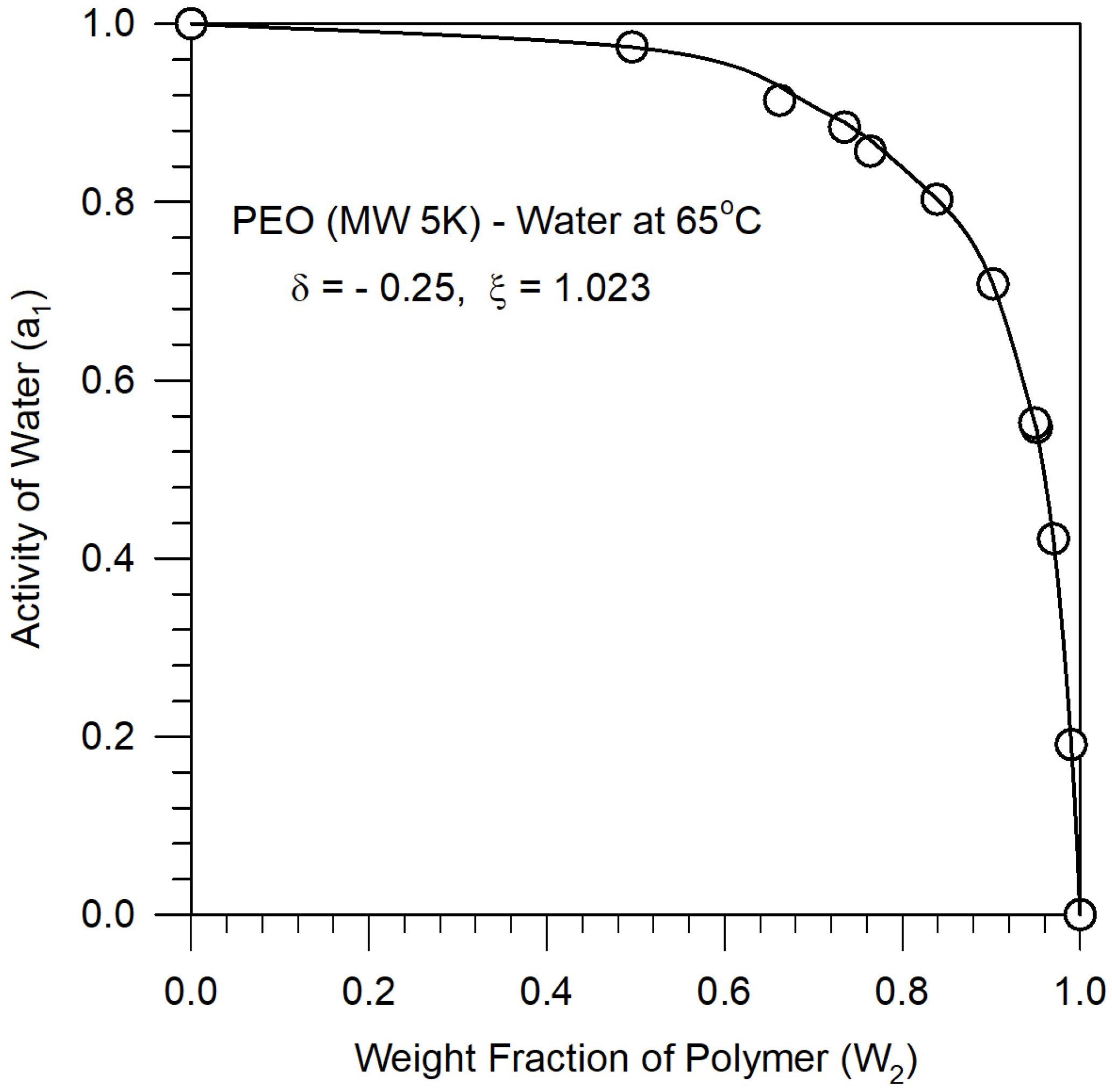
3.2. Polymer–Pseudosolvent Binary Parameters ξ and δ

For the binary polymer–pseudosolvent solution, two additional parameters characteristic of the mixture properties are introduced, as is common in many theories of solutions, to account for non-idealities of mixture behavior. The binary energy parameter ξ represents the deviation of the interaction energy from the geometric mean rule and the binary volume parameter δ represents the deviation of the close-packed mixture volume from the arithmetic additivity rule. The introduction of binary parameters ξ and δ adds considerable flexibility to the lattice fluid model for mixtures, as it does in all solution models in the literature. The binary parameters for the polymer–pseudosolvent are assumed to be the same as for polymer–water and are determined from experimental thermodynamic data on polymer–water solutions. The estimates for the binary parameters obtained from different solution properties, such as activity of the solvent, heat of mixing, or volume change on mixing are generally not identical, reflecting the fundamental inadequacies in the current state of the theory of the liquid state. Since we are interested in the polymer solution phase behavior, we use the water activity data to estimate the binary polymer–water parameters. As shown in Figure 3, the experimental activity data [26] for a PEO–water system is fitted well by the theoretical water activity calculated from Equation (A13) in the Appendix A, for the binary parameter values ξ = 1.023 and δ = −0.25. These binary parameters are taken to be independent of temperature.

3.3. Polymer–Pseudosolvent Phase Diagram in the Parametric Space of
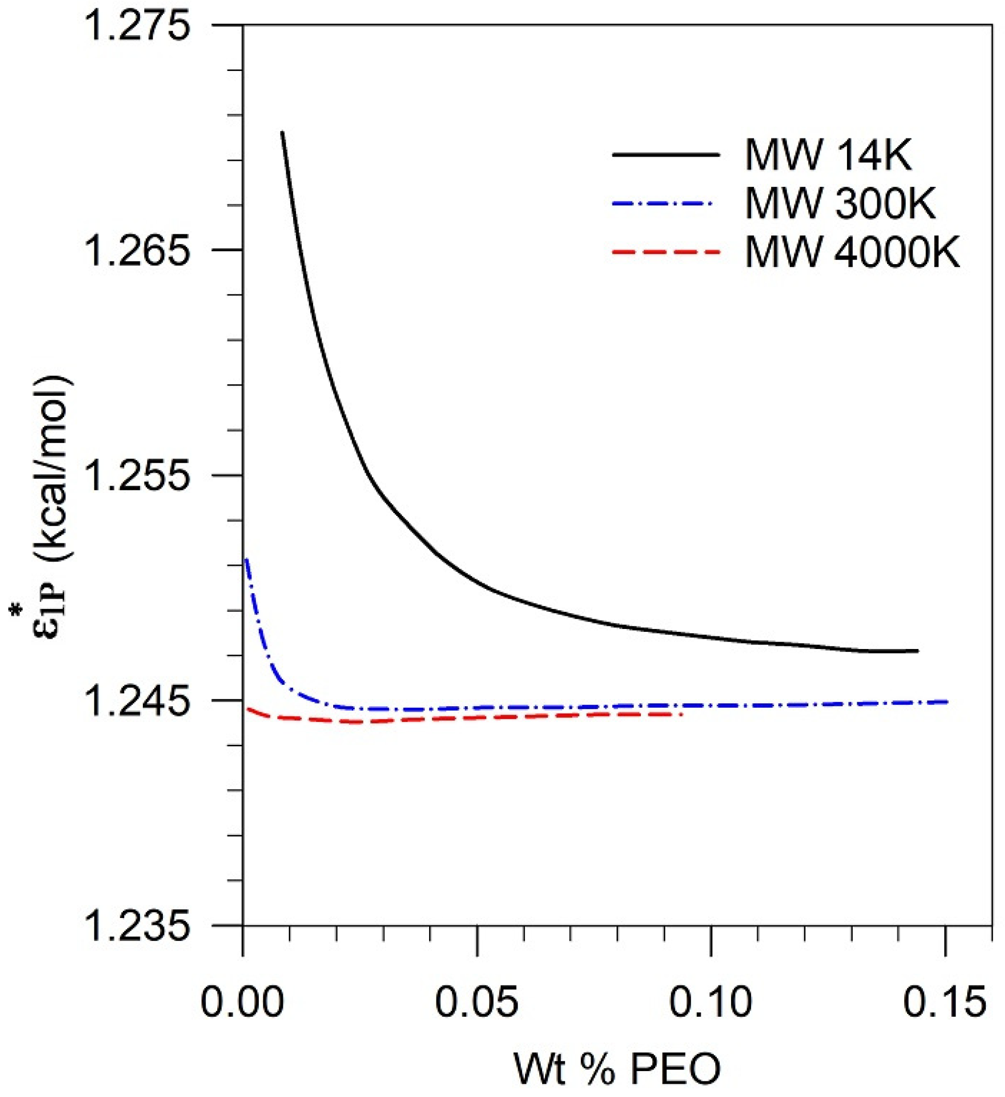
 ε 1 P *

Given the equation-of-state parameters ε 2 * , v 2 * , and r 2 for the polymer, the two equation-of-state parameters, v 1 * and r 1 , associated with the pseudosolvent (assumed to be the same as for water), and the binary parameters ξ and δ for the polymer–pseudosolvent (assumed to be the same as for polymer–water), one can calculate the phase behavior of the polymer solution for various pseudosolvents characterized by differing values for ε 1 P * . The phase stability criteria are summarized in Equations (A20)–(A23) in the Appendix A. Since the equation-of-state parameters, as well as the binary polymer–water interaction parameters, are known for polyethylene oxide, we were able to construct the polymer–pseudosolvent phase diagram shown in Figure 4 for three different molecular weights of PEO (14 K, 300 K and 4 M) in the ε 1 P * vs. polymer concentration space. The phase diagram shows that while the characteristic parameter ε 1 P * of the pseudosolvent is below a certain value, the polymer–pseudosolvent solution is stable; and when ε 1 P * is above a certain value, the solution is unstable. The characteristic energy of the pseudosolvent ε 1 P * at which phase separation occurs is a function of the polymer molecular weight and the concentration of the polymer in solution, as well as the temperature. Similar phase diagrams can be constructed for other polymers of interest, when their equation-of-state parameters and their binary interaction parameters with water are known.
Figure 4 shows that for high molecular-weight polymers, PEO (4 M) and PEO (300 K), the value of ε 1 P * at the phase boundary is almost constant in the polymer concentration range of 100 ppm to 1500 ppm (equivalently, 0.01 wt% to 0.15 wt%). In contrast, for the low molecular-weight polymer PEO (14 K), the value of ε 1 P * is significantly higher than that for the high molecular-weight polymer, especially at low polymer concentrations.

3.4. Mapping the Characteristic Energy ε 1 P * of the Pseudosolvent to Its Composition

The characteristic energy ε 1 P * of the pseudosolvent needs to be translated to the actual composition of the pseudosolvent (namely, the chemical structures and concentrations of the surfactant and the electrolyte). This is accomplished by considering the free energy difference ΔG between the pseudosolvent and water. In the formalism of the lattice fluid model, given the equation-of-state parameters for a pure fluid, the free energy G of a pure fluid can be calculated using Equation (A1) in the Appendix A by introducing within it the fluid density calculated from the equation of state, Equation (A4). Consequently, the free energy difference ΔG between the pseudosolvent and water is calculated as follows:
Δ G = G ( ε 1 P * , v 1 * , r 1 ) G ( ε 1 * , v 1 * , r 1 )
The calculated relation between ΔG and ε 1 P * is presented in Figure 5. Note that this relation is independent of the polymer and is thus a universal relation for pseudosolvents in the framework of the lattice fluid model and can be used to explore the phase behavior involving any polymer.
The characteristic energy parameter for water ε 1 * is 1.238, at which ΔG = 0. For ε 1 P * < ε 1 * , ΔG > 0, and for ε 1 P * > ε 1 * , ΔG < 0. The characteristic energy parameter is a measure of the cohesive energy of the solvent. The higher the energy parameter, the larger the cohesive energy of the solvent and the greater the probability of polymer exclusion, and therefore the likelihood of phase separation is larger.

4. Calculation of ΔG from Thermodynamic Data on Surfactants and Electrolytes

The thermodynamic quantity of interest for predicting the phase behavior of a polymer–surfactant–electrolyte-water system, in the framework of the pseudosolvent concept, is the free energy difference ΔG between the pseudosolvent and pure water. We need to develop a quantitative relation between ΔG (which is taken to represent, through its magnitude, all the essential characteristics of the pseudosolvent) and the actual chemical composition of the pseudosolvent. The free energy difference ΔG can be related to the actual chemical composition of the pseudosolvent using thermodynamic models and data (entirely independent of the polymers) available in the literature for surfactant and electrolyte solutions, as detailed in this section. The ΔG can be calculated for different surfactants and electrolytes, as
Δ G = G ( water + surfactant + electrolyte ) G ( water )
In this manner, the actual composition of the pseudosolvent can be related to the free energy difference ΔG and thereby to the characteristic energy parameter ε 1 P * of the pseudosolvent.
As mentioned earlier, the pseudosolvent consists of surfactant molecules, any electrolyte added, and water. The surfactant molecules are present both in their singly dispersed state and in the form of micellar aggregates. The pseudosolvent can be thought of as a mixture of water (component 1) in its pure water reference state with the other components, electrolyte counterion (component 2), electrolyte co-ion (component 3), surfactant counterion (component 4), and surfactant co-ion (component 5) in their infinitely dilute reference states. Since components 2 and 3 come from the salt and components 4 and 5 come from the surfactant, their mole fractions x or molar concentrations C are related as x2 = x3 and x4 = x5, or, equivalently, C2 = C3 and C4 = C5. Expressions for estimating the magnitude of ΔG are developed in this section.

4.1. Water + Electrolyte Systems

For the aqueous electrolyte solutions, we adopt the treatment of Kawaguchi et al. [27], formulated based on the Analytic Solution of Group (ASOG) model [28], to calculate the activity of the components. In this treatment, the electrolyte solution is considered to consist of free water molecules (W), hydrated cations (C), and hydrated anions (A). The electrolyte is assumed to be dissociated completely to produce the cations and the anions with which water molecules are bound. The structure of the hydrated ion is determined by the number of hydration water molecules around it. A hydration water molecule is distinguished from a free water molecule because the water of hydration is tightly bound, such that its motion and intramolecular states are different from those of the free water. The hydrated cation (nC water molecules and a cation) and the hydrated anion (nA water molecules and an anion) are treated as the two solute components present in the solvent water. Using this visualization, the activities of the components of the electrolyte solution can be viewed as being composed of (i) the ideal entropy of mixing; (ii) an excess entropic contribution arising from the presence of the hydrated anions, the hydrated cations, and the free water molecules, described using the Flory–Huggins expression [14]; (iii) an enthalpic contribution arising from the interactions between the free water and the hydration water molecules that surround the ions; and (iv) long-range ion–ion electrostatic interactions. Therefore, the activity of component i can be written as
a i = x i γ i = x i γ i FH γ i G γ i EL
where x i is the mole fraction of component i (i refers to the free water, hydrated cation, and hydrated anion), γ i is the activity coefficient, and γ i FH , γ i G , and γ i EL are the excess entropic, enthalpic, and electrostatic contributions due to the non-idealities.
The expression for the excess entopic contribution to the activity coefficient is given by the ASOG model [27], as follows:
ln γ i FH = ln ( ν i / j x j h ν j ) + 1 ( ν i / j x j h ν j )
In Equation (4), x i h is the mole fraction of component i in the mixture, with the superscript h denoting that the water of hydration is treated as an integral part of the species. ν i is the number of atoms (other than hydrogen) in the component i and equals 1, ( n C + 1), and ( n A + 1), for free water, hydrated cation, and hydrated anion, respectively. Accounting for the hydrated water surrounding the ions, the mole fractions of free water ( x W h ), hydrated electrolyte cation ( x C h ), and hydrated electrolyte anion ( x A h ) are given by
x W h = x W n C x C n A x A x W n C x C n A x A + x C + x A , x C h = x C x W n C x C n A x A + x C + x A , x A h = x A x W n C x C n A x A + x C + x A
where x W , x C , and x A are the actual mole fractions of the water, the electrolyte cation, and the electrolyte anion in solution. If we consider only a water–electrolyte solution, in the notations introduced for all components of the pseudosolvent, x W = x 1 , x C = x 2 , and x A = x 3 . Equation (5) refers to a single cation and a single anion, but if there are multiple distinct ions, they can be accounted for through additional terms for each distinct ion.
The enthalpic contribution to the activity coefficient in the ASOG model [27] is expressed as
ln γ i G = k ν ki ( ln Γ k ln Γ k ( i ) ) ln Γ k = ln ( e q e h a k / e ) + 1 e ( q e h a e / k / m q m h a e / m ) q k = k x i h ν ki / i x i h k ν ki
where ν ki is the number of interacting groups of kind k in component i, Γ k is the activity coefficient of the interacting group k in the mixture, Γ k ( i ) is the standard state activity coefficient of group k, and q k is the group fraction of group k. The expression for the activity coefficient for group k, Γ k , follows the Wilson model [29].
There are only two interacting groups in this system, namely, the free water (denoted by subscript k = OH) and hydrated water (k = OH*), since the interaction between water molecules and ions is entirely accounted for solely through this hydration. Each component has only one kind of group in it: k = OH in free water, and k = OH* in hydrated cation and in hydrated anion. The group activity coefficients are given [27] by
ln Γ OH = ln ( q OH + q OH * a OH / OH * ) + 1 ( q OH q OH + q OH * a OH / OH * + q OH * a OH * / OH q OH a OH * / OH + q OH * ) ln Γ OH * = ln ( q OH * + q OH a OH * / OH ) + 1 ( q OH * q OH * + q OH a OH * / OH + q OH a OH / OH * q OH * a OH / OH * + q OH )
In Equation (7), a OH / OH * and a OH * / OH are the Wilson interaction energy parameters and q k is the group mole fraction of group k. For water, the standard state is pure water and for the anion and the cation, the standard state is the infinite dilution condition. Therefore, from Equation (7),
Γ OH ( i ) = 0 , ln Γ OH * ( i ) = ln a OH / OH * + 1 a OH * / OH
Kawaguchi [27] has reported the hydration numbers of 11 ions and the interaction energy parameters ( a OH / OH * and a OH * / OH ) between the free water denoted by OH and the hydration water denoted by OH*. These parameter estimates were obtained by correlating the activities of water in electrolyte solutions very accurately, taking ν ki in Equation (6) as 1.6 for free water, n C for the hydrated cation, and n A for the hydrated anion [27,30]. For 14 electrolyte solutions with 1:1 and 2:1 electrolytes, the activities of water calculated by the ASOG model using these optimized parameters were found, on average, to deviate by less than 1% from the experimental data [31] for salt concentrations of up to 5 molality [27]. Therefore, we directly make use of the parameter estimates reported in Kawaguchi’s work.
The interaction energy parameters a OH / OH * and a OH * / OH , where OH denotes a free water and OH* a hydration water, were determined to be 1.82 and 1.78, respectively [27,30]. Note that the interaction parameters between identical groups will be a unity, namely, a OH / OH = a OH * / OH * = 1. The values of the hydration numbers n C and n A , optimized by Kawaguchi by fitting the water activity data, are presented in Table 3. The value of n C decreases with the increase of ionic radius. This tendency qualitatively coincides with that anticipated based on reference [31] in the literature.
As mentioned earlier, in the ASOG model for electrolyte solutions, the short-range interactions between water molecules and ions are accounted for entirely through the model of hydration. The long-range electrostatic contribution to the activity coefficient γ i EL is calculated using an expression derived from the Fowler–Guggenheim theory [32]:
ln γ i EL = v i ¯ 24 π N A r o 3 ( κ r o ) 3 σ ( κ r o ) σ ( κ r o ) = 3 ( κ r o ) 3 1 + κ r o 1 1 + κ r o 2 ln ( 1 + κ r o ) κ = 4 π e 2 N i Z i 2 ε kT 1 / 2
In Equation (9), v i ¯ is the partial molar volume of component i, NA is the Avogadro number (6.022 × 10²³), ro is the ion size parameter, κ is the inverse Debye length, ε is the dielectric constant of water (78 at 298 °K), Ni is the number/cm3 concentration of the ion i, and Zi is the number of charges on the ion i. Taking v i ¯ = 18 cm3/mol and ro = 4 × 10⁻⁸ cm, Kawaguchi calculated the activity of water in NaCl solutions and found that this contribution is negligibly small compared to the other contributions (see Figure 3 of Ref. [27]). Our calculations confirm that γ i EL for water changes from 1.000 at 0 M NaCl to 1.0037 at 1 M NaCl and 1.0074 at 2 M NaCl, indicating only a very small contribution from this term.
In the Kawaguchi treatment of electrolyte solutions, the hydrated anion and cation are taken as the distinct chemical species used to develop expressions for the activity coefficients. But in the pseudosolvent model, we treat the electrolyte ions in the unhydrated state as the components. Therefore, while writing an expression for the free energy difference ΔG between the pseudosolvent composed of water + electrolyte and water, we should introduce a correction term ΔGref to account for this difference in the reference states. On this basis, the free energy difference ΔG between the pseudosolvent composed of water + electrolyte and pure water can be written as
Δ G = RT [ x 1 ln x 1 + x 2 ln x 2 + x 3 ln x 3 ] + RT [ x 1 ln ( γ 1 FH γ 1 G γ 1 EL ) + x 2 ln ( γ 2 FH γ 2 G γ 2 EL ) + x 3 ln ( γ 3 FH γ 3 G γ 3 EL ) ] + x 2 Δ G ref
The correction term ΔGref accounts for the change in energy when unhydrated ions become hydrated with associated water molecules. This process involves the breaking of water–water hydrogen bonds and replacement by ion–dipole interactions between the ion and water. The corresponding energy changes cannot be unambiguously estimated, and we have assumed a value of 5000 cal/mole based on typical magnitudes for hydrogen bonding energies (which can range between 2 to 10 kcal/mole) and ion–dipole interactions reported in the literature. We present computed results which show the sensitivity of the calculated free energy difference ΔG between the pseudosolvent and water to variations in this assumed value. All other parameters for calculating ΔG in Equation (10) have been established and validated by Kawaguchi [27] based on accurate fitting of water activity data for numerous electrolyte solutions over a wide range of concentrations.

4.2. Water + Surfactant Systems

The surfactant solution is composed of water (component 1), surfactant counterion (component 4), and surfactant co-ion (component 5). The formation of micelles in the solution can be formally represented by the law of mass action as
m S + n A + ( SA ) ( m n )
where S represents the free surfactant ion (representing an anionic surfactant, and this can be similarly written for cationic surfactants), A+ represents the free counterion, m is the aggregation number of the micelle, and n is the number of counterions bound to the micelle surface. Below the critical micelle concentration (CMC), the surfactant molecules are mostly present in the singly dispersed form, and above the CMC, the added surfactant molecules appear as micellar aggregates (denoted by the subscript mic). The singly dispersed surfactant is completely dissociated into surfactant counterion (denoted as 4S) and surfactant co-ion (denoted as 5S). The activity of the surfactant in solution is equal to the activity of the singly dispersed surfactant because of the monomer–micelle equilibrium.
The free energy difference ΔG between the surfactant solution (pseudosolvent) and pure water can be written, similar to Equation (10), in the form
Δ G = RT [ x 1 ln ( x 1 ) + x 4 ln ( x 4 S ) + x 5 ln ( x 5 S ) + x mic ln ( x mic ) ] + RT [ x 1 ln ( γ 1 S ) + x 4 ln ( γ 4 S S ) + x 5 ln ( γ 5 S S ) + x mic ln ( γ mic S ) ]
where the superscript S is added to indicated that these activity coefficients appear in surfactant solutions. In Equation (12), x mic and γ mic S refer to the mole fraction and activity coefficient for micelles. The monomer–micelle equilibrium, Equation (11), implies that the micelle activity can be related to the monomer activity in the form
ln ( x mic γ mic S ) = m ln ( x 5 S γ 5 S S ) + n ln ( x 4 S γ 4 S S )
Further, the concentration of singly dispersed surfactant and micelles can be related to the total concentration via the mass balance
x 4 = x 4 S + n x mic , x 5 = x 5 S + m x mic
Introducing Equations (13) and (14) into Equation (12), we have
Δ G = RT [ x 1 ln ( x 1 ) + x 4 ln ( x 4 S ) + x 5 ln ( x 5 S ) ] + RT [ x 1 ln ( γ 1 S ) + x 4 ln ( γ 4 S S ) + x 5 ln ( γ 5 S S ) ]
The amount of the free surfactant ions x 5 S can be estimated from the critical micelle concentration, CMC. The mole fraction of surfactant in the solution near the CMC is generally quite small, and hence the total number of moles in 1 L of solution can be approximated as 55.5 moles, based on water alone. Therefore, with the CMC expressed as a molar concentration (mole/L), we can estimate
x 5 S = CMC / 55.5
The CMC of homologous straight-chain ionic surfactants in aqueous medium, in the absence of any added salt (C2 = 0), displays a dependence on the number of carbon atoms N in the hydrophobic chain in the form
ln CMC C 2 = 0 = A B N
where A and B are constants [33].
The number of counterions binding on the micelles depends on the concentration of counterions in the solution. The binding of counterions on the micelles is assumed to follow the simple Langmuir adsorption isotherm. Correspondingly, the degree of dissociation of the micelle, denoted by α, can be written as
α = m n m = α * 1 + K ad I , I = C i Z i 2 2 = ( C 4 S + C 5 S + ( δ α m ) 2 ( C 5 C 5 S ) / m ) 2 I = 55.5 ( x 4 S + x 5 S + ( δ α m ) 2 ( x 5 x 5 S ) / m ) 2
In Equation (18), α* is the degree of dissociation of micelles in an infinitely dilute solution, K ad is the Langmuir adsorption equilibrium constant (L/mole) for counterion binding to micelles, I is the ionic strength of the solution, x 4 S , x 5 S are the mole fractions and C 4 S , C 5 S are the molar concentrations of the counterion and co-ion of the free surfactant, respectively, and ( C 5 C 5 S ) / m is the molar concentration of micelles of aggregation number m. Below the CMC, x 4 S = x 4 , x 5 S = x 5 . Above the CMC, x 5 S = CMC/55.5 and x 4 S = x 5 S + α ( x 5 x 5 S ) .
In the absence of any added electrolyte, the ionic strength is determined by the concentration of the singly dispersed surfactant, which is dissociated into surfactant co-ion and surfactant counterion (the first two terms in the expression for I), and the micelles which contain (αm) multiple charges (the last term in the expression for I). It is generally assumed that the charges on the micelles are partially shielded, and the shielding factor δ < 1 is introduced to reduce the effect of the micellar charge on the ionic strength of the solution. It has been found that using δ = 1 is not in agreement with the experimentally determined values of activity and osmotic coefficients. For several ionic surfactants, δ is estimated to be around 0.5 [34], and that value is assumed in this work.
The activity coefficient of the surfactant co-ion and the surfactant counterion are difficult to determine independently, and the experimental measurements usually focus on an average activity coefficient, defined as γ ± S S = ( γ 4 S S γ 5 S S ) 1 / 2 [34,35]. There is very little data in the literature on experimentally determined average activity coefficients for surfactants. The average activity coefficient of the surfactant in the presence of ionic species is attributed mainly to the “salting out” or “salting in” of the hydrophobic group of the surfactant in the aqueous solvent. For nonpolar solutes in aqueous electrolyte solutions of ionic strength I, McDevit and Long [36] developed a theoretical expression for the activity coefficient in the form ln γ = k S I . This linear dependence is identical to the well-known empirical Setschenow relation [37], with k S designated as the Setschenow constant. Although the equation of McDevit and Long was developed for nonpolar solutes, it has been applied to various polar and polar organic compounds [38], and nonionic surfactants [39] as well. To retain simplicity, we will assume that this relation can be applied to calculate the average activity coefficient of the surfactant.
ln γ ± S S = k S I
The activity coefficient of water γ 1 S can then be derived through the Gibbs–Duhem equation. When the molar concentration of the surfactant C 5 is less than the CMC, no micellization occurs. When C 5 is greater than the CMC, γ 1 S includes contributions arising from the presence of micelles. One thus determines the surfactant contribution to the activity coefficient of water to be
ln γ 1 S = k S C 5 2 C 1   when   C 5 < CMC ln γ 1 S = k S CMC 2 C 1 k S α 2 C 1 ( C 5 2 CMC 2 ) + 1 C 1 ( C 5 CMC ) + ( 1 α ) CMC C 1 α ln ( C 5 α + ( 1 α ) CMC CMC )   when   C 5 > CMC
The free energy difference ΔG between the water + surfactant solution (pseudosolvent) and pure water can now be calculated from Equation (15) by introducing Equations (16) to (20) within it.

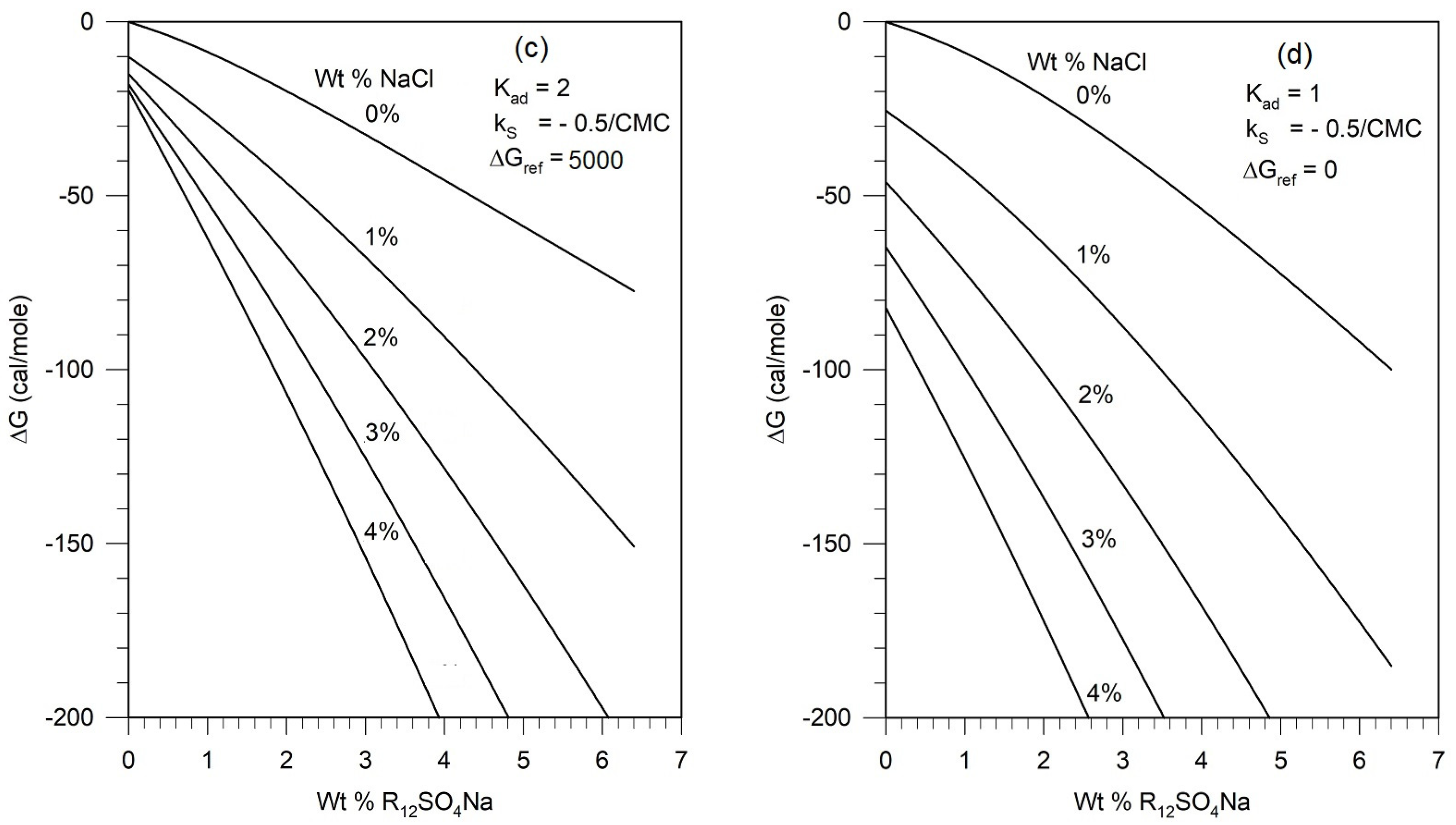
4.3. Water + Surfactant + Electrolyte Systems

For water–surfactant–electrolyte solutions, the expression for the free energy difference ΔG between the pseudosolvent and pure water can be written by extending Equation (10) for the free energy difference of the water + electrolyte system and Equation (15) for the free energy difference of the water + surfactant system. On this basis, we can write
Δ G = RT [ x 1 ln x 1 + x 2 ln x 2 + x 3 ln x 3 + x 4 ln x 4 S + x 5 ln x 5 S ] + RT [ x 1 ln ( γ 1 FH γ 1 G γ 1 EL γ 1 S ) + x 2 ln ( γ 2 FH γ 2 G γ 2 EL ) + x 3 ln ( γ 3 FH γ 3 G γ 3 EL ) + ( x 4 + x 5 ) ln γ ± S S ] + x 2 Δ G ref
As mentioned earlier, subscripts 2 and 3 refer to the counterion and the co-ion of the electrolyte. Subscripts 4 and 5 refer to the counterion and the co-ion of the surfactant. The γ i FH contribution is calculated from Equation (4), the γ i G contribution from Equation (6), the γ i EL contribution from Equation (9), the γ ± S S contribution from Equation (19), and the γ 1 S contribution from Equation (20). When the counterion of the electrolyte and the counterion of the surfactant are not different but identical, the entropy of mixing term is modified, and we have
Δ G = RT [ x 1 ln x 1 + ( x 2 + x 4 ) ln ( x 2 + x 4 S ) + x 3 ln x 3 + x 5 ln x 5 S ] + RT [ x 1 ln ( γ 1 FH γ 1 G γ 1 EL γ 1 S ) + x 2 ln ( γ 2 FH γ 2 G γ 2 EL ) + x 3 ln ( γ 3 FH γ 3 G γ 3 EL ) + ( x 4 + x 5 ) ln γ ± S S ] + x 2 Δ G ref
The ionic strength I includes contributions from the surfactant and the added electrolyte.
I = ( C 2 + C 3 + C 4 S + C 5 S + ( δ α m ) 2 ( C 5 C 5 S ) / m ) 2 I = 55.5 ( x 2 + x 3 + x 4 S + x 5 S + ( δ α m ) 2 ( x 5 x 5 S ) / m ) 2
The CMC of the surfactant decreases in the presence of the electrolyte in the aqueous solution, and this will influence the concentrations x 4 S and x 5 S . The depression of CMC in ionic surfactant solutions is due mainly to the decrease in the thickness of the ionic double-layer surrounding the ionic head groups in the presence of the additional electrolyte and the consequent decrease in the electrostatic repulsions between them at the micelle surface. Experimental data [40] suggest that for ionic surfactants, the effect of the concentration of electrolyte on the CMC is given by
ln CMC C 2 ln CMC C 2 = 0 = a [ ln ( C 2 + CMC C 2 = 0 ) ln ( CMC C 2 = 0 ) ]
where a is a constant for a given ionic head group at a particular temperature and is independent of the hydrophobic tail length, and C 2 is the concentration of the added electrolyte in moles per liter. Introducing Equation (17) into Equation (24), we can calculate the CMC for a surfactant with N carbon atoms in the hydrophobic tail at an added electrolyte concentration of C 2 from
ln CMC C 2 = ( 1 + a ) ( A BN ) a ln ( C 2 + A BN )

4.4. Estimation of Thermodynamic Parameters from Literature

For calculating the free energy difference ΔG between the pseudosolvent (composed of water–surfactant–electrolyte) and the pure water using Equation (22), the values of the following thermodynamic parameters for the surfactant–electrolyte solutions are needed.
(a)
A and B in Equation (17) for the hydrophobic tail length-dependence of the CMC;
(b)
a in Equation (24) for the ionic strength-dependence of the CMC;
(c)
K ad and α* in Equation (18) for counterion binding at the micellar surface;
(d)
k S in Equation (19) for the activity coefficient of the surfactant.
The parameters A and B in Equation (17), used for calculating the critical micelle concentration as a function of surfactant chain length, in the absence of any added salt, are 3.45 and 0.69 for alkyl sulfates, and 3.68 and 0.67 for alkyl sulfonates and alkylbenzene sulfonates [40]. Parameter a in Equation (24), used to calculate the effect of salt on the CMC for sodium alkyl sulfate and sulfonates, is 0.458 [40,41]. All of these parameter values are based on expressing the CMC in units of molar concentration (moles/L). The CMC values of surfactants with different hydrocarbon chain lengths and at various added salt concentrations can be readily calculated from Equation (25), incorporating the values for A, B, b, N, and C 2 .
The micelle aggregation number m appearing in Equations (18) and (23) is taken to be 50 for all surfactants considered here, to avoid adding additional parameters. Changing the value of m does not significantly affect the computed free energy differences or the phase diagrams. The adsorption constant K ad in Equation (18) for the counter-ion adsorption at the micellar surface is taken as 1.0 (mole/L)−1, and α* in Equation (18) is taken to be 0.5. Both the value of K ad and the value of α* are chosen to agree with the experimental observation that the fraction of the counter-ions’ dissociation on the micelle surface, for alkyl sulfonates and alkyl sulfates, is in the range of 0.3 to 0.6 for the surfactant and electrolyte concentrations studied [33,41,42].
For alkyl sulfonate and alkyl sulfate surfactants, experimental average activity coefficient data are not available for the homologous series of surfactants. Experimental data for short chain alkyl carboxylates [35] suggest that the mean molar activity coefficients for different carboxylate homologs approach a constant value of −0.25 at their critical micellar concentrations. If this behavior is displayed by the alkyl sulfates and sulfonates, the Setschenow constant k S for differing hydrophobic chain lengths can be estimated from the following equation:
ln γ ± S S ( at CMC ) = ks   CMC = constant
For the present study, the value of this constant in Equation (26) for alkyl sulfate, alkyl sulfonate, and alkyl benzene sulfonate surfactants is chosen to be −0.5, since it is in the range of the experimental average activity coefficient for sodium dodecyl sulfate [34,42,43]. Incorporating this constant value of −0.5 and the cmc calculated as described above, the Setschenow constant kS is determined using Equation (26). The validity of Equation (26) for other surfactants (in other words, whether γ ± S S at CMC is equal to a constant value for surfactant homologs) needs experimental verification. However, at the present time, due to a lack of experimental activity coefficient data for various surfactant homologs, the validity of Equation (26) is assumed, and a constant value of −0.5 is assigned to calculate the values of k S for alkyl sulfate, alkyl sulfonate, and alkyl benzene sulfonate surfactant homologs.
Since the parameters K ad , α*, and k S have been assigned values which are reasonable, but without any direct supporting experimental data for the specific molecular systems, we perform parametric sensitivity analysis in Section 5.4 on how changes in these parameter values affect the calculation of the free energy difference ΔG, and thereby the phase diagram.

5. Phase Behavior Predictions and Construction of Phase Diagrams

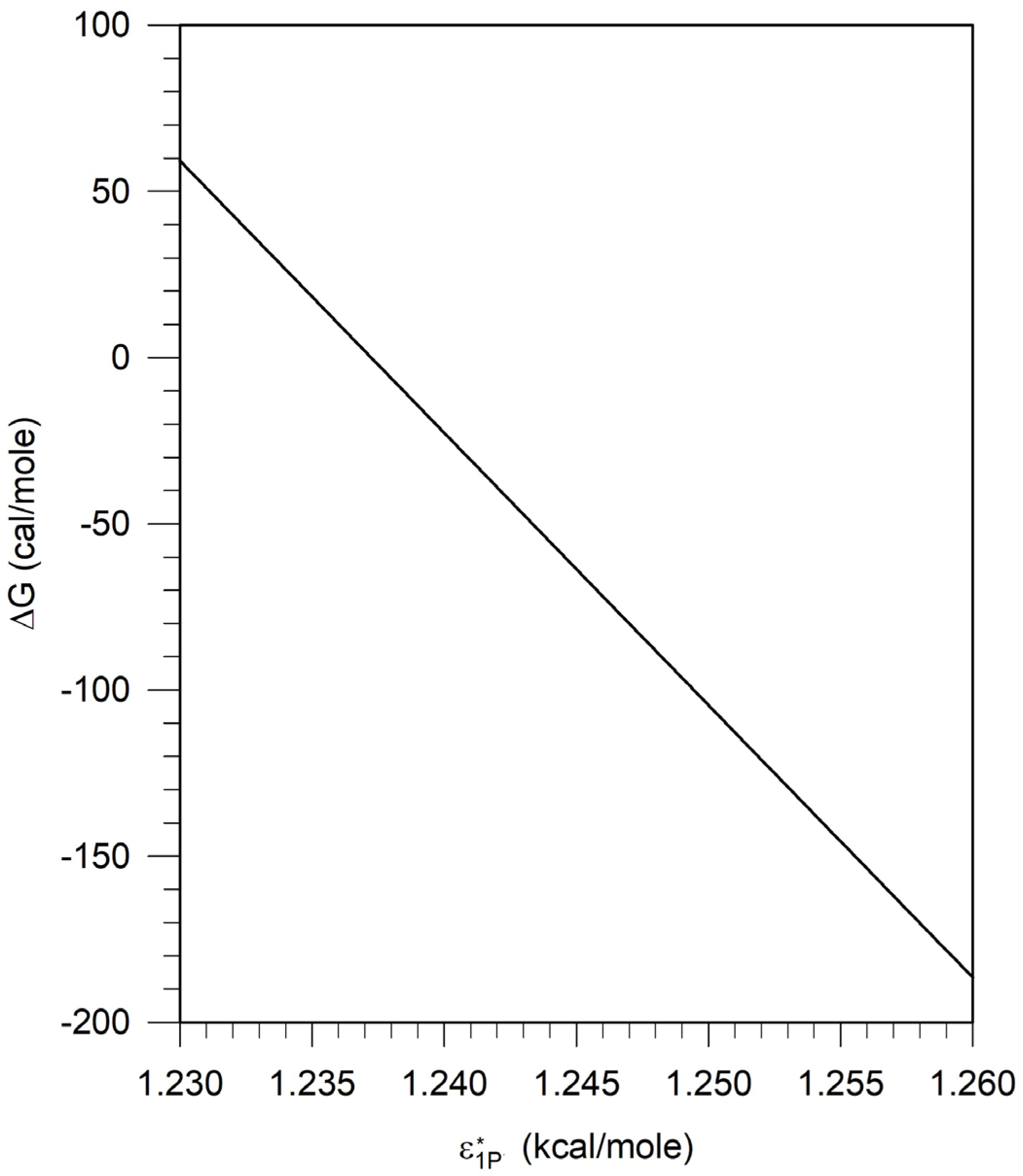
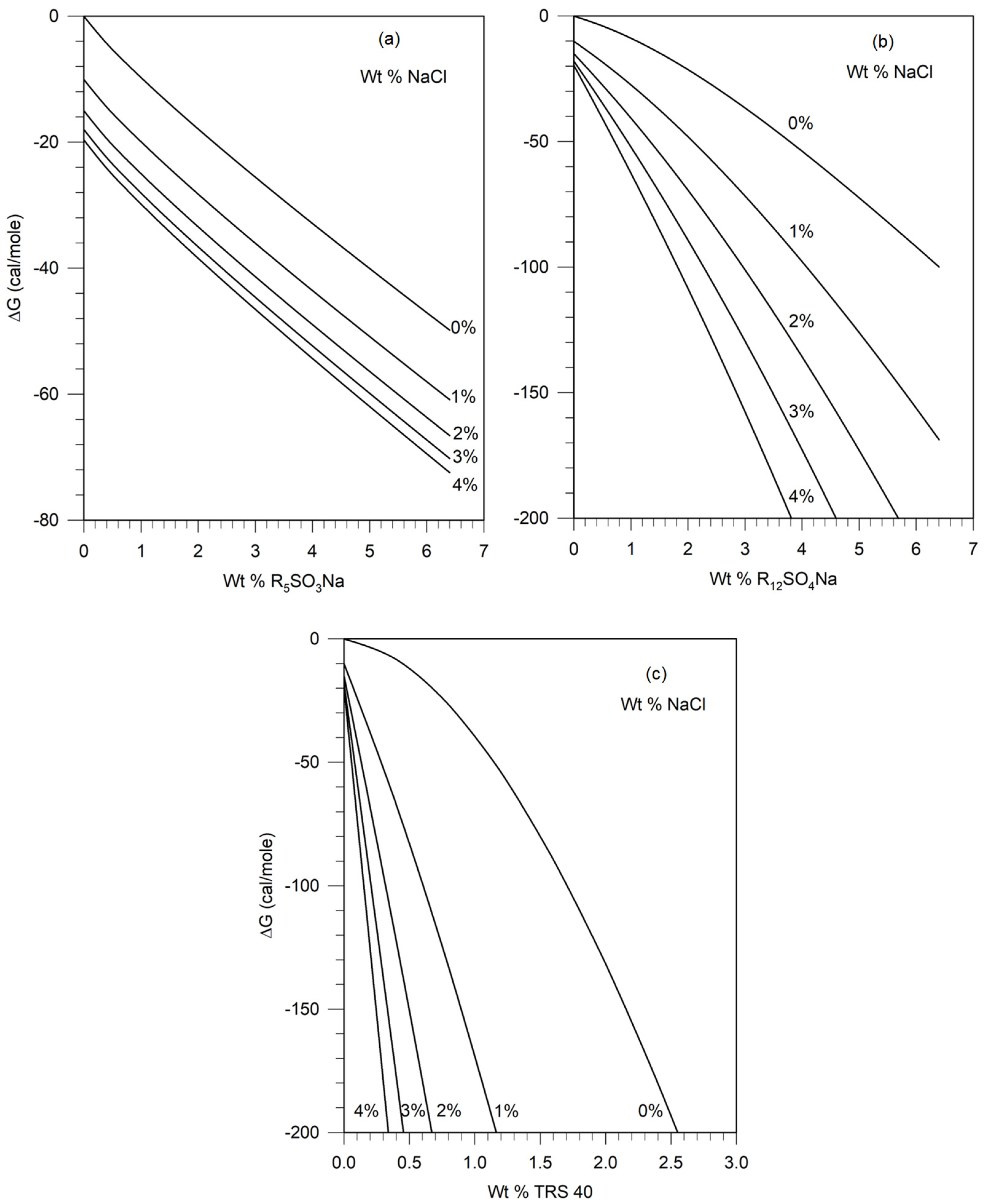
5.1. Calculation of the Free Energy Difference between the Pseudosolvent and Water

The free energy difference ΔG defined in Equation (22) has been calculated for sodium pentyl sulfonate (R5SO3Na), sodium decyl sulfate (R10SO4Na), sodium dodecyl sulfate (R12SO4Na), sodium tetradecyl sulfate (R14SO4Na), TRS 40 HEW (RB17SO3Na), TRS 10-410 HEW (RB24SO3Na), and TRS 18 HEW (RB34SO3Na) at different salt and surfactant concentrations using the parameter values provided above. For illustrative purposes, we have plotted, in Figure 6, the calculated values of ΔG for the pseudosolvent containing sodium pentyl sulfonate, sodium dodecyl sulfate and TRS 40 as surfactants and sodium chloride as the electrolyte, in the concentration range of interest. Similar plots have been constructed for each of the surfactants mentioned above, using NaCl as the electrolyte in all cases.
Figure 5, discussed earlier, in Section 3.3, shows the relation between the characteristic energy parameter ε 1 P * of the pseudosolvent and the free energy difference ΔG between the pseudosolvent and water, calculated from Equation (A1), in the framework of the lattice fluid theory. Figure 5 shows that as ε 1 P * increases, ΔG decreases. The implication of this for the calculated results shown on Figure 6 is that the characteristic energy parameter ε 1 P * of the pseudosolvent increases as the concentration of surfactant and/or salt is increased. Since the increase in ε 1 P * results in phase separation in polymer solutions, we have the general conclusion that an increase in the concentration of surfactant and/or salt will lead to phase separation in aqueous solutions containing polymers. For any concentration of salt and surfactant, the value of ΔG can be found from Figure 6, and then the corresponding value of ε 1 P * can be read off from Figure 5; thus, one can obtain the equation-of-state parameters ( ε 1 P * , v 1 * , r) of the pseudosolvent.

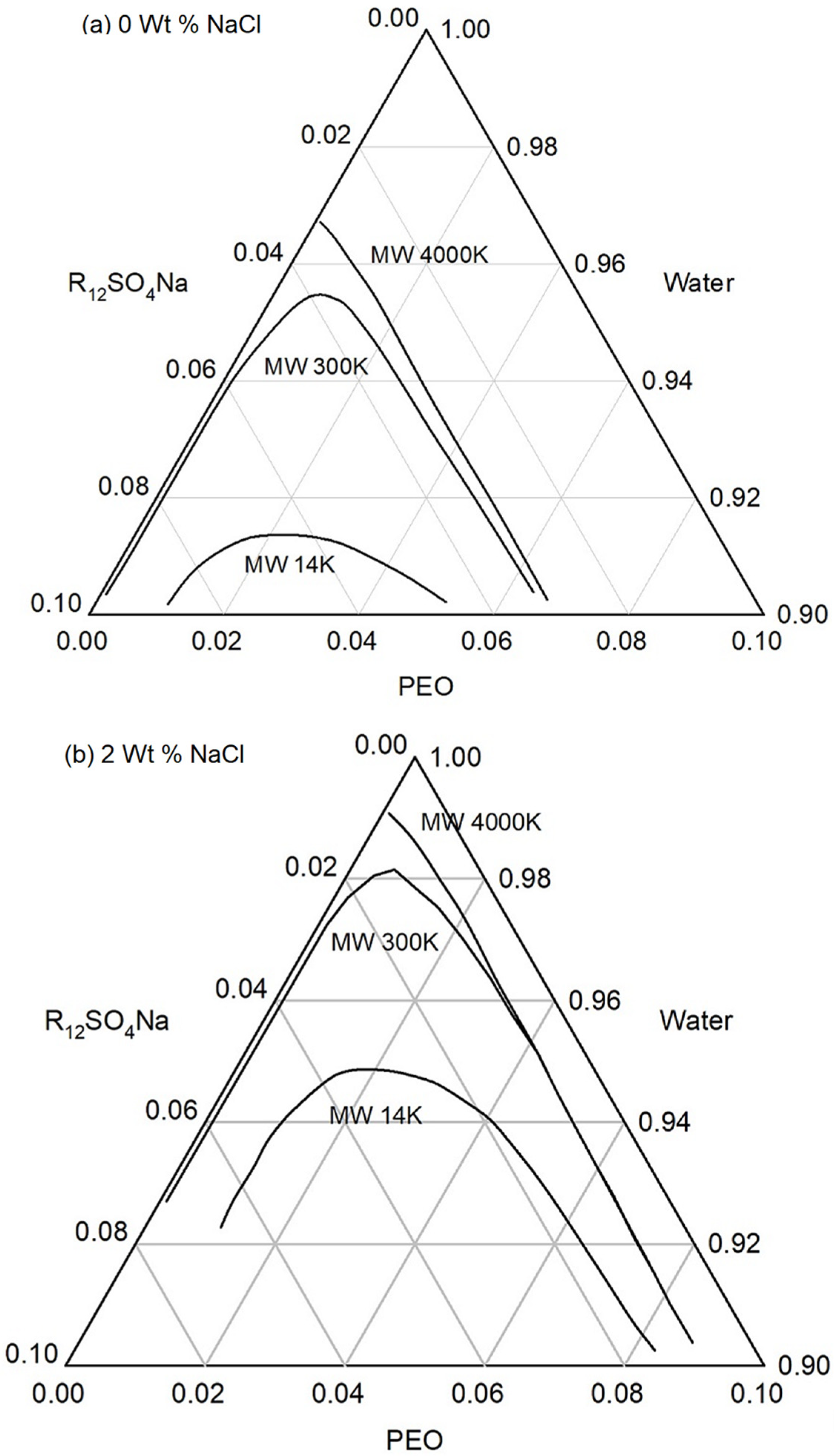
5.2. Construction of Ternary Phase Diagram from Theory Based on iso-ΔG Values

To construct the ternary phase diagram for any polymer–pseudosolvent system, we start from Figure 4, constructed for the polymer of interest (in this case, PEO). For a given polymer molecular weight and concentration, one can determine the value of the characteristic energy parameter ε 1 P * at which phase separation would occur from Figure 4. The corresponding free energy difference ΔG is then determined from Figure 5, which is a universal relation independent of the polymer. All water–surfactant–electrolyte compositions with free energy differing from water by the same magnitude of ΔG will lie at the polymer–pseudosolvent phase boundary, allowing us to construct the phase diagram in the actual compositional space of the polymer + surfactant + electrolyte + water system. These iso-ΔG surfactant + electrolyte + water compositions are determined from Figure 6.
Ternary phase diagrams can thus be constructed in this manner by combining the results for a polymer + water system, such as in Figure 4, obtained from the lattice fluid theory, the universal relation between the characteristic energy of the pseudosolvent and the free energy difference, obtained in the framework of the lattice fluid model shown in Figure 5, and the relation between ΔG and the actual composition of the solution obtained from the polymer-independent models of surfactant + electrolyte systems, as shown in Figure 6. The ternary phase diagrams constructed in the manner are shown in Figure 7 for the polyethylene oxide + sodium dodecyl sulfate + NaCl + water system, at two concentrations of the electrolyte, NaCl.
One can observe the influences of polymer molecular weight, polymer concentration, surfactant concentration, and electrolyte concentration from the ternary diagram. Figure 7a,b both show that increasing surfactant concentration leads to phase separation. Comparing the two figures, we see that increasing the salt concentration reduces the single-phase compositional domain. Similarly, increasing the equivalent weight of the surfactant also decreases the single-phase compositional domain.
In addition to predicting the effects of salt concentration, surfactant concentration, and equivalent weight of surfactant on the phase behavior of the polymer–surfactant solutions in agreement with known experimental behavior, the pseudosolvent model also correctly describes the effect of polymer molecular weight and polymer concentration. Figure 7a,b both show that for high molecular-weight PEO samples, the phase behavior is not changed appreciably by the change in polymer concentration, while for the lower molecular-weight PEO, there is a change with polymer concentration. One can observe that as the polymer concentration is changed, the surfactant concentration at the phase boundary remains practically unchanged in both figures at the given salt concentrations. Both figures show that the compositional space of the single-phase domain is not much altered by the polymer molecular weight, as long as the polymers have high molecular weights.
Both Trushenski et al. [7,8] and Pope et al. [10] found that the influences of polymer concentration (in the range 100 to 1500 ppm) and polymer molecular weight (for molecular weights larger than 400 K) on the phase behavior of the polymer–surfactant–electrolyte systems were negligible. Kalpakci [6] made the same observation and further noted that as the high molecular-weight polymer was degraded using an ultrasonic mixer and/or orifice mixer, the phase stability of the system improved, and the aqueous solution remained stable at higher salt and surfactant concentrations.
Our calculated results in Figure 7 are in agreement with these experimental observations. For the high molecular-weight polymers PEO (4 M) and PEO (300 K) and polymer concentrations in the range of 100 ppm to 1500 ppm (equivalently, 0.01 wt% to 0.15 wt%), the phase behavior is the same, namely, the phase boundaries have the same concentration of the surfactant and electrolyte. In contrast Figure 7 shows that for the lower molecular-weight polymer, PEO (14 K), the concentrations of surfactant and salt at which phase separation would occur are higher. This model prediction is in agreement with the experimental findings of Kalpacki proving that decreasing polymer molecular weight during ultrasonication resulted in enhanced phase stability at higher surfactant and salt concentration.

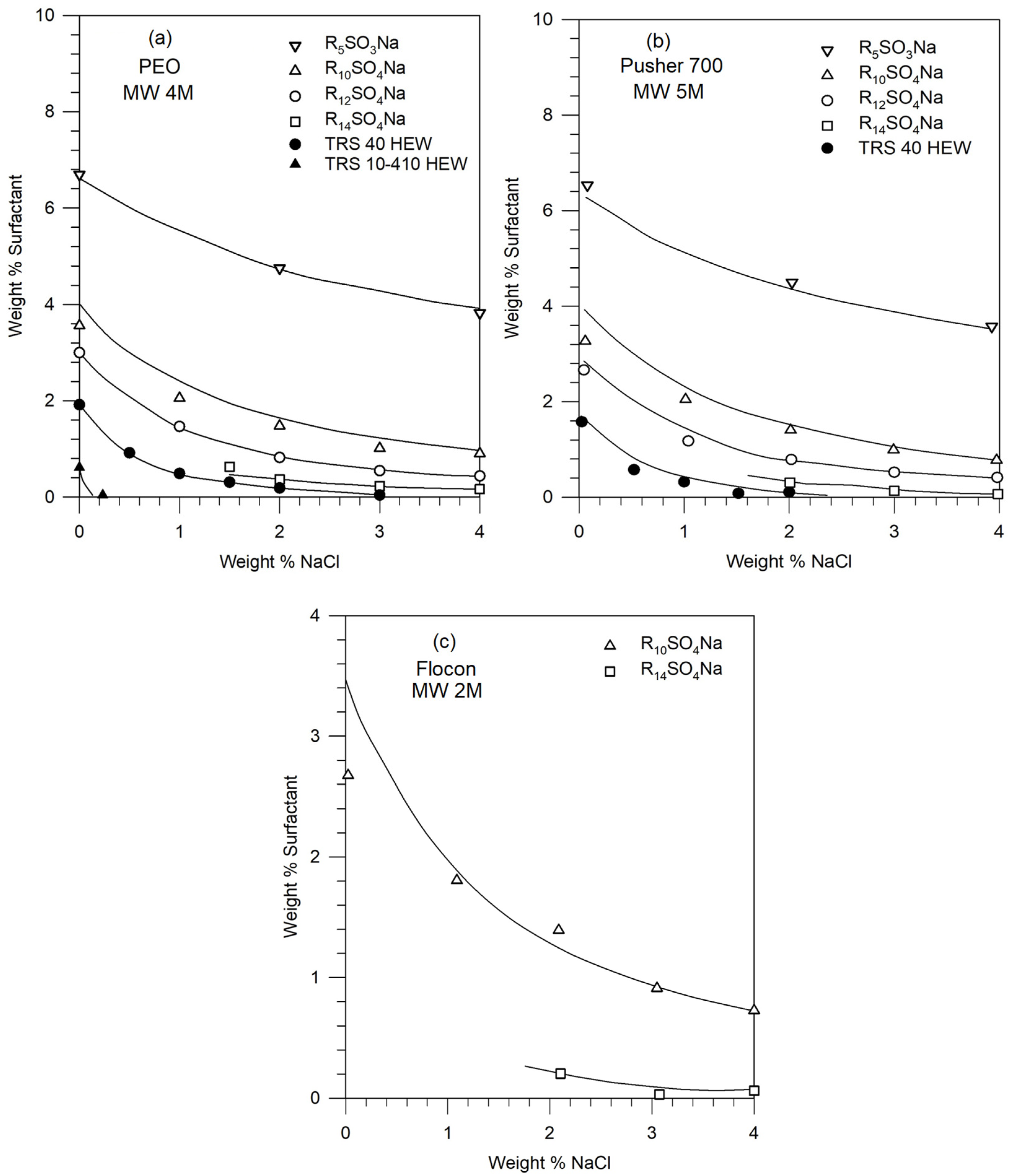
5.3. Construction of Phase Diagram Using a Single Experimental Phase Boundary Data

In the absence of polymer equation-of-state parameters or the binary parameters of the polymer–water system, it will not be possible to calculate a phase diagram similar to Figure 4. In the absence of knowledge of ε 1 P * values, it is not possible to construct a ternary phase diagram such as the one in Figure 7. However, for these situations, we suggest a simple approach to constructing a phase diagram similar to Figure 2. If we know from experiments one composition lying at the phase boundary (any one experimental point in Figure 2), we can calculate the corresponding ΔG of the surfactant + electrolyte + water system from Figure 6 (which can be constructed for that surfactant + electrolyte system). Various combinations of surfactant + electrolyte systems can give rise to identical magnitudes of ΔG (or to identical values of the characteristic energy parameter ε 1 P * ) and are expected to have similar phase behavior in the framework of the pseudosolvent model. All surfactant + electrolyte + water systems having iso-ΔG values can be identified from Figure 6 in order to construct the phase diagram without requiring any information about the polymer. Illustrative phase diagrams calculated in this manner, by using one experimental phase composition data point lying at the phase boundary from Figure 2, are shown in Figure 8 for the three polymers considered in this work.
For example, one of the solution compositions on the phase boundary for the Pusher 700-R12SO4Na system contains 0.76 wt % surfactant and 2.0 wt % NaCl. It can be determined from Figure 6 that the free energy difference ΔG for this pseudosolvent is −33.6 cal/mol. This implies, in the framework of the pseudosolvent model, that all compositions of the pseudosolvent with a free energy difference of −33.6 cal/mol which can be determined from Figure 6 must lie on the phase boundary for the Pusher 700–surfactant–electrolyte system. The iso-ΔG also occurs at 0% NaCl and 2.82 wt% surfactant, and at 4% NaCl and 0.35 wt% surfactant for sodium dodecyl sulfate, providing other compositions lying at the phase boundary. This procedure has been used for the three polymer systems, to establish their predicted phase boundaries, as shown by the continuous lines in Figure 8. The predicted and experimental phase boundaries (shown as points) are found to be in reasonable agreement.
The most significant feature of the pseudosolvent model is thus the possibility of constructing phase diagrams using the knowledge of just one experimental phase composition lying at the phase boundary, and without requiring any information about the polymer. Using this one experimental point, available for any one surfactant and/or electrolyte, one can theoretically establish the phase boundary for the polymer with any other surfactant and electrolyte systems.

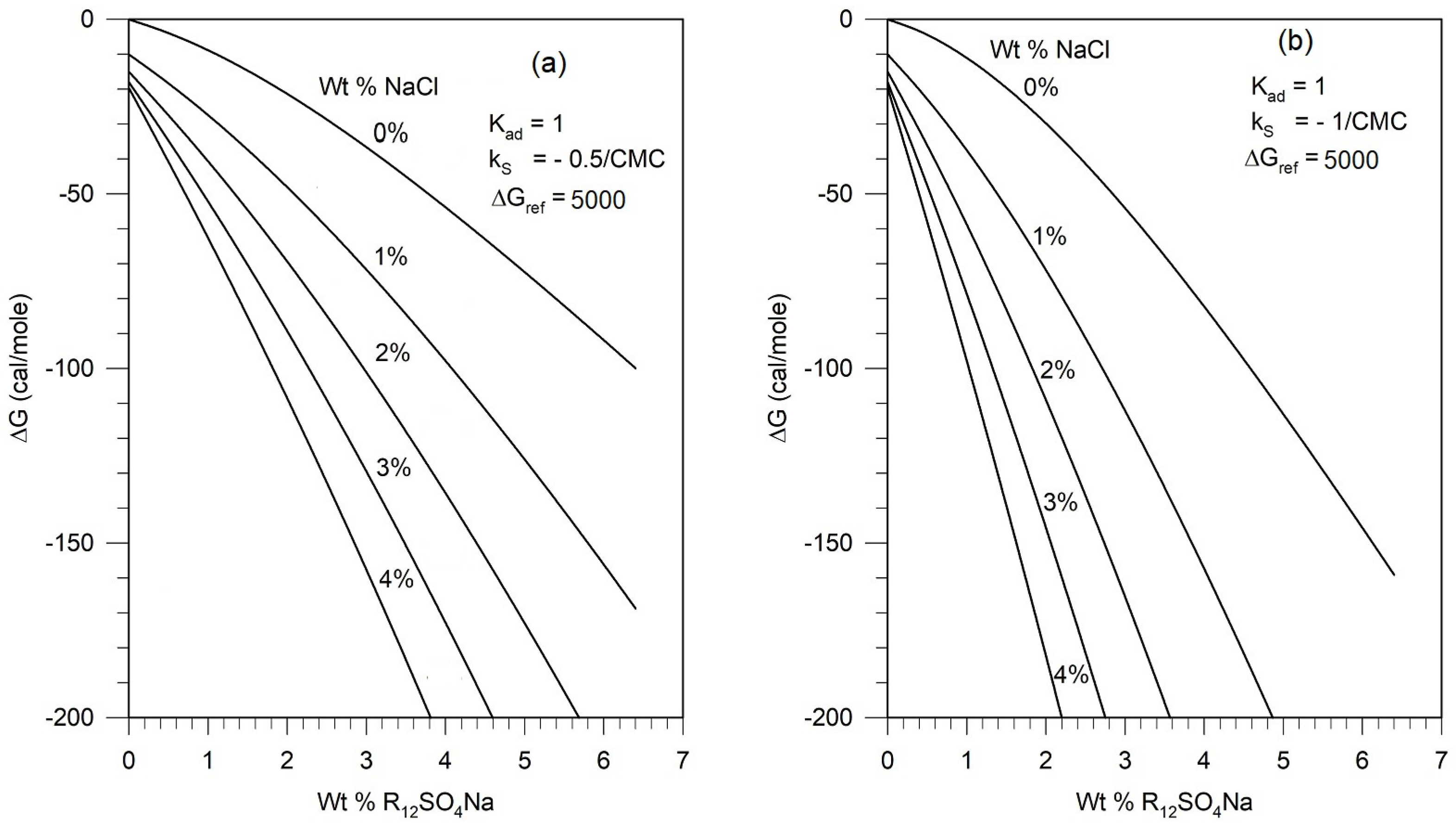
5.4. Assessment of Parametric Sensitivity to Predicted Results

To carry out predictive computations, we have used estimated parameter values where direct experimental data for specific molecules are not available. The choice of values for the degree of dissociation on the micelle surface at an infinite dilution α* and the shielding parameter δ are reasonable, based on available data for multiple surfactants. In contrast, the counterion adsorption equilibrium constant Kad, the Setschenow constant (used to describe the salt effect on surfactant activity) kS, and the correction term ΔGref used to account for the consideration of hydrated ions as the actual species in place of the unhydrated ions have all been assigned values based on limited or no direct experimental data. Therefore, we have performed illustrative calculations to assess the sensitivity of the free energy calculations to variations in these parameter values. The results are shown in Figure 9.
Changes in the values of Kad and kS only change the free energy values to a small extent, and therefore the phase diagrams will change only marginally. The correction term ΔGref does not affect the dependence of the free energy curve on the surfactant concentration, but displaces the curves up or down, that is, to smaller or larger ΔG magnitudes. This will have the effect of shifting the phase boundary curves in Figure 8 up or down. For quantitative comparisons of predictions against experiments, it would be possible to update the present calculations whenever the currently unavailable surfactant parameter values are determined experimentally
The free energy calculations show that the predominant contributions come from the ideal free energy of mixing and the non-ideal free energy contribution arising from the salt effect on the surfactant. All other terms are practically unimportant for the concentrations of salt and surfactant considered in this study, even though they have been rigorously included here. Therefore, improved estimation of the Setschenow constant kS will ensure that true predictions can be obtained.

6. Conclusions

Phase separation in four-component systems made up of polymer + surfactant + electrolyte + water is treated by introducing the concept of a pseudosolvent. This concept transforms the problem to that of a pseudo-binary solution and thus avoids the unmanageability of the thermodynamic description of phase stability criteria in four-component systems. The pseudosolvent is considered to be made up of water, electrolyte, singly dispersed surfactant molecules, and micellar aggregates. The polymer molecule is regarded as the solute. The lattice fluid theory is then used to describe the phase behavior of the polymer + pseudosolvent system. All important characteristics of the pseudosolvent are assumed to be described by a single parameter, namely, the characteristic energy parameter ε 1 P * . This is an extra-thermodynamic postulate underlying the pseudosolvent treatment. This characteristic energy parameter ε 1 P * of the pseudosolvent is related to the free energy difference ΔG between the pseudosolvent and water. In order to calculate the free energy difference ΔG between the pseudosolvent and water, the electrolyte solution theory and surfactant solution theory available in the literature have been used.
The free energy calculations show that the main contributions to the free energy difference ΔG between the pseudosolvent and water come from the ideal free energy of mixing and the non-ideal free energy contribution arising from the salt effect on the surfactant. All other terms are relatively unimportant for the concentrations of salt and surfactant considered in this study. These terms, which have been rigorously modeled in this work, could become important at higher concentrations of electrolytes when studies focus on somewhat smaller polymer molecular weights.
Ternary phase diagrams have been constructed by combining the value of the characteristic energy parameter ε 1 P * at which phase separation would occur, from Figure 4, the polymer-independent universal relation between ε 1 P * and the free energy difference ΔG between the pseudosolvent and water, shown on Figure 5, and the dependence of ΔG on the surfactant–electrolyte composition, shown on Figure 6. The ternary phase diagrams correctly show agreement with the observations in the literature that the phase behaviors of polymer–surfactant solutions show only a slight dependence on the molecular weight of the polymer for high molecular-weight polymers, and they are not very sensitive to polymer concentrations for high molecular-weight polymers at low polymer concentration ranges; the phase stability increases significantly as the polymer’s molecular weight is drastically decreased, and the compositional domain of the single-phase region decreases with increasing polymer molecular weight, increasing surfactant equivalent weight, and added salt concentration.
Most importantly, we present an approach to predict the phase behavior without requiring any information about the polymer, as long as a single experimental composition data point for a system lying on the phase boundary is known. Corresponding to this single composition at the phase boundary, the free energy difference ΔG between the pseudosolvent and water is calculated, using the pseudosolvent model and all model parameters provided. All solution compositions that will lie on the phase boundary are then determined by identifying surfactant–electrolyte compositions having iso-ΔG values. The comparison between the phase boundaries calculated in this manner from the pseudosolvent model and the experimental phase boundaries shows satisfactory agreement. The pseudosolvent model thus offers a predictive approach to determining the phase separation boundary, one which does not depend on any knowledge about the polymer, using information on only a single experimental phase boundary composition.

Author Contributions

Conceptualization, R.N. and J.-Z.S.; experiments, J.-Z.S.; numerical computations, J.-Z.S.; analysis, J.-Z.S. and R.N.; writing—original draft preparation, J.-Z.S. and R.N.; independent numerical computations, R.N.; writing—review and editing, R.N.; supervision, R.N.; project administration, R.N. All authors have read and agreed to the published version of the manuscript.

Funding

This research received no directed external funding.

Data Availability Statement

The original experimental data presented in the study are openly available in Ref. [13]. Other original contributions presented in the study are included in the article and further inquiries can be directed to the corresponding author.

Acknowledgments

Support from The Pennsylvania State University for conducting the research and from the US Army CCDC Soldier Center for preparing the manuscript is gratefully acknowledged.

Conflicts of Interest

The authors declare no conflicts of interest.

Nomenclature

AParameter in the equation for the CMC dependence of on chain length
aParameter in the equation for the CMC dependence on salt concentration
aParameter defined in Equation (A16)
aiActivity of component i
aOH/OH*, aOH*/OHWilson interaction parameters between hydrated water and free water
BParameter in the equation for the CMC dependence of on chain length
bParameter in the equation for the CMC dependence on salt concentration
b12Parameter defined in Equation (A17)
CiMolar concentration of component i
CMCCritical micelle concentration, expressed as molar concentration
c12Parameter defined in Equation (A18)
eElectronic charge (4.8 × 10⁻¹⁰ esu)
GFree energy
G ˜ Reduced free energy
ΔGFree energy difference between pseudosolvent and water
ΔGrefCorrection to free energy change to account for the different reference states for electrolyte ions
IIonic strength of the solution
KadAdsorption equilibrium constant for counterion binding
kBoltzmann constant
kSSetschenow constant
MMolecular weight
MMicelle aggregation number
miMolarity of component i
NChain length of surfactant tail
NNumber of molecules
NiNumber/cm3 concentration of ion i
NoNumber of vacant lattice sites
NAAvogadro number
nNumber of counterions bound to the micelle
nCHydration number of cation
nAHydration number of anion
niNumber of moles of component i
PPressure of system
P ˜ Reduced pressure
P * Characteristic pressure parameter
P i * Characteristic pressure parameter of component i
q k Group fraction of group k
RUniversal gas constant
roIon size parameter in Equation (9)
riNumber of sites occupied by component i
TTemperature of system
T ˜ Reduced temperature
T * Characteristic temperature parameter
T i * Characteristic temperature parameter of component i
VVolume of system
V*Hard-core volume parameter
vVolume per segment
v ˜ Reduced volume
v i * Characteristic lattice site hard-core volume parameter for component i
xiMole fraction of component i
x i h Mole fraction of component i, including water of hydration
X12Variable defined in Equation (A15)
ZiNumber of charges on species i
Greek Letters
αThermal pressure coefficient of polymer
αDegree of counterion dissociation on micelle surface
α*Degree of counterion dissociation on micelle surface at infinite dilution
β Isothermal compressibility of polymer
Γ k Activity coefficient of the interacting group k in the mixture
Γ k ( i ) Standard state activity coefficient of group k
γ i Activity coefficient of component i
γ i FH Activity coefficient of component i due to excess entropic contribution
γ i G Activity coefficient of component i due to enthalpic contribution
γ i S Activity coefficient contribution due to surfactant for component i
γ ± S S Average activity coefficient of surfactant
γ i FH Total number of fundamental groups in species i
δPolymer–solvent binary volume parameter correcting deviation from arithmetic mean
δ Shielding parameter for micelle surface charge
ε Dielectric constant of water
ε 1 * Characteristic energy parameter of solvent (water)
ε 1 P * Characteristic energy parameter of pseudosolvent
ε 2 * Characteristic energy parameter of polymer
κInverse Debye length defined in Equation (9)
μ 1 Chemical potential of component 1
νRatio of characteristic hard-core volumes appearing in Equation (A16)
ν i Number of atoms other than H in component i
ν ki Number of interacting groups of kind k in component i
ξPolymer–solvent binary energy parameter correcting deviation from geometric mean
ρDensity
ρ ˜ Reduced density
ρ * Characteristic density parameter
τRatio of characteristic energies appearing in Equation (A16)
φ i Volume fraction of component i
χ 12 Interaction parameter defined by Equation (A14)
ψParameter defined by Equation (A22)
ωMolecular constant associated with molecular size and flexibility
Superscripts
hHydration
Infinite dilution
Subscripts
1Water
2Polymer while discussing polymer–solvent systems
2Counterion of electrolyte
3Co-ion of electrolyte
4Counterion of surfactant
4SCounterion of free (singly dispersed) surfactant
5Co-ion of surfactant
5SCo-ion of free (singly dispersed) surfactant
AAnion including associated hydrated water
CCation including associated hydrated water
iComponent i
micMicelle
wFree water

Appendix A. Lattice Fluid Theory

Appendix A.1. Equation of State for Pure Fluids

The lattice fluid theory developed by Sanchez [9,10,11,12,13] differs from other lattice models in the literature such as the Flory–Prigogine equation-of-state model, by allowing for some of the lattice sites to be vacant. For a system consisting of N molecules, each of which occupies r sites (a r-mer) and No vacant lattice sites (holes), the reduced Gibbs energy is given by
G ˜ = G N r ε * = ρ ˜ + P ˜ v ˜ + T ˜ [ ( v ˜ 1 ) ln ( 1 ρ ) ˜ + 1 r ln ( ρ ˜ / ω ) ]
where the reduced variables are defined as
P ˜ = P / P * , T ˜ = T / T * , v ˜ = 1 / ρ ˜ = V / V * ; T * = ε * / k , P * = ε * / v * , V * = rv *
and ω is a molecular constant associated with molecular size and flexibility, while k is the Boltzmann constant. The corresponding equation of state for a pure fluid is obtained from the condition
( G ˜ / v ˜ ) T ˜ , P ˜ = 0
and is given by
ρ ˜ 2 + P ˜ + T ˜ [ ln ( 1 ρ ) ˜ + ( 1 1 r ) ρ ˜ ] = 0
The equation-of-state parameters can be the characteristic pressure P*, characteristic temperature T*, and the characteristic volume V*, or, alternately, the characteristic energy ε*, the characteristic lattice size v*, and the component molecular size r.

Appendix A.2. Estimation of Equation-of-State Parameters

The lattice fluid theory is applicable to liquid and gas phases. Therefore, the equation-of-state parameters for pure fluids can be estimated by using experimental liquid phase P-V-T data or by using the saturation vapor pressure data. By fitting available vapor pressure data to the equation of state, Equation (A4), Sanchez obtained the equation-of-state parameters for water (the solvent is designated by subscript 1):
P 1 * = 26.520 atm , T 1 * = 623 ° K , ρ 1 * = 1.105 g / cm 3 ε 1 * = 1.238 kcal / mol , v 1 * = 1.93 cm 3 / mol , r 1 = 8.46
For polymers, vapor pressure data are not generally available, since high molecular-weight polymers have negligible vapor pressures. Therefore the equation-of-state parameters are usually determined by fitting the experimental density data above the glass transition temperature to the equation of state. An alternate approach is to use information available at a single temperature for the density ρ, thermal expansion coefficient α, and the isothermal compressibility β. From the equation of state, one can get expressions for α and β as follows:
α = lnV T P , T α = 1 + P ˜ v ˜ 2 T ˜ v ˜ [ 1 / ( v ˜ 1 ) + 1 / r ] 2 β = lnV P T , P β = P ˜ v ˜ 2 T ˜ v ˜ [ 1 / ( v ˜ 1 ) + 1 / r ] 2
For high molecular-weight polymers ( r ) and at atmospheric pressure ( P 0 ), the equation of state and the expressions for α and β reduce to
ρ ˜ 2 + T ˜ [ ln ( 1 ρ ) ˜ + ρ ˜ ] = 0 T α = 1 T ˜ / ( 1 ρ ˜ ) 2 , P * β = v ˜ 2 T ˜ / ( 1 ρ ˜ ) 2 = T α ρ ˜ 2
We start with experimental data for ρ, α, and β, available at one temperature. By fitting them to Equation (A7), the equation-of-state parameters for the polymer can be estimated. Using available data for ρ, α, and β at 25 °C, we determine the equation-of-state parameters for PEO to be
P 2 * = 3963 atm , T 2 * = 597 ° K , ρ 2 * = 1.202 g / cm 3 ε 2 * = 1.194 kcal / mol , v 2 * = 12.36 cm 3 / mol , r 2 = M 2 / ( ρ 2 * v 2 * )
Note that r2 is obviously dependent on the molecular weight M2 of the polymer, as shown in Equation (A8).

Appendix A.3. Equation of State for Polymer Solution

In the framework of the lattice fluid theory, the reduced Gibbs energy of a polymer solution is given by
G ˜ = G N r ε * = ρ ˜ + P ˜ v ˜ + T ˜ [ ( v ˜ 1 ) ln ( 1 ρ ˜ ) + 1 r ln ( ρ ˜ ) ] + i φ i r i ln ( φ i / ω i )
where ω i is a molecular constant associated with molecular size and flexibility for component i, and is independent of the composition. In Equation (A9), combining rules are invoked to describe the interaction energy, the close-packed volume per lattice site, and the characteristic molecular size r as a function of the mixture composition, represented by the volume fraction φ i . Denoting the volume fractions of the solvent and the polymer by φ 1 and φ 2 , respectively, the following combining rules are adopted:
v * = i j φ i φ j v ij * = φ 1 v 1 * + φ 2 v 2 * + φ 1 φ 2 δ ( v 1 * + v 2 * ) ε * = i j φ i φ j v ij * ε ij * / v * = φ 1 2 v 1 * ε 1 * + φ 2 2 v 2 * ε 2 * + φ 1 φ 2 ( 1 + δ ) ( v 1 * + v 2 * ) ξ ( ε 1 * ε 2 * ) 1 / 2 v * r = φ 1 r 1 + φ 2 r 2 1
Two binary parameters ξ and δ have been introduced to represent deviations from the “ideal” behavior of the dissimilar lattice occupants.
v 12 * = ( v 1 * + v 2 * ) 2 ( 1 + δ ) , δ = 0 for ideal mixture ε 12 * = ξ ( ε 1 * ε 2 * ) 1 / 2 , ξ = 1 for ideal mixture
The corresponding equation of state for the polymer solution (polymer–solvent mixture) has a form identical to that for pure fluids, and is given by
ρ ˜ 2 + P ˜ + T ˜ [ ln ( 1 ρ ) ˜ + ( 1 1 r ) ρ ˜ ] = 0

Appendix A.4. Estimation of Binary Parameters by Fitting Water Activity

The binary parameters ξ and δ are determined by fitting relevant experimental data for mixtures, such as the activity or the heat and volume changes, on the mixing data. Since we are interested in phase behavior, we use the solvent (water) activity data to estimate the binary parameters. The activity of the solvent is derived from the mixture free energy and is given by
μ 1 kT = ln φ 1 + ( 1 r 1 r 2 ) φ 2 + r 1 χ 12 φ 2 2
where χ 12 is given by
χ 12 = ρ ˜ X 12 kT + P ˜ 1 v ˜ T ˜ 1 ( 1 + 1 ρ ˜ ) δ + 1 T ˜ 1 φ 2 2 ρ ˜ + P ˜ 1 v ˜ + T ˜ 1 v ˜ [ ( 1 ρ ˜ ) ln ( 1 ρ ˜ ) + ρ ˜ r 1 ln ( ρ ˜ ) ]
For a liquid mixture at atmospheric pressure, the two pressure terms in Equation (A14) can be ignored. The variable X 12 is calculated as follows:
X 12 = ( P 1 * P 2 * ) 1 / 2 v 1 * v 2 * v * 2 [ a + b 12 δ + c 12 δ 2 ]
a = ( τ ν ) 1 / 2 + ( ν τ ) 1 / 2 ξ ( ν 1 / 2 + ν 1 / 2 ) , τ = ε 1 * ε 2 * , ν = v 1 * v 2 *
b 12 = [ φ 1 ( 2 + ν φ 1 ) ( τ 1 / 2 ξ ) φ 2 2 ( ξ τ 1 / 2 ) ] ( ν 1 / 2 + ν 1 / 2 )
c 12 = φ 1 2 ( τ 1 / 2 ξ ) ( 1 + ν ) ( ν 1 / 2 + ν 1 / 2 )
All of the solvent (water) and polymer (PEO) pure component parameters have already been estimated, as described in Appendix A.2. By fitting the water activity data to Equations (A13)–(A18), the two unknown binary parameters are determined to be ξ = 1.023 and δ = −0.25 for the PEO–water binary mixture.

Appendix A.5. Criteria for Phase Stability

At constant temperature and pressure, a necessary and sufficient condition for miscibility of a binary mixture over the entire composition range is for the Gibbs free energy per mole of the mixture to be a convex function of composition, i.e.,
d 2 G d φ 1 2 > 0
This condition guarantees that the free energy of mixing is negative. The criteria for the mixture to be stable has been derived by Sanchez as
1 2 1 r 1 φ 1 + 1 r 2 φ 2 ρ ˜ X + 1 2 ψ 2 T ˜ P * β > 0
where
ρ ˜ X = 1 2 ρ ˜ kT 2 ( φ 1 X 21 + φ 2 X 12 ) + φ 1 2 dX 21 d φ 1 φ 2 2 dX 12 d φ 1 + P ˜ v ˜ T ˜ v * δ ( v 1 * + v 2 * )
ψ = ρ ˜ 1 T ˜ 1 1 T ˜ 2 + 1 kT ( φ 1 2 X 21 φ 2 2 X 12 ) + P ˜ v ˜ T ˜ v * ( v 1 * v 2 * ) + ( v 1 * + v 2 * ) ( φ 2 φ 1 ) δ 1 r 1 1 r 2
T ˜ P * β = v ˜ ρ ˜ 1 ρ ˜ + 1 r 2 ρ ˜ T ˜ 1
The expression for X21 appearing in Equations (A21) and (A23) is obtained by interchange of the indices 1 and 2 in Equations (A14)–(A17) for X12. Given the equation-of-state parameters for the polymer (PEO) and two of the equation-of-state parameters for the pseudosolvent (taken to be the same for water), as well as the binary parameters (taken to be the same as for polymer–water), one can numerically solve Equations (A14)–(A23) to determine the characteristic energy parameter for the pseudosolvent when the stability criteria, Equation (A20), is met, for any given polymer molecular weight and polymer concentration (volume or weight fraction). The calculations are repeated for various concentrations of the polymer, and the results are shown in Figure 4 of the main text. The calculations are also repeated for polymers of different molecular weights, and the corresponding results are plotted in the same figure.

References

  1. Hansson, P.; Lindman, B. Surfactant-polymer interactions. Curr. Opin. Colloid Interface Sci. 1996, 1, 604–613. [Google Scholar] [CrossRef]
  2. Shah, D.O.; Schechter, R.S. (Eds.) Improved Oil Recovery by Surfactant and Polymer Flooding; Academic Press: New York, NY, USA, 1977. [Google Scholar]
  3. Druetta, P.; Picchioni, F. Surfactant–Polymer Flooding: Influence of the Injection Scheme. Energy Fuels 2018, 32, 12231–12246. [Google Scholar] [CrossRef]
  4. Druetta, P.; Picchioni, F. Surfactant-Polymer Interactions in a Combined Enhanced Oil Recovery Flooding. Energies 2020, 13, 6520. [Google Scholar] [CrossRef]
  5. Hamouma, M.; Delbos, A.; Dalmazzone, C.; Colin, A. Polymer Surfactant Interactions in Oil Enhanced Recovery Processes. Energy Fuels 2021, 35, 9312–9321. [Google Scholar] [CrossRef]
  6. Gradzielski, M. Polymer–surfactant interaction for controlling the rheological properties of aqueous surfactant solutions. Curr. Opin. Colloid Interface Sci. 2023, 63, 101662. [Google Scholar] [CrossRef]
  7. Trushenski, S.P.; Dauber, D.L.; Parris, D.R. Micellar Flooding—Fluid Propagation, Interaction, and Mobility. Soc. Pet. Eng. J. 1974, 14, 633–645. [Google Scholar] [CrossRef]
  8. Trushenski, S.P. Micellar Flooding: Sulfonate-Polymer Interaction. In Improved Oil Recovery by Surfactant and Polymer Flooding; Shah, D.O., Schechter, R.S., Eds.; Academic Press: New York, NY, USA, 1977; pp. 555–575. [Google Scholar]
  9. Szabo, M.T. The Effect of Sulfonate/Polymer Interaction on Mobility Buffer Design. Soc. Pet. Eng. J. 1979, 19, 5–14. [Google Scholar] [CrossRef]
  10. Pope, G.A.; Tsaur, K.; Schecter, R.S.; Wang, B. Effect of Several Polymers on the Phase Behavior of Micellar Fluids. Soc. Pet. Eng. J. 1982, 22, 816–830. [Google Scholar] [CrossRef]
  11. Gupta, S.P. Dispersive Mixing Effects on the Sloss Field Micellar System. SPE J. 1982, 22, 481–492. [Google Scholar] [CrossRef]
  12. Kalpakci, B. Flow Properties of Surfactant Solution in Porous Media and Surfactant-Polymer Interactions. Ph.D. Thesis, Department of Chemical Engineering, The Pennsylvania State University, University Park, PA, USA, 1981. [Google Scholar]
  13. Sheu, J.-Z. Thermodynamics of Phase Separation in Aqueous Polymer-Surfactant-Electrolyte Solution. Ph.D. Thesis, Department of Chemical Engineering, The Pennsylvania State University, University Park, PA, USA, 1983. [Google Scholar]
  14. Flory, P.J. Principles of Polymer Chemistry; Cornell University Press: Ithaca, NY, USA, 1953. [Google Scholar]
  15. Dormidontova, E.E. Role of Competitive PEO-Water and Water-Water Hydrogen Bonding in Aqueous Solution PEO Behavior. Macromolecules 2002, 35, 987–1001. [Google Scholar] [CrossRef]
  16. Knychala, P.; Timachova, K.; Banaszak, M.; Balsara, N.P. 50th Anniversary Perspective: Phase Behavior of Polymer Solutions and Blends. Macromolecules 2017, 50, 3051–3065. [Google Scholar] [CrossRef]
  17. Mkandawire, W.D.; Milner, S.T. Simulated Osmotic Equation of State for Poly(ethylene Oxide) Solutions Predicts Tension—Induced Phase Separation. Macromolecules 2021, 54, 3613–3619. [Google Scholar] [CrossRef]
  18. Bekiranov, S.; Bruinsma, R.; Pincus, P. Solution behavior of polyethylene oxide in water as a function of temperature and pressure. Phys. Rev. E 1996, 55, 577–585. [Google Scholar] [CrossRef]
  19. Valsecchia, M.; Galindo, A.; Jackson, G. Modelling the thermodynamic properties of the mixture of water and polyethylene glycol (PEG) with the SAFT-γ Mie group-contribution approach. Fluid Phase Equilibria 2024, 577, 113952. [Google Scholar] [CrossRef]
  20. Sanchez, I.C.; Lacombe, R.H. An elementary molecular theory of classical fluids. Pure fluids. J. Phys. Chem. 1976, 80, 2352–2362. [Google Scholar] [CrossRef]
  21. Lacombe, R.H.; Sanchez, I.C. Statistical thermodynamics of fluid mixtures. J. Phys. Chem. 1976, 80, 2568–2580. [Google Scholar] [CrossRef]
  22. Sanchez, I.C.; Lacombe, R.H. An elementary equation of state for polymer liquids. J. Polym. Sci. Polym. Lett. Ed. 1977, 15, 71–75. [Google Scholar] [CrossRef]
  23. Sanchez, I.C.; Lacombe, R.H. Statistical thermodynamics of polymer solutions. Macromolecules 1978, 11, 1145–1156. [Google Scholar] [CrossRef]
  24. Sanchez, I.C. Statistical thermodynamics of bulk and surface properties of polymer mixtures. J. Macromol. Sci. Phys. 1980, 17 Pt B, 565–589. [Google Scholar] [CrossRef]
  25. Panayiotou, C.; Sanchez, I.C. Hydrogen Bonding in Fluids: An Equation-of-State Approach. J. Phys. Chem. 1991, 95, 10090–10097. [Google Scholar] [CrossRef]
  26. Malcolm, G.N.; Rowlinson, J.S. The thermodynamic properties of aqueous solutions of polyethylene glycol, polypropylene glycol and dioxane. Trans. Faraday Soc. 1957, 53, 921–931. [Google Scholar] [CrossRef]
  27. Kawaguchi, Y.; Kanai, H.; Kajiwara, H.; Arai, Y.J. Correlation for Activities of Water in Aqueous Electrolyte Solutions Using ASOG Model. J. Chem. Eng. Jpn. 1981, 14, 243–246. [Google Scholar] [CrossRef]
  28. Ronc, M.; Ratcliff, G.A. Prediction of excess free energies of liquid mixtures by an analytical group solution model. Can. J. Chem. Eng. 1971, 49, 825–830. [Google Scholar] [CrossRef]
  29. Wilson, G.M. Vapor-Liquid Equilibrium. XI. A New Expression for the Excess Free Energy of Mixing. J. Am. Chem. Soc. 1964, 86, 127–130. [Google Scholar] [CrossRef]
  30. Kojima, K.; Tochigi, K. Prediction of Vapor-Liquid Equilibria by the ASOG Method; Kodansha Ltd.: Tokyo, Japan, 1979. [Google Scholar]
  31. Robinson, R.A.; Stokes, R.H. Electrolyte Solutions, 2nd ed.; Butterworths: London, UK, 1965. [Google Scholar]
  32. Fowler, R.H.; Guggenheim, E.A. Statistical Thermodynamics; Cambridge University Press: Cambridge, UK, 1949; Chapter IX. [Google Scholar]
  33. Rosen, M.J. Surfactants and Interfacial Phenomena, 3rd ed.; Wiley-Interscience: New York, NY, USA, 2004. [Google Scholar]
  34. Burchfield, T.E.; Woolley, E.M. Model for Thermodynamics of Ionic Surfactant Solutions. 1. Osmotic and Activity Coefficients. J. Phys. Chem. 1984, 88, 2149–2155. [Google Scholar] [CrossRef]
  35. Dauheret, G.; Viallard, A. Activity Coefficients and Micellar Equilibria. I. The Mass Action Law Model Applied to Aqueous Solutions of Sodium Carboxylates at 298.15 K. Fluid Phase Equilibria 1982, 8, 233–250. [Google Scholar] [CrossRef]
  36. Long, F.A.; McDevit, W.F. Activity Coefficients of Nonelectrolyte Solutes in Aqueous Salt Solutions. Chem. Rev. 1952, 51, 119–169. [Google Scholar] [CrossRef]
  37. Setschenow, J. Über die Konstitution der Salzlösungen auf Grund ihres Verhaltens zu Kohlensäure. Z. Physik. Chem. 1889, 4, 117–125. [Google Scholar] [CrossRef]
  38. Deno, N.C.; Spink, C.H. The McDevit-Long equation for salt effects on non-electrolytes. J. Phys. Chem. 1963, 67, 1347–1349. [Google Scholar] [CrossRef]
  39. Mukerjee, P. Salt Effects on Nonionic Association Colloids. J. Phys. Chem. 1965, 69, 4038–4040. [Google Scholar] [CrossRef]
  40. Hall, D.G.; Tiddy, G.J.T. Surfactant Solutions: Dilute and Concentrated. In Anionic Surfactants. Physical Chemistry of Surfactant Action; Lucassen-Reynders, E.H., Ed.; Marcel Dekker: New York, NY, USA, 1981; Chapter 2. [Google Scholar]
  41. Corrin, M.L.; Harkins, W.D. The effect of salts on the critical concentration for the formation of micelles in colloidal electrolytes. J. Am. Chem. Soc. 1947, 69, 683–688. [Google Scholar] [CrossRef] [PubMed]
  42. Rosenholm, J.B. Critical evaluation of models for self-assembly of short and medium chain-length surfactants in aqueous solutions. Adv. Colloid Interface Sci. 2020, 276, 102047. [Google Scholar] [CrossRef] [PubMed]
  43. MacNeil, J.A.; Ray, G.B.; Sharma, P.; Leaist, D.G. Activity Coefficients of Aqueous Mixed Ionic Surfactant Solutions from Osmometry. J. Solut. Chem. 2014, 43, 93–108. [Google Scholar] [CrossRef]
Figure 1. Molecular structures of the polymers and surfactants used in this study. The polymers include xanthan with pentasaccharide repeat unit, partially hydrolyzed polyacrylamide, and polyethyleneoxide. The surfactants include sodium alkyl sulfates and sodium alkyl benzene sulfonates, with the alkyl benzene sulfonates denoting petroleum sulfonates.
Colloids 08 00040 g001
Figure 2. Experimental phase boundaries at 25 °C in solutions containing 1500 ppm polymer, anionic sulfate or sulfonate-type surfactants, and the electrolyte NaCl. Phase behavior data for (a) the nonionic polymer PEO (MW 4 M), (b) the anionic polymer Pusher 700 (MW 5 M), and (c) the anionic biopolymer Flocon (MW 2 M) are shown.
Colloids 08 00040 g002
Figure 3. Experimental water activity data [26] at 65 °C in solutions containing 1500 ppm polyethylene oxide; MW (circles) fitted to the activity calculated from the lattice fluid theory for polymer solutions (line).
Colloids 08 00040 g003
Figure 4. Theoretical phase boundaries of nonionic polymer PEO and various pseudosolvents of characteristic energy parameter ε 1 P * at 1 atm and 25 °C. The different lines correspond to polymer molecular weights of 14 K, 300 K, and 4 M, respectively. Regions below the curves are single-phase and those above correspond to two phases.
Colloids 08 00040 g004
Figure 5. The relationship between the free energy difference ΔG between the pseudosolvent and water and the characteristic energy parameter ε 1 P * of the pseudosolvent.
Colloids 08 00040 g005
Figure 6. Free energy difference ΔG between the pseudosolvent and water as a function of surfactant and electrolyte (sodium chloride) concentrations at 25 °C for (a) sodium pentyl sulfonate (CH3(CH2)4SO3Na), (b) sodium dodecyl sulfate (CH3(CH2)11SO4Na), and (c) TRS 40 (CH3(CH2)10C6H4SO3Na).
Colloids 08 00040 g006
Figure 7. Ternary phase diagram of the system, consisting of the nonionic polymer PEO, water, anionic surfactant R12SO4Na at (a) 0% NaCl and (b) 2% NaCl, at 25 °C. The phase boundaries are shown for three different molecular weights of the polymer. The domains under the phase boundaries are two-phase regions, and those above the boundaries are single-phase regions.
Colloids 08 00040 g007
Figure 8. Predicted phase boundaries at 25 °C in solutions containing 1500 ppm polymer and anionic alkyl sulfate or alkyl sulfonate type surfactants, in the presence of NaCl as the electrolyte. The plots correspond to (a) the nonionic polymer, PEO (MW 4 M); (b) the anionic polymer, Pusher 700 (5 M); and (c) the anionic biopolymer, Flocon (2 M). The experimental phase boundaries are denoted by the points and the predicted phase boundaries are shown as continuous lines. A single experimental data point for a given polymer is taken to estimate ΔG and used to construct all the predictive curves.
Colloids 08 00040 g008
Figure 9. Parametric sensitivity of the free energy calculations. (a) refers to parameter values employed in this paper for the phase behavior calculations. In (b), the Setschenow constant kS for the salt effect on the surfactant is modified. In (c), the equilibrium constant Kad, used for counterion binding on the micelle surface, is modified. In (d), the reference free energy correction term ΔGref, used to account for the difference between the hydrated and unhydrated state of the ions is modified.
Colloids 08 00040 g009aColloids 08 00040 g009b
Table 1. Water-soluble polymers used in the experimental study.
PolymerMWCommercial
Name
Supplier
Partially hydrolyzed Polyacrylamide 5 × 10⁶Pusher 700Dow Chemical Co.
Polyethylene oxide4 × 106PEOBDH Chemical Ltd.
Biopolymer Xanthan2 × 106FloconPfizer Chemical
Table 2. Commercial surfactants used in the experimental study.
SurfactantStructureEqWtSupplier
Sodium pentylsulfonateCH3(CH2)4SO3Na174Fisher Scientific
Sodium decyl sulfateCH3(CH2)9SO4Na260Pfaltz & Bauer
Sodium dodecylsulfateCH3(CH2)11SO4Na288BDH Chemical
Sodium tetradecylsulfateCH3(CH2)13SO4Na316Pfaltz & Bauer
TRS 40 HEWCH3(CH2)10C6H4SO3Na334Witco Chemical
TRS 10-410 HEWCH3(CH2)17C6H4SO3Na436Witco Chemical
Table 3. Hydration numbers of ions.
IonHydration Number
Li+1.8
Na+1.0
K+0.4
Mg2+3.6
Ba2+1.9
Ca2+3.1
Ni2+3.2
Fe2+3.1
I1.0
Br0.8
Cl0.5
Disclaimer/Publisher’s Note: The statements, opinions and data contained in all publications are solely those of the individual author(s) and contributor(s) and not of MDPI and/or the editor(s). MDPI and/or the editor(s) disclaim responsibility for any injury to people or property resulting from any ideas, methods, instructions or products referred to in the content.

