Theoretical Principles and Perspectives of Hyperspectral Imaging Applied to Sediment Core Analysis

Abstract

Hyperspectral imaging is a recent technology that has been gaining popularity in the geosciences since the 1990s, both in remote sensing and in the field or laboratory. Indeed, it allows the rapid acquisition of a large amount of data that are spatialized on the studied object with a low-cost, compact, and automatable sensor. This practical article aims to present the current state of knowledge on the use of hyperspectral imaging for sediment core analysis (core logging). To use the full potential of this type of sensor, many points must be considered and will be discussed to obtain reliable and quality data to extract many environmental properties of sediment cores. Hyperspectral imaging is used in many fields (e.g., remote sensing, geosciences and artificial intelligence) and offers many possibilities. The applications of the literature will be reviewed under five themes: lake and water body trophic status, source-to-sink approaches, organic matter and mineralogy studies, and sedimentary deposit characterization. Afterward, discussions will be focused on a multisensor core logger, data management, integrated use of these data for the selection of sample areas, and other opportunities. Through this practical article, we emphasize that hyperspectral imaging applied to sediment cores is still an emerging tool and shows many possibilities for refining the understanding of environmental processes.

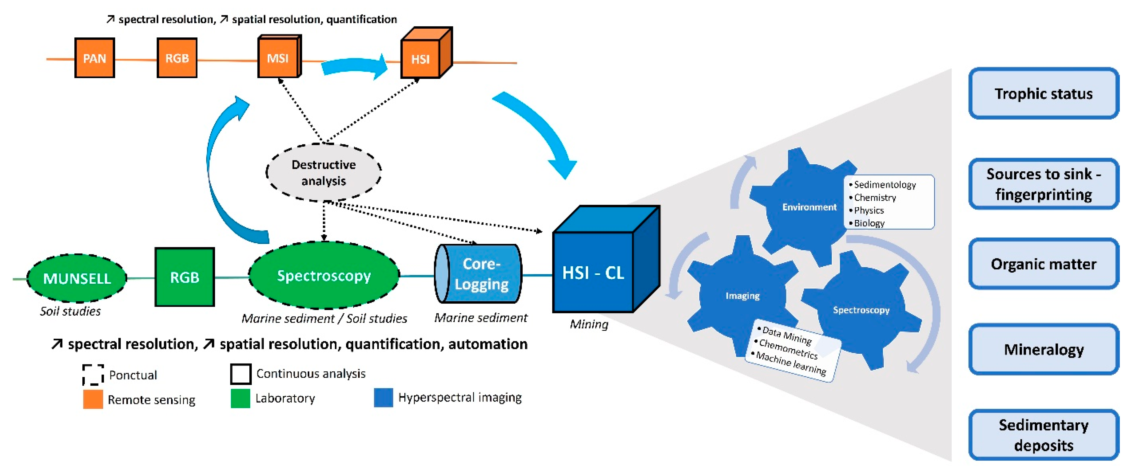
1. Why Develop a New Sensor for Sediment Color Analysis?

The color analysis of sediment in the laboratory has followed important technological developments in closely related fields, such as the analysis of soils and sedimentary rocks, as well as in more distant fields, such as remote sensing. This has led to the development of sensors allowing the analysis of color and, more generally, of the electromagnetic spectrum of light to answer problems of rapidity, high resolution, automation, and increasing the amount of interesting information remotely without affecting the sample. The hyperspectral imaging sensor will be the focus of this practical guide. In the following paragraphs, the different steps that led to the use of hyperspectral imaging in the geosciences, the different fields involved in these developments, and their exploitation will be discussed (Figure 1).

1.1. Munsell Lithology Description

Color and texture are two simple and important parameters to describe sediment facies. However, they are qualitative, and they lack rules to compare several sequences between them. This is why the soil community has adopted the work of Albert Henry Munsell on color classification [1] to standardize the characterization of sample colors. This approach was then adapted for use onboard Ocean Drilling Program (ODP) coring ships such as the JOIDES Resolution and the Marion Dufresne [2,3]. Then, it was democratized in various sedimentological studies.

The Munsell color chart is based on our vision with characterization of sediment color thanks to the definition of three parameters: hue (the color), value (its intensity), and chroma (its brightness). It is also the basis of some color spaces for digital object vision (Lab) [4].

However, this method has limitations, as it is dependent on the experimenter’s vision and the lighting conditions, and the procedure can be time-consuming. It provides information on the sediment color at a given time to reveal development of structures, which change with the oxidation process as well as moisture content [5].

1.2. RGB Imaging

To overcome the subjective nature of visual observations, it is necessary to use reproducible and quantitative approaches. This is why the use of sensors recording colors has received great interest to archive the primary information of the sample (e.g., color and texture) before its destruction. The first imaging sensors are used to save the information in grayscale [6,7,8,9] or X-ray [10], but the interpretation of these levels is complex, as many mixtures of compounds may be involved. This is why RGB (red, green, blue) imaging is currently used because it provides information on three types of colors [11,12].

Image sensors allow a resolution finer than the human eye and thus characterize finer variations. Moreover, the use of image processing can be applied to sediment cores to characterize different deposits, which allows us to complement the experimenter’s vision [11,13,14,15,16,17]. These images also allow us to observe temporal transformations on sample surfaces and to incorporate laboratory results so that we can have better constraints of stratigraphic positions for the analyzed data points. Even if their use is widespread, these images are rarely processed to extract the maximum amount of information (deposits, particle size distribution, etc.), and these three channels as well as the grayscale levels do not allow a precise characterization of compounds within sediment.

1.3. Spectroscopic Analysis

RGB imaging, similar to our eyes, is sensitive to three wavelength zones (610 nm, 550 nm, and 466 nm), while the entire electromagnetic spectrum (Figure 2) provides more information on the sample properties. The development of spectroscopic sensors such as spectrophotometry has allowed more accurate quantification of color through the different wavelengths they record (400–700 nm) directly. Moreover, their simplicity of use, speed, and cost have allowed their democratization. These sensors were used routinely during oceanic campaigns [6,18,19,20,21] and then for the characterization of rocks [22] before their use in the various disciplines of sedimentology [23,24,25]. Spectrophotometric spectra are now commonly used to estimate the total reflectance L* to correlate cores, some minerals and organic pigments [20,21,22,26,27,28,29]. The improvement of the detectors has allowed us to extend the spectral range to cover visible and near-infrared wavelengths (400–2500 nm), which allows us to obtain information on pigments and organic and mineral matter [30,31,32].

Please check that the intended meaning is retained.

Other sensors have also been developed to characterize other spectral ranges that allow us to characterize more sedimentary properties (Figure 2). XRF core logging is currently a very often used routine method, as it focuses on elemental analysis within the sample, which then provides an idea of the geochemistry and related sedimentation processes [33,34,35]. Other spectral ranges often require sampling and therefore the destruction of the sediment core to extract compounds of interest with solvents or to obtain a sample in a different aspect (thin layer, pellet, etc.). For instance, X-ray diffraction and Raman spectroscopy allow the study of sample mineralogy [36,37]. UV–visible fluorescence allows the characterization of fluorescent molecules such as organic compounds (PAHs, pigments, humic matter) [38,39,40]. Mid-infrared spectroscopy allows the study of organic and mineral materials [41,42,43]. Some solutions in these areas are beginning to emerge for direct use on the sediment core. Each of these spectral ranges provides information that is different and complimentary to the other ranges, which is why sample analysis is very often performed with multiple sensors [44,45].

However, even though these methods are nondestructive, fast, easy to use, and very informative, they are discrete and not very spatially resolved, which does not allow for accurate characterization of the past environment and climate at a fine temporal scale [25,46,47].

1.4. Hyperspectral Imaging

The successive developments of these approaches have improved the relevance and robustness of sample color characterization.

Table 1. Comparison of the technique for the sediment core color analysis.

	Munsell Color Chart	RGB Image	Spectroscopy	Hyperspectral Imaging
Approach based on	Visual	Sensor	Sensor	Sensor
Analysis conditions	User and lighting dependent	Controlled	Controlled	Controlled
Optimal resolution	Centimeters	Micrometers	Millimeters	Micrometers
Sampling	Punctual	Continuous	Punctual	Continuous
Information (number)	Qualitative (1)	Qualitative (1–3)	Semiquantitative (>50)	Semiquantitative (>50)
Time	+(++)	+	++(+)	+
Easy to use	+++	+++	+++	+(+)
Easy to process	+++	+(+)	+(+)	+(+)
Cost	0	100	1000–10,000	20,000–800,000
Reference	[1,2]	[8,11]	[6,24,26,34]	[48,49,50]

compares these approaches according to some properties (resolution, sampling, time, automation, cost, etc.). The development of hyperspectral imaging sensors is the result of the combination of imaging sensors, such as RGB, and spectroscopy. This has combined the advantages of these two approaches (nondestructive, high resolution, fast, very informative, automated data acquisition and processing), but there are still drawbacks related to price and data volume, as well as ease of use and processing.

This sensor made its debut in airborne remote sensing in the 1990s and then with satellites and laboratories in the geosciences in the 2000s. This is the result from the development of remote sensing sensors based on spectroscopy allowing an increase of the channel numbers: panchromatic (grayscale level, 1 channel), then RGB imaging (3 channels), then multispectral (<100 channels). HSI can acquire data over several hundred contiguous wavelengths. These advantages are why it is increasingly popular in many scientific domains (Figure 3).

The data acquired by an HSI sensor are called a data cube because of the two spatial dimensions and the spectral dimension, as shown in Figure 4. The spectral dimension (z axis) exhibits the physical, chemical, and biological properties of the sample and the spatial dimensions (x and y axes) display their variations as a function of depth and time. The variations at any given time are therefore recorded through the lateral pixel as an individual slide. In short, HSI benefits from both imaging and spectroscopy domains to extract information of interest [51].

This practical article aims to present the state of the art of HSI applied to the geosciences and, more specifically, to sediment core analysis. First, the acquisition process of a hyperspectral image will be described, and recommendations will be given to obtain reliable data. Then, a part will be dedicated to data processing, from preprocessing to methods regarding extracting information of interest, and finally postprocessing. Next, applications reported in the literature will be described and organized using five themes: trophic status of lakes and water bodies, source-to-sink approaches, methods dedicated to organic matter, methods dedicated to mineralogy and characterization of sedimentary deposits. Finally, perspectives for the development of these sensors, data processing methods, and data management recommendations will be discussed.

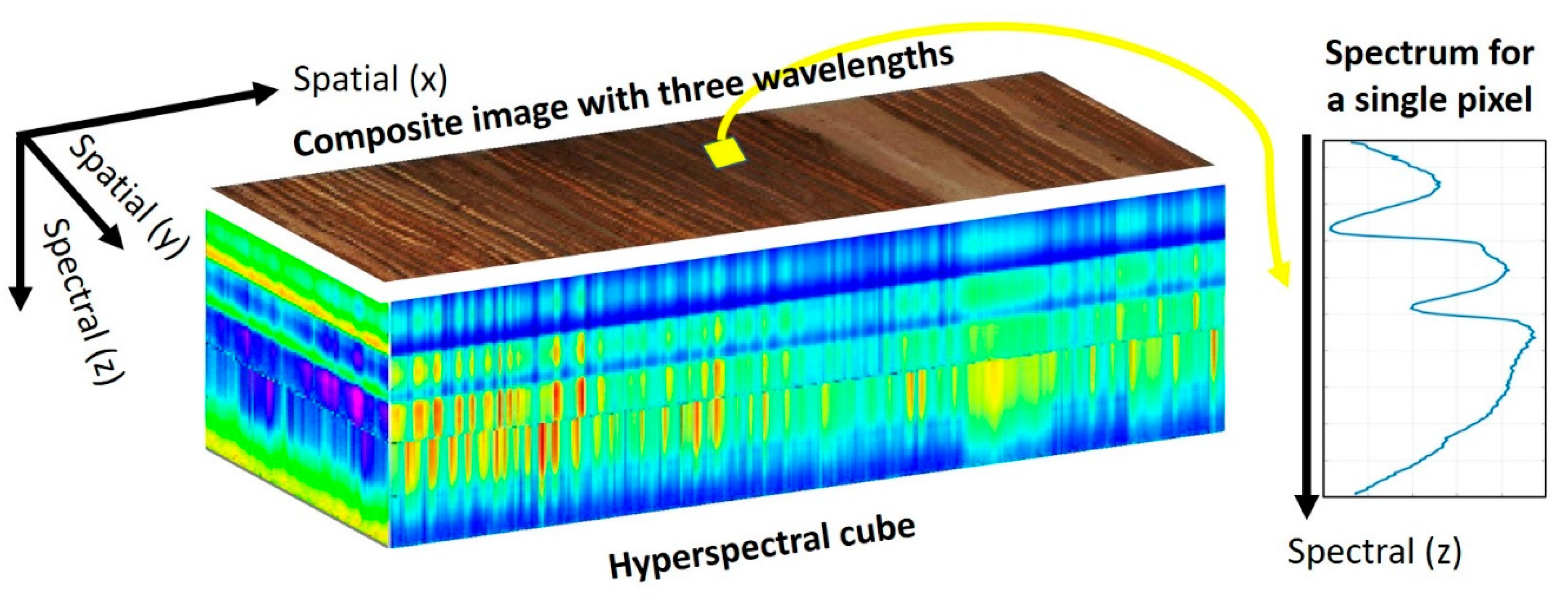
2. What Is Hyperspectral Imaging?

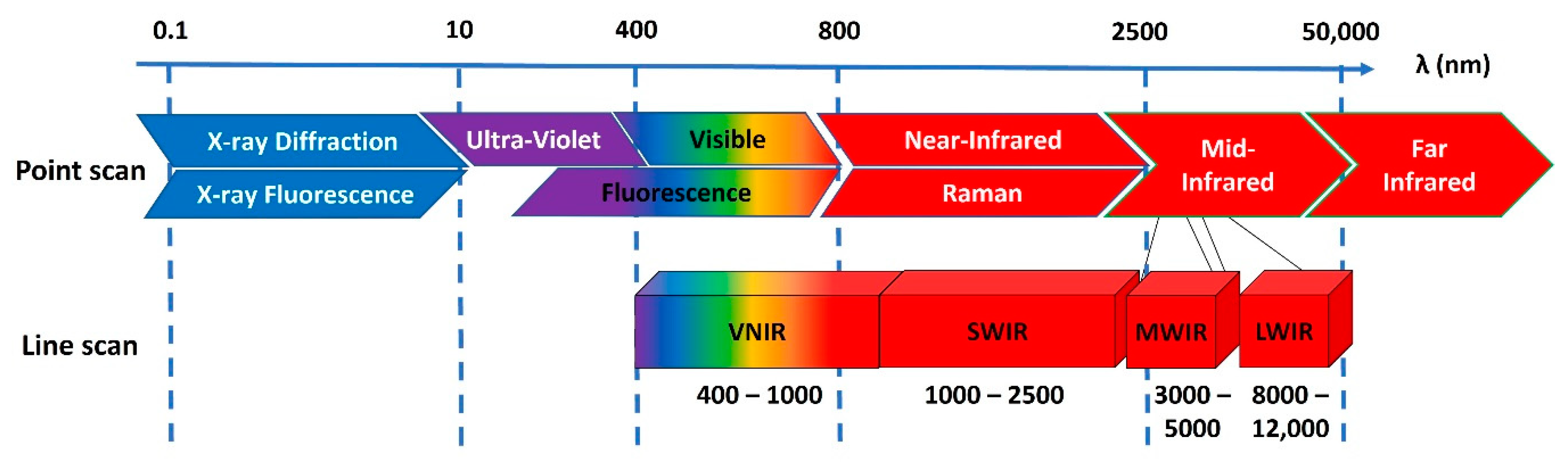
2.1. Hyperspectral Sensors

There are three ways to perform hyperspectral image acquisition. The first is the “whiskbroom scan”, which collects the spectrum one pixel at a time and has the highest spatial and spectral resolution but also the lowest speed. Then, there is a linear scan called “push-broom scanning”, which has a higher speed but a lower spectral resolution and suffers from a one-dimensional spatial limitation due to the detector (only a fixed number of pixels per line). The last is planar scanning, which has a high scanning speed but a low spectral resolution and suffers from a two-dimensional spatial limitation (only fixed numbers of pixels per row and column).

With high spatial resolution on the order of hundreds or fewer micrometers, high spectral resolution with hundreds or thousands of available wavelengths, and a consistent scan rate of minutes to hours point and line scanning are the most appropriate methods for the analysis of natural archives. Thus, the HSI can be obtained over most spectral ranges (Figure 2).

In the following, we will focus on push-broom sensors, frequently called core loggers, that are used on analysis benches to cover the ranges between the visible and mid-infrared wavelengths (Figure 2). Four main types of hyperspectral cameras from different manufacturers are available on the hyperspectral core-logging market. The visible and near-infrared (VNIR) camera covers the range of 400–1000 nm, allowing the detection of photosynthetic pigments (chlorophylls) and bacterial pigments (bacteriochlorophylls) [52,53,54,55,56], iron oxides, and altered organic matter [57]. The short wave-infrared (SWIR) sensor, which acquires a spectrum between 1000–1700 nm or 1000–2500 nm, allows the study of organic compounds (aromatic, aliphatic) [58,59,60] and types of deposits (clays, carbonates) [61,62]. The mid-wave-infrared camera (MWIR) operating between 3000 nm and 5000 nm allows the study of organic and mineral properties. Finally, the long wave infrared (LWIR), also called a thermal infrared (TIR), camera operating between 8000 nm and 12,000 nm allows the characterization of minerals [63,64]. The choice between these different sensors is made according to the study focus, as they provide different and complementary information, according to the constraints of these spectral domains and their characteristics (cost, speed, spatial and spectral resolution).

2.2. Acquisitions and Recommendations

Two main protocols have been published for HSI acquisition of sediment cores and they can be used for any other natural sample. The protocol of Butz et al. [48] presents the main steps to obtain an HSI. Jacq et al. [65] advanced from the first protocol and took a step further to thoroughly describe the different acquisition parameters and their influence on the image.

These two protocols help define the conditions necessary for the analysis of a sample. It must be as flat as possible to be within the depth of field of the camera (to have a sharp focus in an image) and not create microstructures and illumination differences due to the roughness of the surface [66]. The positioning of the sample must be parallel to the camera. The depth of field is related to focal length, distance to the sample and pixel size. The latter is often minimized to obtain a precise measurement, which also leads to a limited depth of field, on the order of a few millimeters. This shows the importance of having the sample as flat as possible and well positioned to the camera. The sample must also have all the sediment structures visible to the naked eye, if possible, so it is necessary to clean its surface. To prevent specular reflection caused by moisture on the surface of the sample, it should be left at room temperature for a few minutes to stabilize its moisture content.

The different acquisition parameters, discussed below, must be optimized according to the study issues.

In the case of a manual focus, it must be adjusted as finely as possible to obtain a sharp image (Figure 5a). This step is usually performed on a test pattern or an object with light and dark alternations. In cases of poor focus, we will observe a grayish image that represents a mixture of images containing two types of bands, and an optimal focus will end up distinguishing the two-color levels.

The integration time is the time during which the light will be collected by the detector. The longer the time is, the greater the signal-to-noise ratio. However, if the integration time is too long, this can cause signal saturation because the detector can only receive a limited number of photons. It should be based on the areas that are most reflective, usually the bright areas of the sample or white reflectance (Figure 5b). The integration time should be set at 75% of the saturation time of the signal, so the signal-to-noise ratio will be optimal without saturation.

Then, it is necessary to define the frame rate (number of pixel lines acquired per second). Considering that the maximum acquisition time of a line corresponds to the integration time, it is suggested to use 75% of this value because the detector read-out time must be considered.

Finally, to obtain the actual shape of the sample (square pixel), as shown in Figure 5c, it is necessary to define the scanning speed, which corresponds to the size of the pixel width divided by the frame rate; the former depends on the field of view (FOV) and the number of pixels in a line. To confirm the correct speed setting, it is recommended to check the ratio between the lateral and longitudinal dimensions of a known object until it corresponds to reality.

Thus, these parameters are related and must be defined together to obtain a relevant image with sharp focus and true dimensions (Figure 5).

Once all acquisition parameters are set, a sample can be imaged in three steps. First a black reference is imaged to estimate the instrumental noise (Sblack), then a white reference is imaged to calibrate the signal in percent reflectance (Swhite), and finally the sample (Sraw) is imaged. Normalization is performed for each spectrum (Sraw) by removing the instrumental noise from the black reference (Sblack) and the reflectance is calibrated in percent reflectance based on the white reference (Swhite), as shown in Figure 6. Thus, to have a well-parameterized exposure time to avoid saturating the image, Swhite is needed to conduct relevant normalization. Regular quality control of the Sblack and Swhite images allows us to verify the correct operation of the hyperspectral bench components because if a new disturbance (noise, dirt, aging) appears, it may indicate a problem that must be corrected (illuminant, detector, etc.). There are several types of white references calibrated according to their percentage of reflectance; therefore, using a reference whose percentage is close to that of the sample will maximize the signal-to-noise ratio.

It is also necessary to consider the possible aberrations due to the shape of the lens. A square pixel is produced in the center of the image, but geometric distortions are induced away from this point. The image of a ruler allows us to verify that the space between the graduations is always the same. Figure 7a shows a reduction of this space further away from the center, with 1 mm corresponding to 19.5 pixels in the center (1 pixel = 51.28 µm), against 17.5 pixels on the edges (1 pixel = 57.14 µm), so there is a distortion of approximately 5.86 µm on the edges with our lens. A correction of this effect can be done by modeling the distortion and correcting it for all of the lines of the image. We can also observe shifts in the wavelengths of the pixels when we move away from the center (the smile effect) [67]. To observe this, it is necessary to image a uniform sample such as the white reference. Figure 7b shows shifts in the spectrum toward smaller wavelengths between the center and the edges. A model of these shifts allows us to correct these errors.

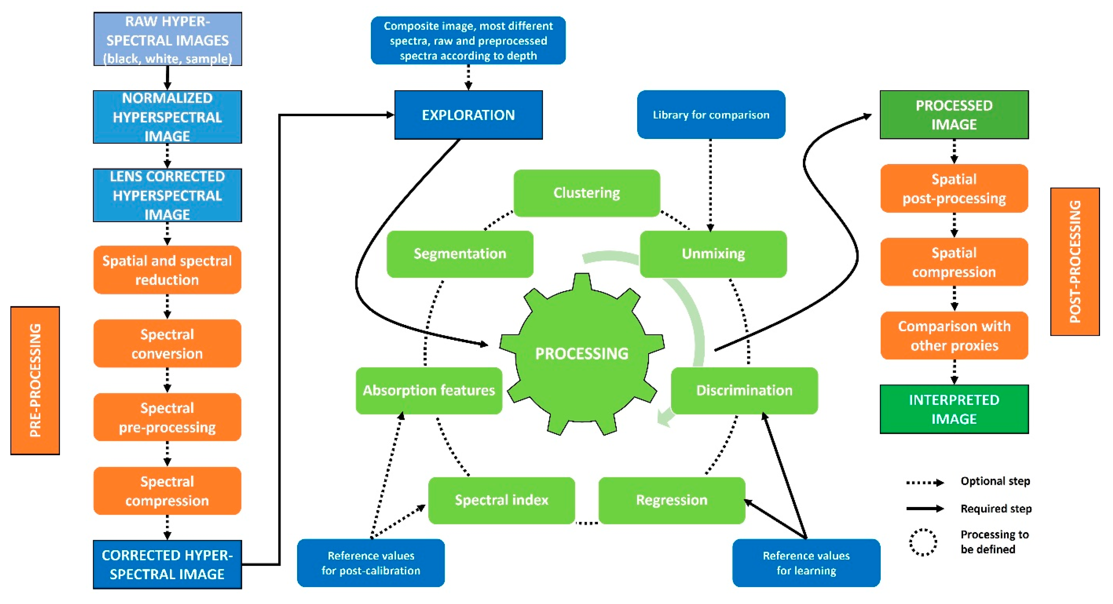
3. How to Process These Data?

To identify sedimentary processes recorded by hyperspectral data, four main steps are to be followed, fully or in part, as shown in Figure 8 [68]. (1) The first is to prepare the data by reducing the image to the spatial and spectral areas of the study and to use preprocessing to reduce the noise present in the data. (2) The second allows us to observe the first trends in the HSI, both in the spectral dimension with absorptions of some compounds and in the spatial dimensions with sedimentary deposits. (3) Data processing methods will allow us to extract these first observations and to highlight other properties of interest with machine learning approaches. (4) The maps extracted by these methods can be spatially postprocessed to reduce the residual noise or to match the observations with other analyses. This last step can help to confirm the observations and to obtain an interpretation of the biophysical-chemical properties recorded by the hyperspectral sensors. All the methods discussed below are not exhaustive, they simply aim to allow the reader to have some idea of the approaches found in the literature. MATLAB routines to perform some of these processing are available on Zenodo [69].

3.1. Preprocessing

An HSI may contain acquisition and sensor noise and contains a large amount of data that can be complex to process. It is therefore necessary to remove some spatial or spectral areas and use one or more preprocessing or compression steps [70]. Therefore, a sequence of four steps must be performed in whole or in part.

3.1.1. Spatial and Spectral Reduction

The first step is to reduce the HSI, in terms of both spatial and spectral dimensions, to have less data to process and thus accelerate the processing time.

A region of interest (ROI) can be selected to eliminate irrelevant areas such as surface variations due to certain holes and cracks or geometric aberrations due to the lens. The selection of an ROI also allows the keeping of a specific area representative of the whole sample to facilitate processing, which can then be applied to unselected data. This selection can be done manually on the data or semiautomatically on the object with the use of markers surrounding the study area that will be detected by software [71]. The mean reflectance image (Rmean) can also be used to create a mask indicating the exploitable pixels and the aberrant ones (low Rmean: holes, cracks; high Rmean: saturation), which will not be used in further processing.

Similarly, noisy wavelengths, often those at the ends of the sensor range, can be removed based on the standard deviation of the spectra or signal-to-noise ratios. Spectral areas of interest can be selected, and other interfering areas can be removed.

To reduce the data, the HSI can be under sampled with a binning that defines a sampling step to use for keeping a certain number of pixels and/or the number of wavelengths.

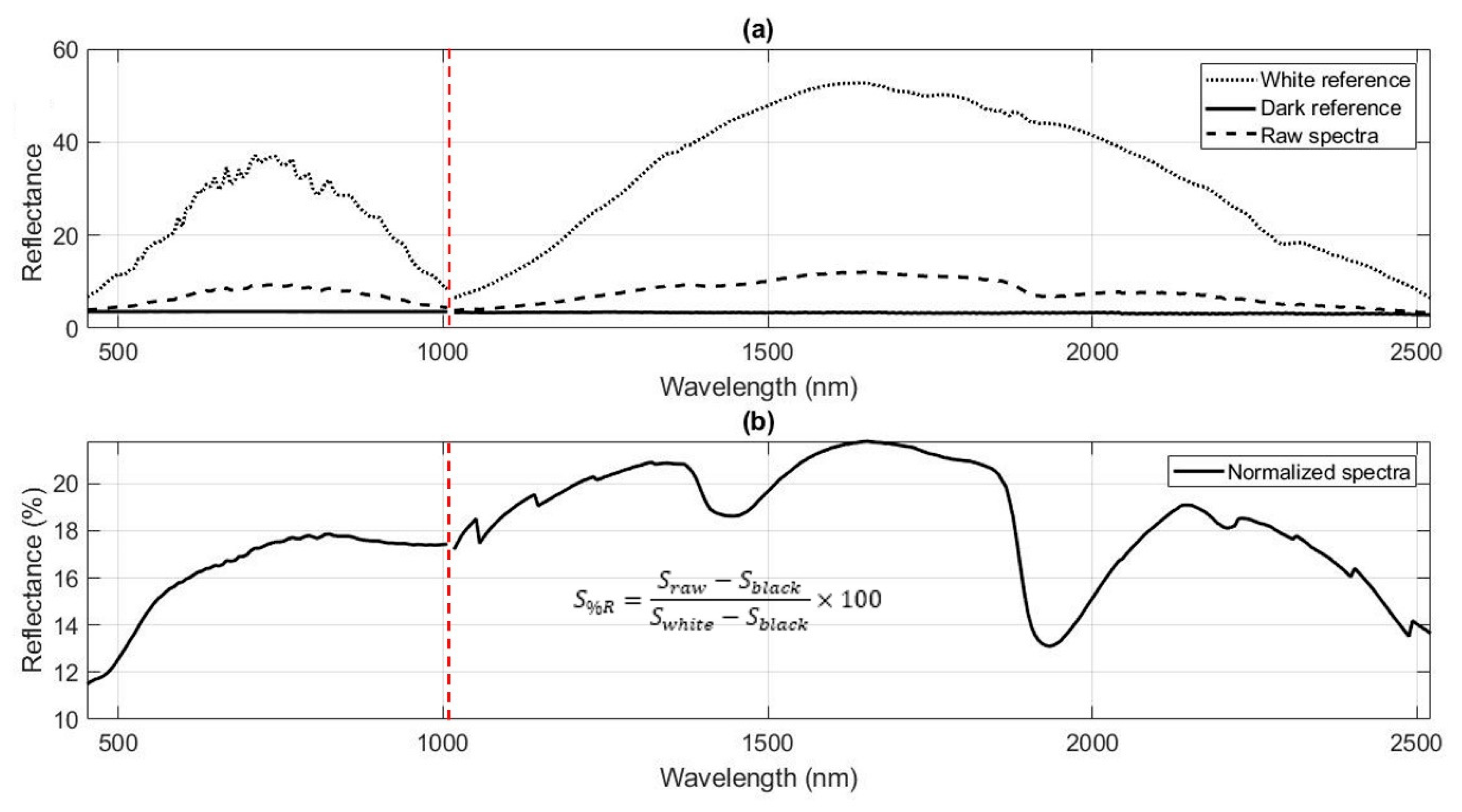
3.1.2. Spectral Conversion

The third step is useful for some of the processing approaches, which are presented later, and are based on linear models of the variables of interest. However, reflectance is not necessarily linearly related to the concentration of the compounds, so it may be important to convert the data into pseudo-absorbance.

According to Beer Lambert’s law [72], the concentration (c) of a chemical compound follows a linear relationship (within a certain range) as a function of the absorbance (A), molar attenuation coefficient (ε), and pathlength through the sample (l). It is therefore interesting to convert data between reflectance (R) and pseudo-absorbance (A) to find this linear relationship between absorbance and concentration of a compound of interest.

$$A=\epsilon \times l\times c\approx {\log }_{10}\frac{1}{R}$$

3.1.3. Spectral Preprocessing

The third step uses spectroscopic preprocessing to correct three main effects impacting the signal or to highlight spectral information [73,74].

The first effect is a noise term caused by stray light, the electronic noise of the detector. Several approaches to signal processing exist, such as moving averages or medians, polynomial smoothing, the use of Fourier transforms or wavelets. This term is classically reduced with smoothing in a moving window [75].

The second effect is a loss term due to the loss of photons between the emission by the illuminants and the reception by the detector. This effect affects the baseline; hence, the detrending method is classically used [76]. In remote sensing and for the spectroscopic characterization of rocks, the continuum removal method is used; it consists of modeling the shape of the spectrum with broken lines, but it requires a computing time that can be important [41]. The use of derivatives is also often adopted because it corrects this effect and can put forward information of interest [75].

The third effect is due to the dispersion of photons with the stretching of the optical path and photon penetration between the sediment grains. To correct it, two approaches can be used. The first is the logarithmic transformation, which also has the advantage of converting the reflectance data into pseudo-absorbance as we have seen previously. The second is to normalize the signal. Two preprocessing methods are classically used: the standard normal variate (SNV) [76] or the multiplicative scatter correction (MSC) [77], which normalize the signal with their mean and standard deviation or other parameters.

Finally, it is also possible to use these spectroscopic preprocessing steps in combination to correct several effects and to highlight spectral information. It should be noted that preprocessing influences the raw signal and can remove negative effects, but it can also create or remove information, so it is necessary to take a step back and control the effect. The choice of preprocessing is therefore made by always making a compromise between the observation of the data, the characterization of the effect impacting the spectra, and the performance of the models as carried out afterward.

3.1.4. Compression

Data compression also reduces the computation time and redundancy within the data. Principal component analysis (PCA) and minimum noise fraction (MNF) compress the spectral dimension into orthogonal components that contain the covariant spectral information [78,79]. In addition, choosing a low number of components also reduces the noise that is often contained when using a higher number of components. These approaches are therefore interesting to use to more easily visualize the spectral information that changes within the sample with a few variables rather than several hundred variables. However, this compression can also eliminate some small-scale information that is important for the study of some properties.

Compression can also be achieved by variable selection methods that allow us to keep only some of the wavelengths and to remove those that contain similar or information nonessential for the problem [80,81]. These approaches are generally used within supervised learning algorithms to estimate a link between wavelengths and a variable of interest. It can also be done by manually selecting the interesting channels based on absorption knowledge regarding the variable of interest.

3.2. Exploration

Before performing machine learning processing, it is recommended to visually examine the HSI and begin to identify its patterns to understand the sample and the data. To do this, there are several ways to visually examine HSIs based on spatial dimensions, spectral dimensions, or a combination of the two.

3.2.1. Composite Images

With the spatial dimensions, it is possible to estimate composite images from three channels of the HSI to characterize successive sedimentary deposits and thus make assumptions about the sedimentation processes. Table 2 shows the wavelengths of some classically used images.

Image processing also uses color space changes, such as HSV (Hue Saturation Value) or L*a*b* (Luminance, Chrominance), which have shown better segmentation capabilities than in RGB space [82,83,84]. These spatial changes can be applied to composite images extracted from the HSI.

The mean reflectance estimate can also be used as a grayscale image, so it can indicate dark or light pixels.

Table 2. Example of composite image estimated from HSI.

Sensor–Name	Name	Wavelength	Reference
VNIR	RGB (Red Green Blue)	640—545—460 nm	[48]
VNIR	CIR (Color InfraRed)	860—650—555 nm
VNIR	NIR (Near InfraRed)	900—800—700 nm
SWIR	pRGB (pseudo RGB)	2162—2199—2349 nm	[85]
SWIR	Hydrocarbon	1722—1760—2311 nm	[86]
SWIR	Hydrocarbon	1722—2311—2349 nm

Table 2. Example of composite image estimated from HSI.

Sensor–Name	Name	Wavelength	Reference
VNIR	RGB (Red Green Blue)	640—545—460 nm	[48]
VNIR	CIR (Color InfraRed)	860—650—555 nm
VNIR	NIR (Near InfraRed)	900—800—700 nm
SWIR	pRGB (pseudo RGB)	2162—2199—2349 nm	[85]
SWIR	Hydrocarbon	1722—1760—2311 nm	[86]
SWIR	Hydrocarbon	1722—2311—2349 nm

3.2.2. Spectral Visualization

The spectral dimension allows characterizing the physical, chemical, and biological variations within the sample. To represent them, the mean and standard deviation spectra allow us to see the dominant variations in the sample. Local variations can be highlighted by extracting the most different spectra within the HSI, which can be done with the Kennard and Stone algorithm [87].

To highlight the absorptions, preprocessing methods, such as first derivative (FDS) or continuum correction, are commonly used [41,75]. The interpretation of the absorption zones is possible using a table created for certain properties [26,28,32,41,42,43,88,89].

To combine spatial and spectral dimensions, the spectra can also be related to depth to observe representative variations in some deposits. These representations allow us to see the dominant variations in the data, and the fine variations will be characterized with machine learning approaches.

3.2.3. Spatial and/or Spectral Distribution

Visualizing the whole hyperspectral cube is complex, but using straightforward tools such as histograms, Rmean or other properties, allows us to have a view on the distribution of values at one or all wavelengths. Thus, these distributions can highlight patterns within the sample that can be discriminated and spatialized with the definition of a threshold for one or more of the chosen parameters.

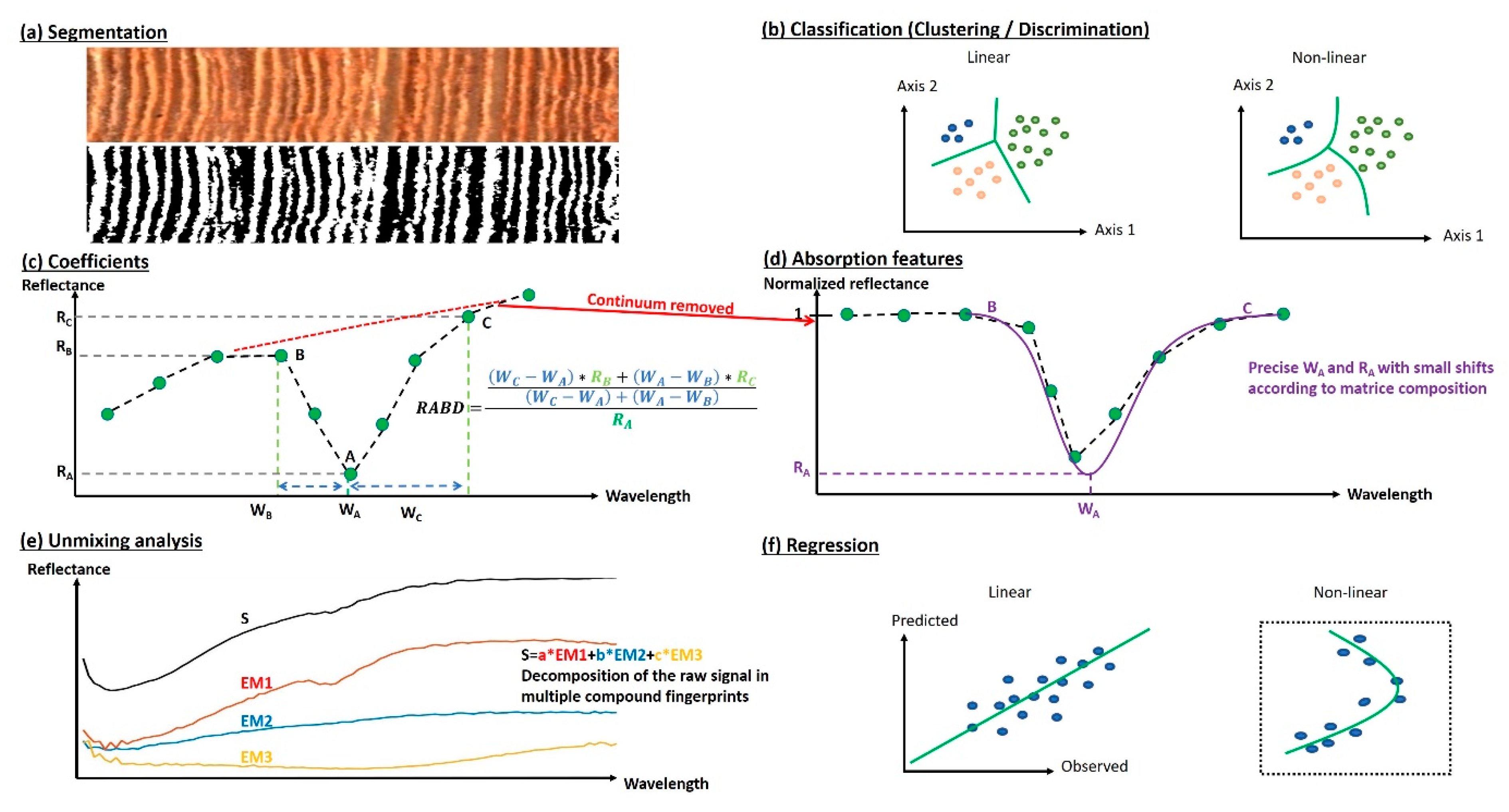
3.3. Processing

Various techniques exist for processing this type of data, and they can be divided into two groups depending on the dimension studied. Image processing focuses on the spatial dimension, while chemometrics, machine learning, and data mining focus preferentially on the spectral dimension but can also address the spatial dimension (Figure 9). The processing of HSIs must take into account these two dimensions to improve the knowledge of the sample. This is called the spatial/spectral duality [51]. All these approaches can also be divided into two qualitative and quantitative groups.

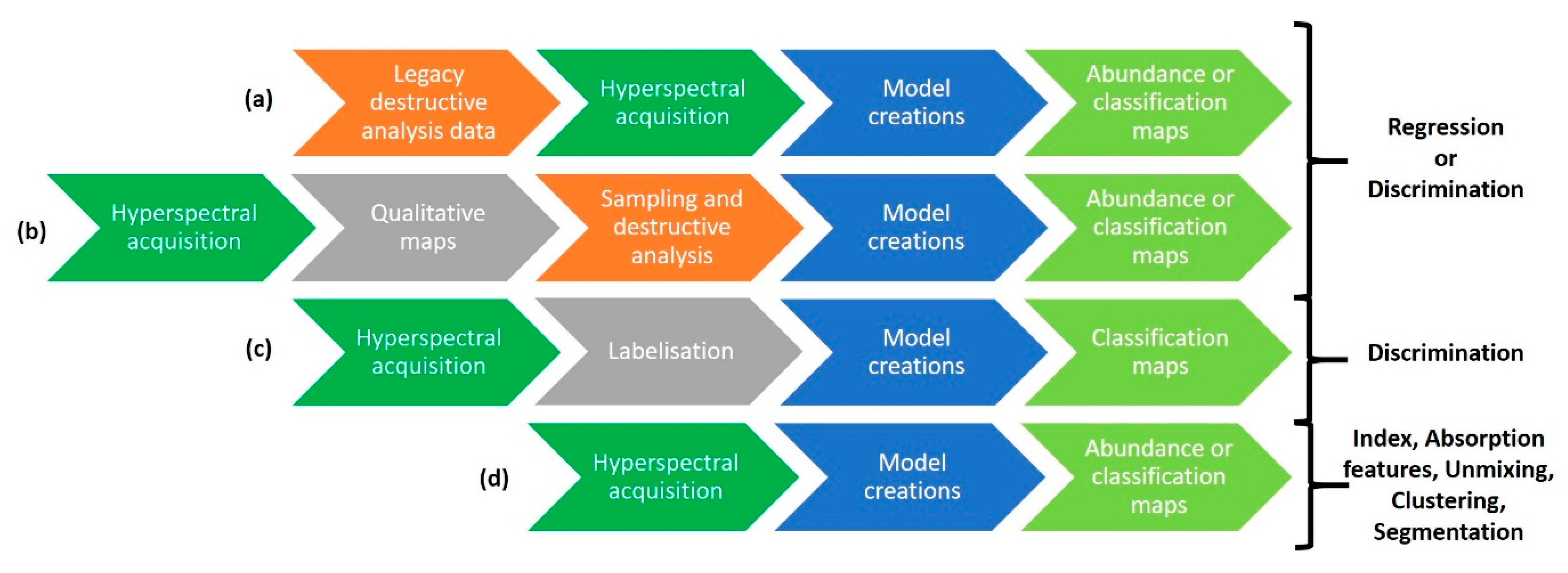
3.3.1. Qualitative Approaches

Qualitative approaches include (1) image segmentation and (2) classification methods.

(1) Segmentation methods are used to identify breaks in the continuity between neighboring pixels to divide them into several areas, or conversely, group regions with similar properties [11,90,91]. They allow the characterization of sample structures (strata, grains) by considering the relationships between neighboring pixels (Figure 9a). These methods are generally used on a grayscale level image and not on multiple channels such as an HSI, so a compression or wavelength selection step is necessary.

(2) Classification methods are divided into two groups, depending on whether the sample is known (labeled data, Figure 9b). (2a) In the case of unknown data, we refer to clustering; these methods will search for spectral similarities and divide them when they are dissimilar based on distance or variance criteria [92,93]. However, classical methods of this type may not be robust enough due to the high interpixel redundancy in the HSI [94,95]. This is why new approaches using neural networks or fuzzy logic are gaining interest [96]. (2b) In the case of labeled data, we refer to discrimination; these methods will estimate the relationships between the different known groups and maximize the distance or variance criteria between them to separate them [97,98,99,100,101]. Generally, these classification methods do not use the relationship between neighboring pixels but only spectral data. For clustering, spatio-spectral approaches are emerging based on deep neural networks [102,103,104]. Many classification methods exist, and there is not a universal one, which is why it is necessary to test several methods based on different hypotheses and to determine which one will be best able to answer the problem [105]. It should also be noted that these methods will be specific to the data they have learned, so a model developed on a core from one site may not apply to a core from another site that may have different sediment variability and therefore different spectral variability.

3.3.2. Quantitative Approaches

Quantitative approaches can be divided into four groups: (1) indices, (2) characteristic absorptions, (3) pure signals, and (4) regressions. As far as the classification method is concerned, these quantitative approaches are specific to the data they have learned for each intended site and therefore will not be usable on another site with different sedimentary and spectral variability.

(1) The study of specific sample properties has made it possible to identify characteristic wavelengths that are used to create indices that allow the estimation of a semiquantitative value (Figure 9c). Many indices have been developed for the study of chlorophyll pigments or to characterize some minerals, such as iron oxides, clays, and calcites [26,48,106,107,108]. These are based on reflectance differences, ratios at defined wavelengths or the estimation of the area or height of the absorption peak in the spectra, as shown in Van Exem et al. [50] for the chlorophyll pigment indices. The use of these indices relies on the prior investigation of the spectra and the visualization of absorptions in these characteristic zones. It is also necessary to consider the possible overlaps between several chemical compounds that can absorb in the same wavelength range. These indices provide a semiquantitative estimate of a property, and it can be interesting to calibrate them with specific analyses of the investigated property. If sampling is necessary, its scope can be defined using these semiquantitative values to limit the number of samples.

(2) For some properties, it is also informative to consider the wavelength shifts in some spectral regions where several compounds may be present [109,110] (Figure 9d). In particular, the area near 2.200 nm is characteristic of clays with the absorption of Al-OH bonds such as illites that absorb at 2.205 nm, smectite at 2.205 nm and 2.230 nm, kaolinite at 2.160 nm and 2.208 nm [31]; or near 2.350 nm with micas at 2.350 nm, chlorites at 2.325 nm and 2.360 nm, calcite at 2.340 nm, and illites at 2.350 nm [88]. It is therefore complicated to focus on a few wavelengths without prior knowledge of the sample due to the numerous overlaps between several properties, and care must be taken when interpreting the abundance maps obtained with these first two methods. This approach consists of the correction of the signal from its continuum and then modeling the different absorptions with a Gaussian function [109]. These steps are computationally time-consuming with multiple modeling and peak characterizations. Similar to the indices, these estimates can be confirmed and calibrated with additional sampling and analysis.

(3) The overlapping of absorbing compounds in the spectral areas can be estimated with some approaches amed at the characterization of pure signatures, called endmembers (EMs). Indeed, a spectrum is a sum of signals corresponding to all of the compounds present in the sample (Figure 9e); thus, it is possible to dissociate these signals to find pure signals that are then characterized by comparing them to libraries or with other analytical methods [111,112]. An EM can be a pure compound such as a mineral (clay, chlorite, etc.) or a sum of compounds representing a source in the watershed. These approaches allow us to perform what is called a subpixel since a pixel will be characterized by several pure sources, so it will be possible to have a repartition of each source within a pixel. The user must generally define several EMs that are difficult to find without prior knowledge of the number of sources that can be characterized by the sensor. Comparison of EMs with spectral libraries is questionable because these spectra are not representative of what is detected with a specific sensor in the laboratory. Among the available libraries, we mention those of the United States Geological Survey (USGS) [113], Commonwealth Scientific and Industrial Research Organization (CSIRO) [114], and ECOsytem Spaceborne Thermal Radiometer Experiment on Space Station (ECOSTRESS) [115]. For this reason, it is advisable to create a library of compounds from the sensor used; these sensor-specific spectra are then used to unmix the hyperspectral signal. This is called the sparse unmixing method [116,117,118].

(4) With regression approaches, these known data are directly related to the spectra [119,120,121,122,123] (Figure 9f). The developed regression model estimates specific coefficients for each wavelength; the larger this coefficient is, the more important this wavelength is for predicting the studied property. These can correspond to specific wavelengths of the property or correlated information. In contrast, wavelengths with low coefficients carry little information related to the studied property, and it is recommended to remove them because they can harm the predictions. As with classification methods, there are many regression methods, and several must be tested to estimate which ones best fit the problem.

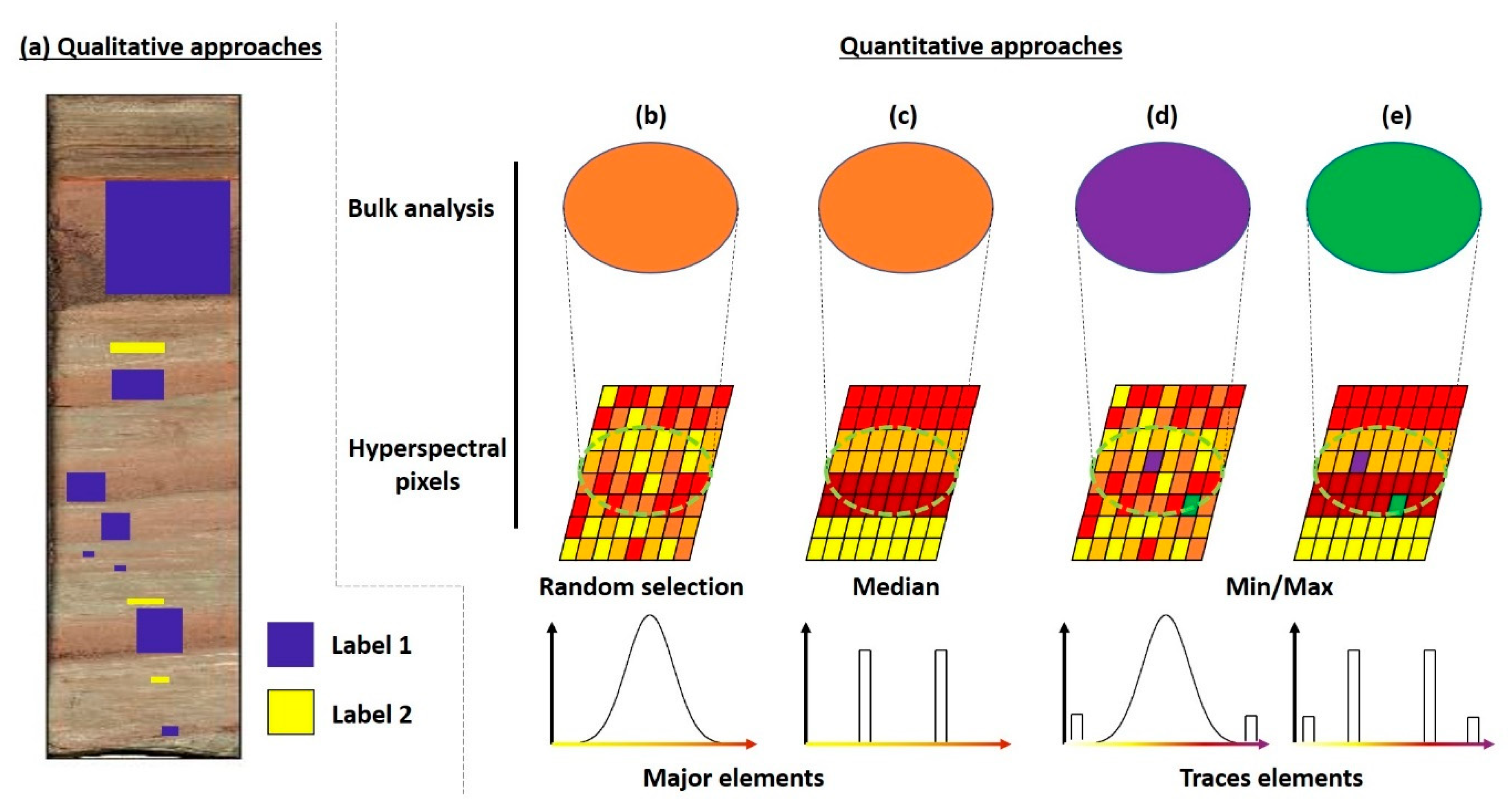
3.3.3. Subsampling for Model Calibration (cm vs. µm)

The development of a predictive model requires a spectrum to provide reference data (label or quantitative value). It is therefore necessary to select regions of interest (ROIs) corresponding to the reference values. Two strategies can be used depending on whether the data are qualitative (label) or quantitative.

Qualitatively labeled data are usually related to manually or automatically labeled pixels (Figure 10a). All these pixels are then used to calibrate and validate the prediction model.

For quantitative references, the destructive sampling position is usually known within a specific range, so it is necessary to select the corresponding pixels. Creating a predictive model requires subsampling a spectrum to obtain a reference value [49]. proposes several approaches depending on the distribution of the reference to be characterized. The simplest case for global references with a discrete distribution, which can also be used in the case of an unknown distribution, is to use the mean or the median value of the spectra corresponding to a reference (Figure 10c), but this may remove the minority information in the signal. Therefore, in the case of a global variable with a Gaussian distribution, it is recommended to perform successive random selections to estimate a set of optimal and most representative spectra of the reference studied to preserve the minority variations (Figure 10b). Finally, in the case of a trace reference, other subsampling statistics are to be used, such as the minima and maxima (Figure 10d,e).

Quantitative models are created using destructive analyses that are usually performed following a continuous or visual sampling design before hyperspectral analysis (Figure 11a). This does not necessarily correspond to the most representative concentration ranges or spectral variabilities of the sample. Many specific indices and wavelengths can be used to create semiquantitative abundance maps of some properties. Thus, their studies can indicate the areas to sample to cover the maximum variability of the sample and to limit the number of samples (Figure 11b). They can also be useful for image labeling for discrimination approaches, which also require incorporating a large amount of spectral variability to be more robust (Figure 11c).

A destructive analysis generally corresponds to an average value of the sampled area; with the higher resolution of the HSI, it is, therefore, possible to predict values outside the calibration range. These values will therefore be questionable since the relationship outside the calibrated range may be nonlinear. To obtain a relevant range, it is necessary to sample at a resolution close to that of the HSI, which is rarely possible, or to sample in homogeneous areas with a relevant sample resolution. Similarly, visual labeling is user-dependent, which can lead to poorly labeled pixels that will induce a bias during the learning phase. Only an “analytical ground truth” at similar resolutions will be able to confirm the relevance of the prediction models, which can be done for the study of minerals by microscopy, but not at the moment for other variables.

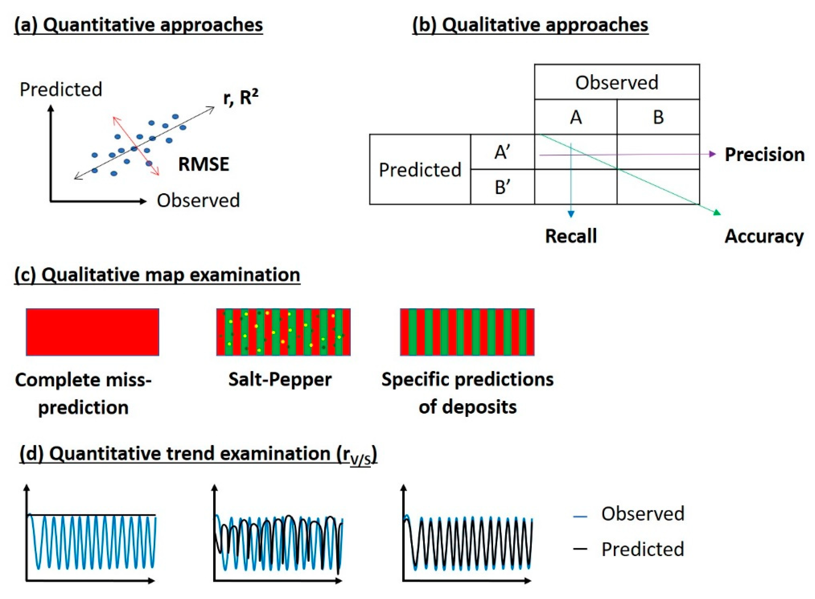
3.3.4. Model Validation and Performance

For methods calibrated with reference values (qualitative or quantitative), it is necessary to validate the models prior to estimating their performance. For regression methods, quantitative validations are generally performed using correlation or determination coefficients and root mean square errors allowing the calculation of the prediction uncertainties, as presented in Figure 12a [125]. For discriminant methods, model performance is estimated using classification indicators (accuracy, precision, recall, F-measure), as represented in Figure 12b. For both methods, a qualitative examination of the predicted map (Figure 12c) is also performed to check the quality of the prediction (no salt and pepper character, continuity of the prediction in a structure). A correlation between the reference data and the trend of the subsampled prediction (median value of the map) must be estimated, and it is noted as r_V/S [60] (Figure 12d).

Some modeling methods also identify discriminating wavelengths that can be associated with physicochemical properties to interpret the model and verify its validity. The classification or regression map can also be used to verify the model based on the environmental knowledge of the sample, and some areas may be associated with a specific class or specific values compared to another.

3.4. Post-Processing

Once the hyperspectral data are processed, specific maps of properties of interest are obtained. In some cases, the relevance of the prediction can be increased by studying the neighboring pixels with spatial postprocessing. Two strategies can be used to reduce some spatial artifacts (specular reflection, hole, crack, salt and pepper effect). The first consists of using image filters to average neighboring pixels to smooth the map or by applying contrast enhancement to improve the separation between deposits [126]. The second is to compress the image to reduce local effects or to match the image resolution with that of other data. These two approaches are based on windows that can have different shapes (square, circle) and functions (average, median, mode) [126,127]. These methodologies smooth the map, reduce the salt-and-pepper effect and outliers but can remove nugget effects and cause false structures to appear. Therefore, for the preprocessing stage, it is necessary to choose the postprocessing carefully and check the impact it has on the image.

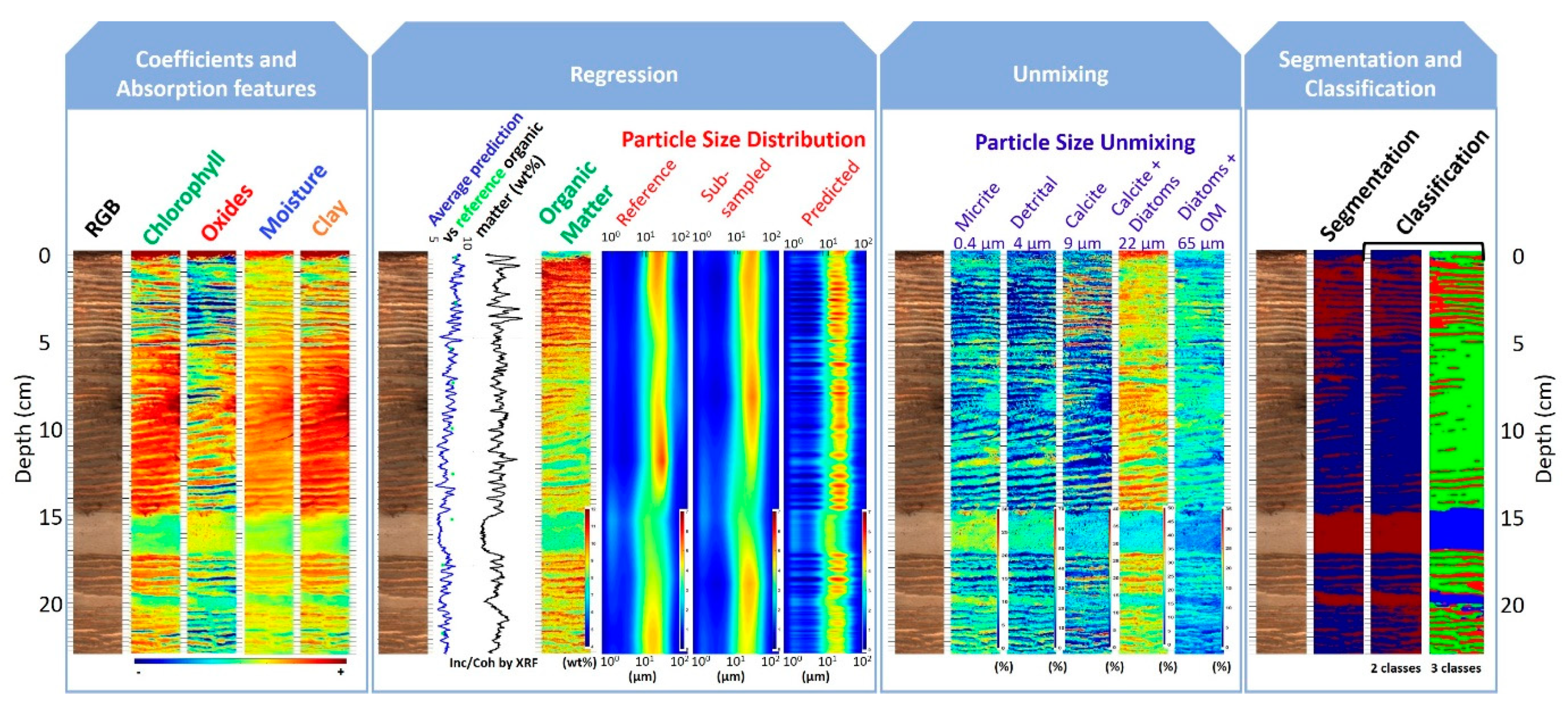
4. What Sedimentary Properties Can Be Derived from It?

In addition to the few cases of sediment core analysis, we also review researches from related fields, such as sedimentary rocks, soils, and remote sensing. Below we present five major themes that aim to reveal the various sedimentary properties with the use of HSI and versatile methods. (1) The trophic status of lakes is extensively studied by spectroscopy, and HSI can take advantage of this work by leveraging specific pigment indices. (2) Source-to-sink studies can also be performed using spectral fingerprints (endmembers EMs) associated with sources in the lake catchment. (3) Organic matter is an important sediment property for paleoenvironmental reconstructions or the estimation of anthropogenic pollution and is generally characterized with regression/classification approaches or index definitions. (4) Sediment mineralogy is also an important property used to describe the sources of sediment supply within the watershed, and it can be characterized with indices or regression and classification methods. (5) Sedimentary structures and texture will have spectral and/or spatial fingerprints that can be recorded by HSI and characterized with classification methods. Figure 13 shows groups of the different approaches according to the topic and allows the visualization of the links between Section 3.3 and the following paragraphs. Another recent hyperspectral imaging review by Zander et al. focuses on the biogeochemical analysis of sediment cores and is complementary to the review above [128].

4.1. Trophic Status

The trophic status of lakes and water bodies is mainly estimated according to the microalgae and bacteria once present in the water column, which are subsequently trapped in the sediments. Some of them can be characterized by pigments, such as chlorophylls and their derivatives, carotenoids, bacteriochlorophylls, etc. Some compounds, such as chlorophylls, have been studied for a long time by visible spectroscopy, which has led to the creation of many indices (Table 3) that can be applied to HSI. Currently, two spectral areas are widely used with the VNIR camera data. The first is specific to chlorophyll a (Chl a), pheophytin a (Phe a) and their derivatives, which can be identified by integrating the absorption area of these compounds in the range from 584 nm to 730 nm (Area584-730) or measuring their absorption peak height [52,53,54,55,56]. Chl a allows the reconstruction of aquatic productivity within the lake. The second index focuses on bacteriochlorophyll a (BChl a), bacteriopheophytin a (Bphe a) and their derivatives with the integration of the area between 790 nm and 900 nm (Area790–900) or the height (RABD845) [48,52,55,56]. Bphe a is a bacterial pigment product produced by the degradation of bacteriochlorophyll a (Bchl a) at the chemocline of meromictic lakes by anoxygenic phototrophic bacteria. Using sedimentary Bphe a allowed us to infer episodes of meromixis (i.e., long-term hypolimnetic anoxia) and mixing conditions by seasonal changes of temperature or event-based water mixing [48]. Another index to characterize the trophic status of lakes and their oxygenation has been proposed by Yacobi et al. [129] that uses phycocyanin. Indeed, phycocyanin is typically found in mesotrophic and eutrophic inland waters dominated by cyanobacteria. It was used by Sorrel et al. [56] with a RABA600—630 index that integrates the absorption area between 600 nm and 630 nm specific to this compound, overlapping with that of chlorophyll a. As no correlation existed with RABA630—700, the hypothesis of the predominance of phycocyanin was retained. Next, these semiquantitative estimates are calibrated with data from high-performance liquid chromatography (HPLC).

Many indices exist in the literature to study Chl a and its derivatives, as mentioned by Van Exem [50]. The author notes that most are site-specific and others require corrections based on the surface condition of the sediment core. If the core is rich in iron oxides, he shows that dividing the indices by the first derivative at 555 nm (d555) [22] allows us to improve the predictions. Similarly, if the samples are oxidized by ambient oxygen or have refractory organic matter (OM), he recommends dividing the indices by the mean reflectance of each spectrum (Rmean). However, as the variability within a sample can be important, it is possible to find different areas corresponding to these two properties, so it is necessary to develop an automatic step to determine whether to normalize, or not, and if so, by what.

Other pigments have also been studied by spectroscopy in the visible range but are difficult to estimate because they overlap with other compounds. Carotenoids absorb near 510 nm, which corresponds to a region where the oxides absorb a lot and mask their presence [130]. Other pigments have also been characterized in solvents by visible spectroscopy, such as chlorophylls b, c, d, and f, or bacteriochlorophylls b, c d, e, and g, but the sedimentary matrix can mask them [28,131,132]. That being said, the use of multivariate regression approaches may allow the separation of overlapping compounds and even the identification of minority compounds. Some organic pigments, such as chlorophylls, bacteriochlorophylls, phycocyanins, and phycoerythrin, also have chromophoric parts that make them fluorescent and therefore detectable with adequate excitation light [131,133,134,135].

Table 3. Some spectroscopic pigment coefficients for the ultraviolet, visible, and near-infrared spectral ranges reported in the literature for different samples (sediments, rock, soil and water).

Variable Studied	Coefficients	Wavelengths Used (nm)	Reference
Chlorophyll a + derivatives	d675	675	[136]
Chlorophyll a + derivatives	Area650—700	650–700	[27]
Chlorophyll a + pheophytin a	RABD590—730	590, 690, 730	[53]
Bacteriopheophytin a	RABD845	790, 845, 900	[48]
Phycocyanin	aPC	625	[129]
Carotenoid	RABD510	490, 510, 530	[106]
Total pigment content	RABA400—560	400–560	[106]
Main sediment components	Q7/4	400, 700	[26]

Table 3. Some spectroscopic pigment coefficients for the ultraviolet, visible, and near-infrared spectral ranges reported in the literature for different samples (sediments, rock, soil and water).

Variable Studied	Coefficients	Wavelengths Used (nm)	Reference
Chlorophyll a + derivatives	d675	675	[136]
Chlorophyll a + derivatives	Area650—700	650–700	[27]
Chlorophyll a + pheophytin a	RABD590—730	590, 690, 730	[53]
Bacteriopheophytin a	RABD845	790, 845, 900	[48]
Phycocyanin	aPC	625	[129]
Carotenoid	RABD510	490, 510, 530	[106]
Total pigment content	RABA400—560	400–560	[106]
Main sediment components	Q7/4	400, 700	[26]

4.2. Source to Sink—Fingerprinting

The sediment is a combination of particles possibly coming from different sources in the watershed and those produced in the lake, while the spectroscopic signal is composed of the sum of signals that may correspond to these sources. Unmixing or clustering methods allow us to find “pure” numerical poles that can then be associated with sediment properties.

Van Exem et al. [57] used the VNIR spectrum to search for pure signals (endmembers) with the pixel purity index (PPI) method [137] in a sediment core from Lake Linné in Svalbard. They compared them to signatures of samples taken in the watershed, which allowed them to estimate the provenance of the sediment inputs. One of these signatures is correlated at 0.86 with the total organic carbon (TOC), thus allowing them to reconstruct these variations, which come mainly from a single source.

These unmixing approaches are most often used in remote sensing [138,139] or in sedimentary rock cores [140,141,142] where there are very different and distinct pure poles. With sediment cores, this is more complex because the sediments from different sources are usually mixed and therefore indistinct. Sellier et al. [143] showed that the mineralogical contributions of the distinctive sources are very different and therefore can be characterized, as shown by spectroscopic approaches in the visible [143,144], visible and near-infrared [145], or mid-infrared [146,147,148] regions, but these signatures must be identified first within the watershed samples. This work used data from mixtures of products from the watershed as the training material and training methods (discrimination or regression) to estimate the proportions of each source in a single sediment sample. Evrard et al. [147] showed that conventional geochemical methods exhibited similar predictions to the results from a regression model using mid-infrared data.

4.3. Organic Matter

Organic matter (OM) is an important sediment property to reconstruct the past environmental and climatic variations or to detect organic pollution. It is studied by different spectroscopic methods depending on the OM characteristics. The infrared ranges (near- and mid-infrared) are widely used because they record many organic bonds that allow characterization of the total OM, or specific (aromatic, aliphatic) compounds [32]. The visible range is used to trace pigmented OM mainly from algae and bacteria, as previously described.

The SWIR sensor was used to reconstruct the loss on ignition at 550 (LOI550) value, which is related to OM, with partial least squares regression for several sediment cores from different sites [49,60]. The work of Jacq et al. [60] also showed that these predictions correlate with other OM proxies, such as incoherent coherent ratios from X-ray fluorescence (XRF). It may therefore be possible to predict OM nondestructively at low resolution with XRF indicators such as the incoherent coherence ratio or bromine [33] and then estimate OM at high resolution by SWIR. However, care must be taken with these XRF and LOI550 indicators, which may incorporate properties other than OM [149,150]. This is why the author could not create a model integrating different sites since LOI550 did not track the same properties among the different sites. The variable to be predicted must therefore be sufficiently specific to be robust, such as with TOC by RockEval pyrolyzis or specific organic molecules. Moreover, these different models are specific to the studied sites through the sedimentary matrix effects that they have learned in addition to the variable of interest, explaining difficulties to transfer a model to another site unless they learn enough matrix variability to correct it.

Van Exem [50] with the VNIR sensor shows that the I-band [106], generally used to trace chlorophyll a and its derivatives, allows us to trace altered OM. They show that this index correlates at 0.73 with charcoal concentration. Moreover, the spectral first derivative signature is characteristic of altered OM [26]. As mentioned in the previous section, this sensor has also allowed us to trace this type of OM with spectral unmixing approaches [57]. There are also approaches discussed previously using indices to quantify organic pigments (chlorophylls, bacteriochlorophylls, etc.) [48,52,55,56].

Different types of OM in sediments and soils have also been extensively studied using spectroscopy due to their absorption in different spectral ranges. OM and organic carbon are the most commonly studied in the infrared range [31,151,152,153]. Organic carbon fractions, such as refractory carbon, hydrolysable carbon, and microbiological biomass, can also be characterized in these same spectral ranges with greater performance in the mid-infrared range [154,155]. Humic and fulvic substances are characterized by infrared and UV–visible fluorescence [156,157,158,159]. Hydrocarbons are analyzed in the visible and infrared domains, allowing paleoenvironmental studies or pollution detection. Several classes of hydrocarbons are defined as total hydrocarbons (TH), total petroleum hydrocarbons (TPH) or polycyclic aromatic hydrocarbons (PAH), and the latter two are also characterized by UV–visible fluorescence [160,161,162]. Finally, other organic pollutants, such as polychlorinated biphenyls (PCBs) [163], pesticides [164,165], and microplastics [166,167,168] are being analyzed by spectroscopy. These studies can potentially be performed with hyperspectral sensors on sedimentary samples, which shows that the current work of HSI is still in its beginning stages.

4.4. Mineralogy

Like pigments, many minerals absorb in the visible and infrared ranges. However, to our knowledge, only two studies have been performed that are specific to mineral characterization by HSI for sedimentary cores, so we will discuss this issue in the context of the related fields in the following material.

The first study on the mineralogy of the sedimentary cores is derived from grain size modeling. Jacq, et al. [169] used the combination of two VNIR-SWIR sensors to reconstruct the particle size distribution (PSD) of a core from the Lac du Bourget (France) with a multivariate regression method (partial least squares regression, PLSR). The deconvolution of the PSD prediction with Gaussian distributions allowed them to determine four sources of specific sedimentary grain size input signatures [170]. They were associated with micrite particles, detrital particles, small calcite crystals, larger calcite crystals associated with diatoms, and diatom frustules associated with organic matter. These sources were then associated with seasonality and this allowed the estimation of a sediment supply flux. This study also showed that there is a close link between the physical (particle size) and chemical (mineralogy, organic matter) properties.

The second study focuses on the characterization of three mineral classes (clay minerals, calcite, and quartz) [171]. They are characterized by Diffuse Reflectance Infrared Fourier Transform spectroscopy (DRIFTS) which is a fast and non-destructive method, but it is punctual and has a low resolution. Therefore, the authors use SWIR hyperspectral imaging and PLSR to estimate them continuously at a high resolution. The proposed models exhibit validation determination coefficients of 0.85 for clays, 0.64 for calcite and 0.70 for quartz. The authors notice that quartz is not active in the SWIR range, so the model uses wavelengths correlated to this property such as moisture and clays. They also noticed that the prediction of quartz is site-specific and may not be realized at other sites. The authors also suggest that DRIFTS analysis could be replaced by hyperspectral sensors in the mid-infrared range such as MWIR or LWIR.

Thus, many spectroscopic studies utilize references to specific wavelengths for some minerals that are quantified with indices, as shown in

Table 4. Some spectroscopic coefficients reported in the literature for the visible and near-infrared spectral ranges for different samples (sediments, rock and soil).

Variable Studied	Coefficients	Wavelengths Used (nm)	Reference
Oxides	d555	555	[22]
Goethite	d535	535
Hematite	d575	575
Lithogenic material (chlorite, illite, biotite)	R570/R630	570; 630	[106]
Lithogenic material (basaltic lithics)	R850/R900	850; 900	[173]
Clay content	BD2170—2270	2170; 2270	[108]
Clay content	SWIRFI	2133; 2209; 2225	[174]
Chlorite	IndexChlorites	2187; 2275	[107]
Kaolins	IndexKaolins	2153; 2192
Micas	IndexMicas	2139; 2200; 2294
Calcite	BD2340	2340	[175]

[88,172]. Krupnik and Khan [88] have identified the absorptions of silicates and nonsilicates (most of which absorb in the infrared range), except tectosilicates and phosphates (which are specific to the mid-infrared region), while colored minerals such as oxides also absorb in the visible region. They also highlighted the importance of selecting one sensor over another for individual mineral studies and discussed potential field prospecting for certain minerals, such as oxides, sulfides, clays, carbonates, rare earth elements, copper, and gold veins.

Therefore, several studies have identified absorption areas to estimate the wavelength shifts of absorbing minerals in nearby areas. Murphy et al. [176] used a VNIR camera in the region between 840 nm and 980 nm to differentiate hematite and goethite. The absorption area between 2180 nm and 2220 nm (SWIR) was used by Hecker et al. [177] to characterize the crystallinity of illite and muscovite, while Dalm et al. [178] used it to study white micas. In the same way between 2310 nm and 2360 nm, [179] studied a mixture of calcite and dolomite, while Dalm et al. [178] investigated chlorites. Thus, it is very useful to have initial knowledge of the sample mineralogy to estimate the areas that can absorb because in the most complex cases, several minerals and other soft sediment core materials can absorb in the same wavelength areas.

Sediment rock core studies use geochemical analyses coupled with supervised classification approaches to classify each pixel into a mineralogy type or estimate mixture components. Support vector machine (SVM) and random forest (RF) classification methods are the most commonly used—for example, coupled with VNIR-SWIR or SEM-MLA data to allow the differentiation of 14 mineral classes with 74% and 71% accuracy, respectively [61]. Schneider et al. [180] predicted six mineral classes using XRD with accuracies of 95.4% and 97.3% with the SVM and Gaussian process methods, respectively. The approaches of [63,64] go further by using several VNIR, SWIR, LWIR, and RGB sensors and combining their results with SEM-MLA to predict five classes of minerals with accuracies of 66% with 1 sensor versus 90% with the combination of all the sensors. These studies showed that while depending on a single sensor and its spectral range, a mineral may or may not be well predicted based on its response in that range. Nevertheless, these discrimination approaches may not reflect the reality where there may be several types of minerals in a single pixel, so it is necessary to quantify the part of each mineral within a pixel with regression approaches. Tusa et al. [61] used VNIR-SWIR sensors and RF, SVM, and artificial neural network (ANN) regression methods to predict the 10-class SEM-MLA levels with R² values of 0.83, 0.60, and 0.82, respectively, for one study sample. In the same way, Rivard et al. [62] used multiple linear regression (MLR), SWIR, and LWIR data to predict wavelength-dispersive X-ray spectroscopy (WDXRF) contents with R² values between 0.62 and 0.81.

A study of soils using a VNIR sensor and PLSR to predict the elements determined using inductively coupled plasma with optical emission spectrometry (ICP–OES) showed that the elements Cu, Zn, Mg, and Ca presented R² values between 0.73 and 0.81 and had total carbon and total nitrogen correlations between 0.75 and 0.90 [181]. This shows that we can trace a compound that has little or no absorption in a spectral range but is well modeled through correlation with other components.

Currently, many spectral areas of minerals are characterized and are used to qualitatively interpret hyperspectral data from sediment cores. Through studies of related fields, there are many opportunities for finer characterization of sedimentary mineralogical properties by HSI.

4.5. Classification and Identification of Sedimentary Deposits

Sediment cores often show deposits that are interesting to identify and characterize. HSI allows us to highlight them through the properties it records for each pixel and the neighboring pixels. Therefore, sedimentary deposits are most often studied with classification and segmentation approaches or by defining boundaries manually.

Two studies focused on the identification and characterization of varves. The approach proposed by Jacq [49], described above, used a threshold on one of the sediment sources characterized by the particle size distribution estimated with the VNIR and SWIR hyperspectral cameras. This threshold is used to estimate an annual boundary, and then an annual accumulation rate for each source is estimated by integration over the thickness. It was not possible to set thresholds for the other sources, but thanks to a manual selection of pixels, spectral signatures of the sources were estimated. In the same way, Zander et al. [182] manually defined the boundaries of calcite varves corresponding to their annual pattern. Aclustering method was then used to characterize the number and types of varves per year with indicators from VNIR hyperspectral and X-ray fluorescence spectroscopy (XRF) data. Thus, four types of varves were defined based on their signatures. A multivariate analysis of variance (MANOVA) showed the relationships of some types with temperature and the number of windy days. These two properties were then modeled with a generalized additive model (GAM) to obtain R²adj values of 0.55 and 0.47 for temperature and number of windy days for some periods of the year.

Tephra deposits were studied by Aymerich et al. [183] with a VNIR sensor and the ANN discrimination method. They developed a model of an Antarctic sediment core using manual labeling of deposits (tephra and nontephra) that had a global accuracy of 98.28%. This model was then transferred to four other cores from the same area to develop classification maps. These were then validated by an expert who found the known tephras as well as others that were unknown.

Jacq et al. [124] were interested in the event layers of three lakes with different characteristics (surface, altitude, mineralogy, organic matter) with the VNIR and SWIR sensors taken separately or associated, as well as seven discrimination methods based on manually labeled data. The comparison of all these models shows that the SWIR sensor seems to be the most interesting for this study coupled with linear discrimination methods, such as partial least squares discriminant analysis (PLS-DA) or linear discriminant analysis (LDA), with accuracies above 90%. Nevertheless, the generalization of these models to other sites was not robust due to significant differences in the sedimentary matrices. They also showed that these sensors cannot differentiate between several types of instantaneous depositions. Therefore, a complementary study by Rapuc et al. [184] proposed combining information from the XRF to characterize these event layers. Thus, the flood events could be separated from other event deposits, 61 flood deposits out of the 86 event deposits were detected, and their thicknesses were characterized to create a chronicle of these events.

The previously described approaches are pixel-based and therefore do not consider the neighboring pixels. However, sedimentary deposits are often visually separable and could therefore be distinguished with image approaches characterizing discontinuities. Moreover, some deposits have spatial signatures, such as color or texture gradients, or homogeneity, which can be identified by spatial-spectral classification methods to characterize sedimentary deposits more finely.

5. How Can We Go Beyond?

5.1. Toward a Multisensor Core Logger

As discussed earlier in the previous sections, HSI coupled with machine learning methods and punctual geochemical measurements allows the study of many sedimentary properties to define proxies of past environmental changes. The application of HSI can be very powerful but it still bears constraints and difficulties owing to the nature of the technique itself and the samples. Below we will discuss the challenges and possibilities to optimize in the future.

Hyperspectral core loggers suffer from difficulties related to manual data acquisition settings, such as the adjustment of the focus and the heights of the various instruments (illuminant, camera, calibration tray, etc.). In addition, sediment cores are deformable samples that present surface variations that will impact hyperspectral signals. To overcome these instrumental obstacles, we need to work on more complete and detailed automation for the next generations of core loggers. For example, sensors that can be used to model the surface of the core and create an orthorectified HSI (photogrammetry, lasergrammetry [185,186]) or to estimate the working distance and thus select the speed and frame rate parameters will be more than desirable. Sensors can always be improved, for example, by increasing the integration capacity of the detector to improve spatial and spectral resolutions, by increasing the spectral range of integration (VNIR-SWIR or others in a single sensor) or by developing new sensors (UV, fluorescence, Raman, etc.). However, the increase in the size of the dataset with the resolution and/or the amount of data with an increased number of sensors implies a larger volume of data and therefore increased storage capacity, and an urgent need for significantly increased processing capabilities.

A core logger often contains a single sensor, but in the future, it should contain several sensors because each sensor will provide additional information to characterize samples more finely [63,64]. However, since the resolutions of images from several sensors are often different, it will be necessary to use image registration approaches to merge these data [187,188,189]. In the same way, linear or punctual sensors can be used in parallel with imaging sensors, and fusion methods can reconstruct a heterogeneous dataset with missing sensor data in some areas or even estimate the missing information to obtain a homogeneous dataset. The use of multiple sensors will inevitably raise new issues of data storage and processing capacity as the amount of data will significantly increase.

5.2. Data Management

The use of a sensor or several sensors in parallel requires thorough planning on the management of these data in the data lifecycle to produce findable, accessible, interoperable, and reusable (F.A.I.R.) data [190,191]. Many studies are working to provide a framework for meeting these conditions [192,193,194,195,196]. For HSI associated sediment cores, we can turn to previous experience from the remote sensing and spectroscopy community for guidance. Rasaiah et al. [197] proposed ten general categories for the remote sensing data, and we can take a leaf out of their book to manage the metadata of laboratory HSI (

Table 5. Example of metadata that can be utilized to present the raw data. (Categories proposed by [197].).

	Category	Example of Metadata
1	Instrument	Sensor name, manufacturer, range and spectral resolution, focal length, slit width, detector, number of spatial and spectral pixels, data units
2	Reference Standard	Types of standard and their signatures (white, dark…)
3	Calibration	Calibration equation with black and white and for precalibration to correct radiometric and geometric distortions
4	Hyperspectral signal properties	Translation bench speed, frame rate, exposure time, pixel size and resolution, depth of field
5	Illumination information	Type of illuminant and its signature
6	General project information	Funding methods, partners and expected objectives for the samples
7	Location information	GPS position, site name, depth and length of sample

). There are several initiatives for referencing information on sediment cores such as the Persistent Identifier (PID) IGSN (International Geo Sample Number) [198]. There is also work under discussion to reference analytical instruments with a metadata schema PID-INST number (Persistent Identification of Instruments, Supplementary Material) [199]. The analysis protocols can be shared (Protocol Exchange, protocols.io, [200]) to make them repeatable between several laboratories as done with the hyperspectral acquisition protocol [65] and thus allow the datasets to be comparable from one site to another. Codes and softwares should be shared on several sites (e.g., GitHub for versioning and fork; Software Heritage for perpetuating and archiving the codes) to allow the community to move forward together on data processing issues, as was done with our MATLAB script [69]. Following that, the laboratory analyses (including raw and processed data) must be deposited and described by a specific “data dictionary” for a dataset (column header of a table or specific information for an image, unit, definition, standard vocabulary as presented in our Supplementary Material). Data storage should be kept on well recognized platforms, such as Zenodo (general) or Pangaea (thematic) as the example of this dataset [201] and preferably without restrictions of embargo. Last but not least, a standardized metadata catalog like a geocatalog should be established (see Supplementary Material) to link the entire research ecosystem (samples, instruments, protocols, treatment codes, articles, and datasets) according to FAIR principles in the data life cycle. The interoperability of this type of catalog or data repository will effectively raise its visibility to academic (OpenAIRE in Europe; Datacite search) or public (GoogleDataSearch) data search engines. The building of a metadata catalog will also offer the best practice for reusing or further discussing any previous data management plan in a project that requires hyperspectral data [202]. Following the aforementioned steps, this entire chain from sampling in the field to data processing and data access for hyperspectral data and geochemical analysis can be soundly referenced to keep traceability and reproducibilty of practices [203].

5.3. Integrative Approach Allowing the Selection of Sampling Areas

As discussed in Section 3, there are several methods to characterize proxies in a semiquantitative way and their variations along the sampled cores (pigments and some minerals). This basic information will help to develop a complementary strategy of sampling to validate the changes of these semiquantitative proxies. For this, it will be necessary to define a concentration range depending on the lithology and with a restricted number of samples to preserve the original core as much as possible. In addition, these samples will allow the development of learning models for properties that cannot be extracted automatically, such as mineralogy and organic matter. This semiquantitative information can also provide a pilot guide for any following analyses of other spectroscopic sensors regarding the proper resolution and sampling area.

5.4. Opportunities Still Underexploited

Learning methods are often influenced by the matrix effect of the sediment and are therefore specific to the studied sample, as mentioned. To overcome this problem, it would be necessary to create a large database covering different matrices, so that a property independent of the matrix effect can be achieved to establish a “universal model” [204,205]. This, in the long run, will lead to the use of more robust and complex learning methods that handle a large volume of data or nonlinear modeling. For the case of a hyperspectral database, it is necessary to use spatial-spectral methods to consider a pixel within its spatial neighborhood [102]. Existing spectral databases for soils often go through a sample preparation step with drying and sieving, which will not be possible for sediment cores. It will therefore be necessary to develop appropriate methods to estimate and correct the effect of both moisture and particle size on the spectra [30,108,206]. Moreover, the correction of the humidity effect would reveal hidden absorptions such as those of O-H bonds inside minerals (clays, gypsum, etc.) or organic compounds [41]. Although the matrix effects may limit the reproductivity of a specific model when we want to apply it at different sites, they can in turn serve as an important background reference when we try to apply the model at multiple cores in a neighboring area. Therefore, when we have several cores from a specific site, we can gain advantages from using one of the cores to perform various geochemical analyses, to create learning models for required properties, and to reconstruct a regional model for all of the samples. It will then be possible to extrapolate the variations of these properties on the whole site with respect to the sampling coordinates and hence the changes of paleo environment can be further discussed at scale of any particular site.

Previous studies have shown the feasibility of using HSI to study various proxies from the related fields and eventually from sediment cores. Characterization of other pigments, such as chlorophyll and bacteriochlorophyll, can be greatly improved but will require further analytical methods as well as processing methods to quantify, as these pigments often have overlapping ranges of absorptions [28,132,207]. As for minerals, currently there are only a few studies regarding characteristic absorptions [109] and potential methods that use learning models with XRD, SEM, or Raman data [208,209]. There are many studies for the characterization of organic matter types (humic, fulvic, refractory, etc.) [154,155,158] and specific organic molecules (PAHs, PCBs, microplastics) [160,162,165,166,167]. Stratigraphy of the core can also be discriminated and characterized by breaks and variability in sedimentation, with the aid of a spatio-spectral approach. Advanced application of HSI will provide the opportunity to reveal different proxies and to reconstruct the paleo-environment and climate in the extent of sampled cores.

6. Conclusions

HSI is a very informative and powerful tool for the rapid, high-resolution analysis of sedimentary cores. Through this article, we discussed the different steps required for this analysis, from acquisition to paleoenvironmental interpretations and processing methods. HSI is indeed a new field of the geosciences, which relies on work in imaging and spectroscopy, as well as machine learning, and approaches developed in remote sensing. This is a field at the intersection of many that will complement each other to advance our understanding of environmental processes. This literature review of hyperspectral and spectroscopic studies demonstrates the potential to characterize the trophic status of water columns, to associate sources and sinks and to identify sedimentary deposits through extracted information on the organic and mineral matters present. Extensive utilization of HSI is not only feasible but also promising for sediment core analysis in the foreseeable future.

References

- Munsell, A.H. A Color Notation; G.H. Ellis Company: Indianapolis, IN, USA, 1905. [Google Scholar]
- Hollister, C.D.; Heezen, B.C. Geologic Effects of Ocean Bottom Currents: Western North Atlantic. In Studies in Physical Oceanography; Gordon and Breach Science Publishers: Langhorne, PA, USA, 1972; pp. 37–66. ISBN 9780677151700. [Google Scholar]
- Ericson, D.B.; Ewing, M.; Wollin, G.; Heezen, B.C. Atlantic Deep-Sea Sediment Cores. Geol. Soc. Am. Bull. 1961, 72, 193–286. [Google Scholar] [CrossRef]
- CIE. Colorimetry—Part 4: CIE 1976 L*a*b* Colour Space; CIE: Vienna, Austria, 2008. [Google Scholar]
- Miall, A.D. Principles of Sedimentary Basin Analysis; Springer: New York, NY, USA, 1984; ISBN 978-0-387-90941-7. [Google Scholar]
- Balsam, W.L.; Deaton, B.C.; Damuth, J.E. Evaluating Optical Lightness as a Proxy for Carbonate Content in Marine Sediment Cores. Mar. Geol. 1999, 161, 141–153. [Google Scholar] [CrossRef]
- Bond, G.; Broecker, W.; Lotti, R.; McManus, J. Abrupt Color Changes in Isotope Stage 5 in North Atlantic Deep Sea Cores: Implications for Rapid Change of Climate-Driven Events. In Start of a Glacial: NATO ASI Series; Kukla, G.J., Went, E., Eds.; Springer: Berlin/Heidelberg, Germany, 1992; pp. 185–205. [Google Scholar]
- Petterson, G.; Odgaard, B.V.; Renberg, I. Image Analysis as a Method to Quantify Sediment Components. J. Paleolimnol. 1999, 22, 443–455. [Google Scholar] [CrossRef]
- Renberg, I. Improved Methods for Sampling, Photographing and Varve-counting of Varved Lake Sediments. Boreas 1981, 10, 255–258. [Google Scholar] [CrossRef]
- Tiljander, M.; Ojala, A.; Saarinen, T.; Snowball, I. Documentation of the Physical Properties of Annually Laminated (Varved) Sediments at a Sub-Annual to Decadal Resolution for Environmental Interpretation. Quat. Int. 2002, 88, 5–12. [Google Scholar] [CrossRef]
- Francus, P. Image Analysis, Sediments and Paleoenvironments; Springer: Berlin/Heidelberg, Germany, 2004; ISBN 978-1-4020-2061-2. [Google Scholar]
- Protz, R.; VandenBygaart, A.J. Towards Systematic Image Analysis in the Study of Soil Micromorphology. Sci. Soils 1998, 3, 34–44. [Google Scholar] [CrossRef]
- Damci, E.; Çağatay, M.N. An Automated Algorithm for Dating Annually Laminated Sediments Using X-Ray Radiographic Images, with Applications to Lake Van (Turkey), Lake Nautajarvi (Finland) and Byfjorden (Sweden). Quat. Int. 2016, 401, 174–183. [Google Scholar] [CrossRef]
- Weber, M.E.; Reichelt, L.; Kuhn, G.; Pfeiffer, M.; Korff, B.; Thurow, J.; Ricken, W. BMPix and PEAK Tools: New Methods for Automated Laminae Recognition and Counting-Application to Glacial Varves from Antarctic Marine Sediment. Geochem. Geophys. Geosystems 2010, 11. [Google Scholar] [CrossRef]
- Quiniou, T.; Selmaoui, N.; Laporte-Magoni, C.; Allenbach, M. Calculation of Bedding Angles Inclination from Drill Core Digital Images. In Proceedings of the MVA2007 IAPR Conference on Machine Vision Applications, Tokyo, Japan, 16–18 May 2007; pp. 252–255. [Google Scholar]
- Vannière, B.; Magny, M.; Joannin, S.; Simonneau, A.; Wirth, S.B.; Hamann, Y.; Chapron, E.; Gilli, A.; Desmet, M.; Anselmetti, F.S. Orbital Changes, Variation in Solar Activity and Increased Anthropogenic Activities: Controls on the Holocene Flood Frequency in the Lake Ledro Area, Northern Italy. Clim. Past 2013, 9, 1193–1209. [Google Scholar] [CrossRef] [Green Version]
- Francus, P. An Image-Analysis Technique to Measure Grain-Size Variation in Thin Sections of Soft Clastic Sediments. Sediment. Geol. 1998, 121, 289–298. [Google Scholar] [CrossRef]
- Balsam, W.L.; Deaton, B.C. Determining the Composition of Late Quaternary Marine Sediments from NUV, VIS, and NIR Diffuse Reflectance Spectra. Mar. Geol. 1996, 134, 31–55. [Google Scholar] [CrossRef]
- Balsam, W.L.; Deaton, B.C.; Damuth, J.E. The Effects of Water Content on Diffuse Reflectance Spectrophotometry Studies of Deep-Sea Sediment Cores. Mar. Geol. 1998, 149, 177–189. [Google Scholar] [CrossRef]
- Balsam, W.L.; Beeson, J.P. Sea-Floor Sediment Distribution in the Gulf of Mexico. Deep. Res. Part I Oceanogr. Res. Pap. 2003, 50, 1421–1444. [Google Scholar] [CrossRef]
- Schneider, R.R.; Cramp, A.; Damuth, J.E.; Hiscott, R.N.; Kowsmann, R.O.; Lopez, M.; Nanayama, F.; Normark, W.R. Color-Reflectance Measurements Obtained from Leg 155 Cores. Proc. Ocean. Drill. Program Initial. Rep. 1995, 155, 697–700. [Google Scholar]
- Deaton, B.C.; Balsam, W.L. Visible Spectroscopy—A Rapid Method for Determining Hematite and Goethite Concentration in Geological Materials. J. Sediment. Petrol. 1991, 61, 628–632. [Google Scholar] [CrossRef]
- Mix, A.C.; Rugh, W.; Pisias, N.G.; Veirs, S.; Leg 138 Shipboard Sedimentologists, S.S.P. Color Reflectance Spectroscopy: A Tool for Rapid Characterization of Deep Sea Sediments. Proc. Ocean. Drill. Program Part A Initial. Rep. 1992, 138, 67–77. [Google Scholar]
- Balsam, W.L.; Damuth, J.E.; Schneider, R.R. Comparison of Shipboard vs. Shore-Based Spectral Data from Amazon Fan Cores: Implications for Interpreting Sediment Composition. Proc. Ocean. Drill. Program Sci. Results 1997, 155, 193–215. [Google Scholar]
- Debret, M.; Desmet, M.; Balsam, W.; Copard, Y.; Francus, P.; Laj, C. Spectrophotometer Analysis of Holocene Sediments from an Anoxic Fjord: Saanich Inlet, British Columbia, Canada. Mar. Geol. 2006, 229, 15–28. [Google Scholar] [CrossRef]
- Debret, M.; Sebag, D.; Desmet, M.; Balsam, W.; Copard, Y.; Mourier, B.; Susperrigui, A.-S.; Arnaud, F.; Bentaleb, I.; Chapron, E.; et al. Spectrocolorimetric Interpretation of Sedimentary Dynamics: The New “Q7/4 Diagram”. Earth-Sci. Rev. 2011, 109, 1–19. [Google Scholar] [CrossRef] [Green Version]
- Michelutti, N.; Wolfe, A.P.; Vinebrooke, R.D.; Rivard, B.; Briner, J.P. Recent Primary Production Increases in Arctic Lakes. Geophys. Res. Lett. 2005, 32. [Google Scholar] [CrossRef]
- Oren, A. Characterization of Pigments of Prokaryotes and Their Use in Taxonomy and Classification. In Methods in Microbiology; Academic Press: Cambridge, MA, USA, 2011; Volume 38, pp. 261–282. [Google Scholar]
- Ji, J.; Balsam, W.; Chen, J.; Liu, L. Rapid and Quantitative Measurement of Hematite and Goethite in the Chinese Loess-Paleosol Sequence by Diffuse Reflectance Spectroscopy. Clays Clay Miner. 2002, 50, 208–216. [Google Scholar] [CrossRef]
- Verpoorter, C.; Carrère, V.; Combe, J.-P. Visible, near-Infrared Spectrometry for Simultaneous Assessment of Geophysical Sediment Properties (Water and Grain Size) Using the Spectral Derivative-Modified Gaussian Model. J. Geophys. Res. Earth Surf. 2014, 119, 2098–2122. [Google Scholar] [CrossRef]
- Viscarra Rossel, R.A.; Behrens, T. Using Data Mining to Model and Interpret Soil Diffuse Reflectance Spectra. Geoderma 2010, 158, 46–54. [Google Scholar] [CrossRef]
- Cloutis, E.A. Spectral Reflectance Properties of Hydrocarbons: Remote-Sensing Implications. Science 1989, 245, 165–168. [Google Scholar] [CrossRef] [PubMed] [Green Version]
- Croudace, I.W.; Rothwell, R.G. Micro-XRF Studies of Sediment Cores: Applications of a Non-Destructive Tool for the Environmental Sciences; Springer: Dordrecht, The Netherlands, 2015; ISBN 9789401798495. [Google Scholar]
- Rothwell, R.G.; Croudace, I.W. Twenty Years of XRF Core Scanning Marine Sediments: What Do Geochemical Proxies Tell Us? In Micro-XRF Studies of Sediment Cores; Springer: Dordrecht, The Netherlands, 2015; pp. 25–34. [Google Scholar]
- Jansen, J.H.F.; Van Der Gaast, S.J.; Koster, B.; Vaars, A.J. CORTEX, a Shipboard XRF-Scanner for Element Analyses in Split Sediment Cores. Mar. Geol. 1998, 151, 143–153. [Google Scholar] [CrossRef]
- Schulz, B.; Sandmann, D.; Gilbricht, S. SEM-Based Automated Mineralogy and Its Application in Geo-and Material Sciences. Minerals 2020, 10, 4. [Google Scholar] [CrossRef]
- Huff, W.D. X-Ray Diffraction and the Identification and Analysis of Clay Minerals. Clays Clay Miner. 1990, 38, 448. [Google Scholar] [CrossRef]
- Da Silva, J.M.; Utkin, A.B. Application of Laser-Induced Fluorescence in Functional Studies of Photosynthetic Biofilms. Processes 2018, 6, 227. [Google Scholar] [CrossRef] [Green Version]
- Aldstadt, J.; St Germain, R.; Grundl, T.; Schweitzer, R. An In Situ Laser-Induced Fluorescence System for Polycyclic Aromatic Hydrocarbon-Contaminated Sediments; United States Environmental Protection Agency: Washington, DA, USA, 2002.
- Lee, C.K.; Ko, E.J.; Kim, K.W.; Kim, Y.J. Partial Least Square Regression Method for the Detection of Polycyclic Aromatic Hydrocarbons in the Soil Environment Using Laser-Induced Fluorescence Spectroscopy. Water Air Soil Pollut. 2004, 158, 261–275. [Google Scholar] [CrossRef]
- Clark, R.N. Spectroscopy of Rocks and Minerals, and Principles of Spectroscopy. In Remote Sensing for the Earth Sciences: Manual of Remote Sensing, 3rd ed.; Rencz, A.N., Ed.; John Wiley & Sons Inc.: Hoboken, NJ, USA, 1999; Volume 3, pp. 1–50. ISBN 0471294055. [Google Scholar]
- Viviano-Beck, C.E.; Seelos, F.P.; Murchie, S.L.; Kahn, E.G.; Seelos, K.D.; Taylor, H.W.; Taylor, K.; Ehlmann, B.L.; Wisemann, S.M.; Mustard, J.F.; et al. Revised CRISM Spectral Parameters and Summary Products Based on the Currently Detected Mineral Diversity on Mars. J. Geophys. Res. E Planets 2014, 119, 1403–1431. [Google Scholar] [CrossRef] [Green Version]
- Madejová, J.; Gates, W.P.; Petit, S. IR Spectra of Clay Minerals. In Developments in Clay Science; Elsevier: Amsterdam, The Netherlands, 2017; Volume 8, pp. 107–149. ISBN 9780081003558. [Google Scholar]
- Viscarra Rossel, R.A.; Walvoort, D.J.J.; McBratney, A.B.; Janik, L.J.; Skjemstad, J.O. Visible, near Infrared, Mid Infrared or Combined Diffuse Reflectance Spectroscopy for Simultaneous Assessment of Various Soil Properties. Geoderma 2006, 131, 59–75. [Google Scholar] [CrossRef]
- O’Rourke, S.M.; Minasny, B.; Holden, N.M.; McBratney, A.B. Synergistic Use of Vis-NIR, MIR, and XRF Spectroscopy for the Determination of Soil Geochemistry. Soil Sci. Soc. Am. J. 2016, 80, 888–899. [Google Scholar] [CrossRef] [Green Version]
- Fouinat, L.; Sabatier, P.; Poulenard, J.; Etienne, D.; Crouzet, C.; Develle, A. One Thousand Seven Hundred Years of Interaction between Glacial Activity and Flood Frequency in Proglacial Lake Muzelle (Western French Alps). Quat. Res. 2017, 87, 407–422. [Google Scholar] [CrossRef]
- Boldt, B.R.; Kaufman, D.S.; Mckay, N.P.; Briner, J.P. Holocene Summer Temperature Reconstruction from Sedimentary Chlorophyll Content, with Treatment of Age Uncertainties, Kurupa Lake, Arctic Alaska. Holocene 2015, 25, 1–10. [Google Scholar] [CrossRef]
- Butz, C.; Grosjean, M.; Fischer, D.; Wunderle, S.; Tylmann, W.; Rein, B. Hyperspectral Imaging Spectroscopy: A Promising Method for the Biogeochemical Analysis of Lake Sediments. J. Appl. Remote Sens. 2015, 9, 096031. [Google Scholar] [CrossRef] [Green Version]
- Jacq, K. Traitement d’images Multispectrales et Spatialisation Des Données Pour La Caractérisation de La Matière Organique Des Phases Solides Naturelles; Université Grenoble Alpes: Grenoble, France, 2019. [Google Scholar]
- Van Exem, A. Reconstructions de Changements Environnementaux Dans Les Archives Lacustres Par Imagerie Hyperspectrale; Université de Rouen Normandie: Rouen, France, 2018. [Google Scholar]
- De Juan, A. Hyperspectral Image Analysis. When Space Meets Chemistry. J. Chemom. 2018, 32, 1–13. [Google Scholar] [CrossRef]
- Makri, S.; Rey, F.; Gobet, E.; Gilli, A.; Tinner, W.; Grosjean, M. Early Human Impact in a 15,000-Year High-Resolution Hyperspectral Imaging Record of Paleoproduction and Anoxia from a Varved Lake in Switzerland. Quat. Sci. Rev. 2020, 239, 106335. [Google Scholar] [CrossRef]
- Schneider, T.; Rimer, D.; Butz, C.; Grosjean, M. A High-Resolution Pigment and Productivity Record from the Varved Ponte Tresa Basin (Lake Lugano, Switzerland) since 1919: Insight from an Approach That Combines Hyperspectral Imaging and High-Performance Liquid Chromatography. J. Paleolimnol. 2018, 60, 381–398. [Google Scholar] [CrossRef]
- Tu, L.; Zander, P.; Szidat, S.; Lloren, R.; Grosjean, M. The Influences of Historic Lake Trophy and Mixing Regime Changes on Long-Term Phosphorus Fraction Retention in Sediments of Deep Eutrophic Lakes: A Case Study from Lake Burgäschi, Switzerland. Biogeosciences 2020, 17, 2715–2729. [Google Scholar] [CrossRef]
- Butz, C.; Grosjean, M.; Goslar, T.; Tylmann, W. Hyperspectral Imaging of Sedimentary Bacterial Pigments: A 1700-Year History of Meromixis from Varved Lake Jaczno, Northeast Poland. J. Paleolimnol. 2017, 58, 57–72. [Google Scholar] [CrossRef]
- Sorrel, P.; Jacq, K.; Van Exem, A.; Escarguel, G.; Dietre, B.; Debret, M.; Mcgowan, S.; Ducept, J.; Gauthier, E.; Oberhänsli, H. Evidence for Centennial-Scale Mid-Holocene Episodes of Hypolimnetic Anoxia in a High-Altitude Lake System from Central Tian Shan (Kyrgyzstan). Quat. Sci. Rev. 2021, 252, 106748. [Google Scholar] [CrossRef]
- Van Exem, A.; Debret, M.; Copard, Y.; Verpoorter, C.; De Wet, G.; Lecoq, N.; Sorrel, P.; Werner, A.; Roof, S.; Laignel, B.; et al. New Source-to-Sink Approach in an Arctic Catchment Based on Hyperspectral Core-Logging (Lake Linné, Svalbard). Quat. Sci. Rev. 2019, 203, 128–140. [Google Scholar] [CrossRef]
- Asadzadeh, S.; de Souza Filho, C.R.; Nanni, M.R.; Batezelli, A. Multi-Scale Mapping of Oil-Sands in Anhembi (Brazil) Using Imaging Spectroscopy. Int. J. Appl. Earth Obs. Geoinf. 2019, 82, 101894. [Google Scholar] [CrossRef]
- Speta, M.; Rivard, B.; Feng, J. Shortwave Infrared (1.0–2.5 Μm) Hyperspectral Imaging of the Athabasca West Grand Rapids Formation Oil Sands. Am. Assoc. Pet. Geol. Bull. 2018, 102, 1671–1683. [Google Scholar] [CrossRef]
- Jacq, K.; Perrette, Y.; Fanget, B.; Sabatier, P.; Coquin, D.; Martinez-Lamas, R.; Debret, M.; Arnaud, F. High-Resolution Prediction of Organic Matter Concentration with Hyperspectral Imaging on a Sediment Core. Sci. Total Environ. 2019, 663, 236–244. [Google Scholar] [CrossRef] [PubMed] [Green Version]
- Tusa, L.; Kern, M.; Khodadadzadeh, M.; Blannin, R.; Gloaguen, R.; Gutzmer, J. Evaluating the Performance of Hyperspectral Short-Wave Infrared Sensors for the Pre-Sorting of Complex Ores Using Machine Learning Methods. Miner. Eng. 2020, 146, 106150. [Google Scholar] [CrossRef]
- Rivard, B.; Harris, N.B.; Feng, J.; Dong, T. Inferring Total Organic Carbon and Major Element Geochemical and Mineralogical Characteristics of Shale Core from Hyperspectral Imagery. Am. Assoc. Pet. Geol. Bull. 2018, 102, 2101–2121. [Google Scholar] [CrossRef]
- Lorenz, S.; Seidel, P.; Ghamisi, P.; Zimmermann, R.; Tusa, L.; Khodadadzadeh, M.; Contreras, I.C.; Gloaguen, R. Multi-Sensor Spectral Imaging of Geological Samples: A Data Fusion Approach Using Spatio-Spectral Feature Extraction. Sensors 2019, 19, 2787. [Google Scholar] [CrossRef] [Green Version]
- Rasti, B.; Ghamisi, P.; Seidel, P.; Lorenz, S. Multiple Optical Sensor Fusion for Mineral Mapping of Core Samples. Sensors 2020, 20, 3766. [Google Scholar] [CrossRef]
- Jacq, K.; Martinez-Lamas, R.; Van Exem, A.; Debret, M. Hyperspectral Core-Logger Image Acquisition; Protocols.io: Berkeley, CA, USA, 2020. [Google Scholar]
- Rost, E.; Hecker, C.; Schodlok, M.C.; van der Meer, F.D. Rock Sample Surface Preparation Influences Thermal Infrared Spectra. Minerals 2018, 8, 475. [Google Scholar] [CrossRef] [Green Version]
- Fisher, J.; Baumback, M.M.; Bowles, J.H.; Grossmann, J.M.; Antoniades, J.A. Comparison of Low-Cost Hyperspectral Sensors. In Proceedings of the Imaging Spectrometry IV, San Diego, CA, USA, 19–24 July 1998; Volume 3438, pp. 23–30. [Google Scholar]
- Amigo, J.M.; Babamoradi, H.; Elcoroaristizabal, S. Hyperspectral Image Analysis. Tutorial 2015, 896, 34–51. [Google Scholar] [CrossRef]
- Jacq, K. JacqKevin/Hyperspectral_Imaging_Sediment_Core. 2021. Available online: https://githubhot.com/@JacqKevin (accessed on 23 December 2021).
- Vidal, M.; Amigo, J.M. Pre-Processing of Hyperspectral Images. Essential Steps before Image Analysis. Chemom. Intell. Lab. Syst. 2012, 117, 138–148. [Google Scholar] [CrossRef]
- Qiu, J.T.; Zhang, C.; Yu, Z.F.; Xu, Q.J.; Wu, D.; Li, W.W.; Yao, J.L. Subsetting Hyperspectral Core Imaging Data Using a Graphic-Identification-Based IDL Program. Comput. Geosci. 2017, 106, 68–76. [Google Scholar] [CrossRef]
- Beer, A. Bestimmung Der Absorption Des Rothen Lichts in Farbigen Flüssigkeiten. Ann. Phys. 1852, 162, 78–88. [Google Scholar] [CrossRef] [Green Version]
- Rinnan, Å. Pre-Processing in Vibrational Spectroscopy—When, Why and How. Anal. Methods 2014, 6, 7124–7129. [Google Scholar] [CrossRef]
- Oliveri, P.; Malegori, C.; Simonetti, R.; Casale, M. The Impact of Signal Pre-Processing on the Final Interpretation of Analytical Outcomes—A Tutorial. Anal. Chim. Acta 2019, 1058, 9–17. [Google Scholar] [CrossRef]
- Savitzky, A.; Golay, M.J.E. Smoothing and Differentiation of Data by Simplified Least Squares Procedures. Anal. Chem. 1964, 36, 1627–1639. [Google Scholar] [CrossRef]
- Barnes, R.J.; Dhanoa, M.S.; Lister, S.J. Standard Normal Variate Transformation and De-Trending of Near-Infrared Diffuse Reflectance Spectra. Appl. Spectrosc. 1989, 43, 772–777. [Google Scholar] [CrossRef]
- Geladi, P.; MacDougall, D.; Martens, H. Linearization and Scatter-Correction for Near-Infrared Reflectance Spectra of Meat. Appl. Spectrosc. 1985, 39, 491–500. [Google Scholar] [CrossRef]
- Green, A.A.; Berman, M.; Switzer, P.; Craig, M.D. A Transformation for Ordering Multispectral Data in Terms of Image Quality with Implications for Noise Removal. IEEE Trans. Geosci. Remote Sens. 1988, 26, 65–74. [Google Scholar] [CrossRef] [Green Version]
- Pearson, K. On Lines and Planes of Closest Fit to Systems of Points in Space. Philos. Mag. 1901, 2, 559–572. [Google Scholar] [CrossRef] [Green Version]
- May, R.; Dandy, G.; Maier, H. Review of Input Variable Selection Methods for Artificial Neural Networks. Artif. Neural Networks Methodol. Adv. Biomed. Appl. 2011, 10, 19–44. [Google Scholar] [CrossRef] [Green Version]
- Xiaobo, Z.; Jiewen, Z.; Povey, M.J.W.; Holmes, M.; Hanpin, M. Variables Selection Methods in Near-Infrared Spectroscopy. Anal. Chim. Acta 2010, 667, 14–32. [Google Scholar] [CrossRef] [PubMed]
- CIE. ISO/CIE 11664-4:2019—Colorimétrie—Partie 4: Espace Chromatique L*a*b* CIE 1976; CIE: Vienna, Austria, 2019. [Google Scholar]
- CIE. IEC 61966-2-1:1999: Multimedia Systems and Equipment—Colour Measurement and Management—Part 2-1: Colour Management—Default RGB Colour Space—SRGB; CIE: Vienna, Austria, 1999. [Google Scholar]
- Bora, D.J.; Gupta, A.K.; Khan, F.A. Comparing the Performance of L*A*B* and HSV Color Spaces with Respect to Color Image Segmentation. Int. J. Emerg. Technol. Adv. Eng. 2015, 5, 192–203. [Google Scholar]
- Speta, M.; Gingras, M.K.; Rivard, B. Shortwave Infrared Hyperspectral Imaging: A Novel Method For Enhancing the Visibility of Sedimentary And Biogenic Features In Oil-Saturated Core. J. Sediment. Res. 2016, 86, 830–842. [Google Scholar] [CrossRef]
- Scafutto, R.D.P.M.; de Souza Filho, C.R.; Rivard, B. Characterization of Mineral Substrates Impregnated with Crude Oils Using Proximal Infrared Hyperspectral Imaging. Remote Sens. Environ. 2016, 179, 116–130. [Google Scholar] [CrossRef]
- Kennard, R.W.; Stone, L.A. Computer Aided Design of Experiments. Technometrics 1969, 11, 137–148. [Google Scholar] [CrossRef]
- Krupnik, D.; Khan, S. Close-Range, Ground-Based Hyperspectral Imaging for Mining Applications at Various Scales: Review and Case Studies. Earth-Science Rev. 2019, 198, 34. [Google Scholar] [CrossRef]
- Palmer, K.F.; Williams, D. Optical Properties of Water in the Near Infrared. J. Opt. Soc. Am. 1974, 64, 1107–1110. [Google Scholar] [CrossRef]
- Vincent, L.; Soille, P. Watersheds in Digital Spaces: An Efficient Algorithm Based on Immersion Simulations. IEEE Trans. Pattern Anal. Mach. Intell. 1991, 13, 583–598. [Google Scholar] [CrossRef] [Green Version]
- Gavlasová, A.; Procházka, A.; Mudrová, M. Wavelet Based Image Segmentation. Comput. Sci. 2006, 1–7. [Google Scholar]
- Steinhaus, H. Sur La Division Des Corps Materiels En Parties. Bull. Polish Acad. Sci. 1956, 4, 801–804. [Google Scholar]
- Ward, J.H. Hierarchical Grouping to Optimize an Objective Function. J. Am. Stat. Assoc. 1963, 58, 236–244. [Google Scholar] [CrossRef]
- Bianca, B.L.; Gheorghe, P.S. Unsupervised Clustering for Hyperspectral Images. Symmetry 2020, 12, 277. [Google Scholar] [CrossRef] [Green Version]
- Cariou, C.; Chehdi, K. Unsupervised Nearest Neighbors Clustering with Application to Hyperspectral Images. IEEE J. Sel. Top. Signal Process. 2015, 9, 1105–1116. [Google Scholar] [CrossRef] [Green Version]
- Signoroni, A.; Savardi, M.; Baronio, A.; Benini, S. Deep Learning Meets Hyperspectral Image Analysis: A Multidisciplinary Review. J. Imaging 2019, 5, 52. [Google Scholar] [CrossRef] [Green Version]
- Fisher, R.A. The Use of Multiple Measurements in Taxonomic Problems. Ann. Eugen. 1936, 7, 179–188. [Google Scholar] [CrossRef]
- Breiman, L.; Friedman, J.H.; Olshen, R.A.; Stone, C.J. Classification And Regression Trees; Routledge: London, UK, 1984; ISBN 9781315139470. [Google Scholar]
- Hart, P. The Condensed Nearest Neighbor Rule. IEEE Trans. Inf. Theory 1968, 14, 515–516. [Google Scholar] [CrossRef]
- Barker, M.; Rayens, W. Partial Least Squares for Discrimination. J. Chemom. 2003, 17, 166–173. [Google Scholar] [CrossRef]
- Ho, T.K. Random Decision Forests. In Proceedings of the 3rd International Conference on Document Analysis and Recognition, Montreal, QC, Canada, 14–16 August 1995; Volume 1, pp. 278–282. [Google Scholar]
- Ben Hamida, A.; Benoit, A.; Lambert, P.; Ben Amar, C. 3-D Deep Learning Approach for Remote Sensing Image Classification. IEEE Trans. Geosci. Remote Sens. 2018, 56, 4420–4434. [Google Scholar] [CrossRef] [Green Version]
- LeCun, Y.; Bottou, L.; Bengio, Y.; Haffner, P. Gradient-Based Learning Applied to Document Recognition. Proc. IEEE 1998, 86, 2278–2323. [Google Scholar] [CrossRef] [Green Version]
- Ivakhnenko, A.; Lapa, V.G. Cybernetic Predicting Devices; CCM Information Corp.: New York, NY, USA, 1965. [Google Scholar]
- Khaledian, Y.; Miller, B.A. Selecting Appropriate Machine Learning Methods for Digital Soil Mapping. Appl. Math. Model. 2020, 81, 401–418. [Google Scholar] [CrossRef]
- Rein, B.; Sirocko, F. In-Situ Reflectance Spectroscopy—Analysing Techniques for High-Resolution Pigment Logging in Sediment Cores. Int. J. Earth Sci. 2002, 91, 950–954. [Google Scholar] [CrossRef]
- Mathieu, M.; Roy, R.; Launeau, P.; Cathelineau, M.; Quirt, D. Alteration Mapping on Drill Cores Using a HySpex SWIR-320m Hyperspectral Camera: Application to the Exploration of an Unconformity-Related Uranium Deposit (Saskatchewan, Canada). J. Geochemical Explor. 2017, 172, 71–88. [Google Scholar] [CrossRef]
- Castaldi, F.; Palombo, A.; Pascucci, S.; Pignatti, S.; Santini, F.; Casa, R. Reducing the Influence of Soil Moisture on the Estimation of Clay from Hyperspectral Data: A Case Study Using Simulated PRISMA Data. Remote Sens. 2015, 7, 15561–15582. [Google Scholar] [CrossRef] [Green Version]
- Van Ruitenbeek, F.J.A.; Bakker, W.H.; van der Werff, H.M.A.; Zegers, T.E.; Oosthoek, J.H.P.; Omer, Z.A.; Marsh, S.H.; van der Meer, F.D. Mapping the Wavelength Position of Deepest Absorption Features to Explore Mineral Diversity in Hyperspectral Images. Planet. Space Sci. 2014, 101, 108–117. [Google Scholar] [CrossRef]
- Asadzadeh, S.; De Souza Filho, C.R. Iterative Curve Fitting: A Robust Technique to Estimate the Wavelength Position and Depth of Absorption Features from Spectral Data. IEEE Trans. Geosci. Remote Sens. 2016, 54, 5964–5974. [Google Scholar] [CrossRef]
- Bioucas-Dias, J.M.; Plaza, A.; Dobigeon, N.; Parente, M.; Du, Q.; Gader, P.; Chanussot, J. Hyperspectral Unmixing Overview: Geometrical, Statistical, and Sparse Regression-Based Approaches. IEEE J. Sel. Top. Appl. earth Obs. Remote Sens. 2012, 5, 354–379. [Google Scholar] [CrossRef] [Green Version]
- Keshava, N. A Survey of Spectral Unmixing Algorithms. Lincoln Lab. J. 2003, 14, 55–78. [Google Scholar]
- Kokaly, R.F.; Clark, R.N.; Swayze, G.A.; Livo, K.E.; Hoefen, T.M.; Pearson, N.C.; Wise, R.A.; Benzel, W.M.; Lowers, H.A.; Driscoll, R.L.; et al. USGS Spectral Library Version 7; U.S. Geological Survey: Reston, Virginia, 2017.
- Lau, I.C.; LeGras, M.; Laukamp, C.; Mason, P.; Warren, P. CSIRO Shortwave Infrared Spectral Library—Evaluation and Status Report 2017 Report EP175249; CSIRO: Canberra, Australia, 2017. [Google Scholar]
- Meerdink, S.K.; Hook, S.J.; Roberts, D.A.; Abbott, E.A. The ECOSTRESS Spectral Library Version 1.0. Remote Sens. Environ. 2019, 230, 111196. [Google Scholar] [CrossRef]
- Iordache, M.-D.; Bioucas-Dias, J.M.; Plaza, A. Collaborative Sparse Regression for Hyperspectral Unmixing. IEEE Trans. Geosci. Remote Sens. 2014, 52, 341–354. [Google Scholar] [CrossRef] [Green Version]
- Akhtar, N.; Shafait, F.; Mian, A. SUnGP: A Greedy Sparse Approximation Algorithm for Hyperspectral Unmixing. In Proceedings of the 2014 22nd International Conference on Pattern Recognition, Stockholm, Sweden, 24–28 August 2014. [Google Scholar] [CrossRef] [Green Version]
- Bui, T.; Orberger, B.; Blancher, S.B.; Mohammad-Djafari, A.; Pilliere, H.; Salaun, A.; Bourrat, X.; Maubec, N.; Lefevre, T.; Rodriguez, C.; et al. Building a Hyperspectral Library and Its Incorporation into Sparse Unmixing for Mineral Identification. In Proceedings of the IGARSS 2018—2018 IEEE International Geoscience and Remote Sensing Symposium, Valencia, Spain, 22–27 July 2018; pp. 4261–4264. [Google Scholar]
- Wold, S.; Ruhe, A.; Wold, H.; Dunn, W.J., III. The Collinearity Problem in Linear Regression. The Partial Least Squares (PLS) Approach to Generalized Inverses. SIAM J. Sci. Stat. Comput. 1984, 5, 735–743. [Google Scholar] [CrossRef] [Green Version]
- Friedman, J.H. Multivariate Adaptive Regression Splines. Ann. Stat. 1991, 19, 1–67. [Google Scholar] [CrossRef]
- Vapnik, V.N. Statistical Learning Theory; Wiley: Hoboken, NJ, USA, 1998; ISBN 9780471030034. [Google Scholar]
- McCulloch, W.S.; Pitts, W. A Logical Calculus of the Ideas Immanent in Nervous Activity. Bull. Math. Biophys. 1943, 5, 115–133. [Google Scholar] [CrossRef]
- Rosenblatt, F. The Perceptron: A Probabilistic Model for Information Storage and Organization in The Brain. Psychol. Rev. 1958, 65, 386–408. [Google Scholar] [CrossRef] [Green Version]
- Jacq, K.; Rapuc, W.; Benoit, A.; Coquin, D.; Fanget, B.; Perrette, Y.; Sabatier, P.; Wilhelm, B.; Debret, M.; Arnaud, F. Sedimentary Structure Discrimination with Hyperspectral Imaging in Sediment Cores. Sci. Total Environ. 2022, 817, 152018. [Google Scholar] [CrossRef]
- Dardenne, P. Some Considerations about NIR Spectroscopy: Closing Speech at NIR-2009. NIR News 2010, 21, 8–14. [Google Scholar] [CrossRef]
- Zuiderveld, K. Contrast Limited Adaptive Histogram Equalization. In Graphics Gems IV; Academic Press: Cambridge, MA, USA, 1994; pp. 474–485. ISBN 9780123361561. [Google Scholar]
- Serra, J. Introduction to Mathematical Morphology. Comput. Vision Graph. Image Process. 1986, 35, 283–305. [Google Scholar] [CrossRef]
- Zander, P.D.; Wienhues, G.; Grosjean, M. Scanning Hyperspectral Imaging for In Situ Biogeochemical Analysis of Lake Sediment Cores: Review of Recent Developments. J. Imaging 2022, 8, 58. [Google Scholar] [CrossRef]
- Yacobi, Y.Z.; Köhler, J.; Leunert, F.; Gitelson, A. Phycocyanin-Specific Absorption Coefficient: Eliminating the Effect of Chlorophylls Absorption. Limnol. Oceanogr. Methods 2015, 13, 157–168. [Google Scholar] [CrossRef] [Green Version]
- Leavitt, P.R.; Hodgson, D.A. Sedimentary Pigments. In Tracking Environmental Change Using Lake Sediments; Springer: Dordrecht, The Netherland, 2006; pp. 295–325. ISBN 0306476681. [Google Scholar]
- Papageorgiou, G.C. Fluorescence of Photosynthetic Pigments in Vitro and in Vivo George. In Chlorophyll a Fluorescence. Advances in Photosynthesis and Respiration; Springer: Dordrecht, The Netherland, 2004; pp. 43–63. ISBN 978-1-4020-3217-2. [Google Scholar]
- Scheer, H. An Overview of Chlorophylls and Bacteriochlorophylls: Biochemistry, Biophysics, Functions and Applications. In Chlorophylls and Bacteriochlorophylls: Biochemistry, Biophysics, Functions and Applications; Grimm, B., Porra, R.J., Rüdiger, W., Scheer, H., Eds.; Springer: Berlin/Heidelberg, Germany, 2006; pp. 1–26. ISBN 978-1-4020-4515-8. [Google Scholar]
- Persichetti, G.; Viaggiu, E.; Testa, G.; Congestri, R.; Bernini, R. Spectral Discrimination of Planktonic Cyanobacteria and Microalgae Based on Deep UV Fluorescence. Sens. Actuators B Chem. 2019, 284, 228–235. [Google Scholar] [CrossRef]
- Qu, F.; Gong, N.; Wang, S.; Gao, Y.; Sun, C.; Fang, W.; Men, Z. Effect of PH on Fluorescence and Absorption of Aggregates of Chlorophyll a and Carotenoids. Dye. Pigment. 2020, 173, 107975. [Google Scholar] [CrossRef]
- Brotas, V.; Plante-Cuny, M.R. Identification et Quantification Des Pigments Chlorophylliens et Carotenoides Des Sediments Marins: Un Protocole d’analyse Par HPLC. Oceanol. Acta 1996, 19, 623–634. [Google Scholar]
- Das, B.; Vinebrooke, R.D.; Sanchez-azofeifa, A.; Rivard, B.; Wolfe, A.P. Inferring Sedimentary Chlorophyll Concentrations with Reflectance Spectroscopy: A Novel Approach to Reconstructing Historical Changes in the Trophic Status of Mountain Lakes. Can. J. Fish. Aquat. Sci. 2005, 62, 1067–1078. [Google Scholar] [CrossRef] [Green Version]
- Boardman, J.W. Geometric Mixture Analysis of Imaging Spectrometry Data. In Proceedings of the International Geoscience and Remote Sensing Symposium (IGARSS), Pasadena, CA, USA, 8–12 August 1994; Volume 4, pp. 2369–2371. [Google Scholar]
- Feng, J.; Rogge, D.; Rivard, B. Comparison of Lithological Mapping Results from Airborne Hyperspectral VNIR-SWIR, LWIR and Combined Data. Int. J. Appl. Earth Obs. Geoinf. 2018, 64, 340–353. [Google Scholar] [CrossRef]
- Kumar, U.; Milesi, C.; Nemani, R.R.; Raja, S.K.; Ganguly, S.; Wang, E. Sparse Unmixing via Variable Splitting and Augmented Lagrangian for Vegetation and Urban Area Classification Using Landsat Data. In Proceedings of the International Archives of the Photogrammetry, Remote Sensing and Spatial Information Sciences—ISPRS Archives, Kona, HI, USA, 21–23 July 2015; Volume 40, pp. 59–65. [Google Scholar]
- Schodlok, M.C.; Whitbourn, L.; Huntington, J.; Mason, P.; Green, A.; Berman, M.; Coward, D.; Connor, P.; Wright, W.; Jolivet, M.; et al. HyLogger-3, a Visible to Shortwave and Thermal Infrared Reflectance Spectrometer System for Drill Core Logging: Functional Description. Aust. J. Earth Sci. 2016, 63, 13. [Google Scholar] [CrossRef]
- Tusa, L.; Andreani, L.; Khodadadzadeh, M.; Contreras, C.; Ivascanu, P.; Gloaguen, R.; Gutzmer, J. Mineral Mapping and Vein Detection in Hyperspectral Drill-Core Scans: Application to Porphyry-Type Mineralization. Minerals 2019, 9, 122. [Google Scholar] [CrossRef] [Green Version]
- Koerting, F.; Rogass, C.; Kaempf, H.; Lubitz, C.; Harms, U.; Schudack, M.; Kokaly, R.; Mielke, C.; Boesche, N.; Altenberger, U. Drill Core Mineral Analysis by Means of the Hyperspectral Imaging Spectrometer Hyspex, XRD and ASD in Proximity of the Mýtina Maar, Czech Republic. In Proceedings of the ISPRS—International Archives of the Photogrammetry, Remote Sensing and Spatial Information Sciences, Kish Island, Iran, 23–25 November 2015; Volume XL-1-W5, pp. 417–424. [Google Scholar]
- Sellier, V.; Navratil, O.; Laceby, J.P.; Legout, C.; Allenbach, M.; Lefèvre, I.; Evrard, O. Combining Colour Parameters and Geochemical Tracers to Improve Sediment Source Discrimination in a Mining Catchment (New Caledonia, South Pacific Islands). Soil 2021, 7, 743–766. [Google Scholar] [CrossRef]
- Legout, C.; Poulenard, J.; Nemery, J.; Navratil, O.; Grangeon, T.; Evrard, O.; Esteves, M. Quantifying Suspended Sediment Sources during Runoff Events in Headwater Catchments Using Spectrocolorimetry. J. Soils Sediments 2013, 13, 1478–1492. [Google Scholar] [CrossRef]
- Brosinsky, A.; Foerster, S.; Segl, K.; Kaufmann, H. Spectral Fingerprinting: Sediment Source Discrimination and Contribution Modelling of Artificial Mixtures Based on VNIR-SWIR Spectral Properties. J. Soils Sediments 2014, 14, 1949–1964. [Google Scholar] [CrossRef] [Green Version]
- Poulenard, J.; Legout, C.; Némery, J.; Bramorski, J.; Navratil, O.; Douchin, A.; Fanget, B.; Perrette, Y.; Evrard, O.; Esteves, M. Tracing Sediment Sources during Floods Using Diffuse Reflectance Infrared Fourier Transform Spectrometry (DRIFTS): A Case Study in a Highly Erosive Mountainous Catchment (Southern French Alps). J. Hydrol. 2012, 414–415, 452–462. [Google Scholar] [CrossRef]
- Evrard, O.; Poulenard, J.; Némery, J.; Ayrault, S.; Gratiot, N.; Duvert, C.; Prat, C.; Lefèvre, I.; Bonté, P.; Esteves, M. Tracing Sediment Sources in a Tropical Highland Catchment of Central Mexico by Using Conventional and Alternative Fingerprinting Methods. Hydrol. Process. 2012, 27, 911–922. [Google Scholar] [CrossRef]
- Poulenard, J.; Perrette, Y.; Fanget, B.; Quetin, P.; Trevisan, D.; Dorioz, J.M. Infrared Spectroscopy Tracing of Sediment Sources in a Small Rural Watershed (French Alps). Sci. Total Environ. 2009, 407, 2808–2819. [Google Scholar] [CrossRef] [PubMed]
- Heiri, O.; Lotter, A.F.; Lemcke, G. Loss on Ignition as a Method for Estimating Organic and Carbonate Content in Sediments: Reproducibility and Comparability of Results. J. Paleolimnol. 2001, 25, 101–110. [Google Scholar] [CrossRef]
- Chawchai, S.; Kylander, M.E.; Chabangborn, A.; Löwemark, L.; Wohlfarth, B. Testing Commonly Used X-Ray Fluorescence Core Scanning-Based Proxies for Organic-Rich Lake Sediments and Peat. Boreas 2016, 45, 180–189. [Google Scholar] [CrossRef]
- Stenberg, B.; Viscarra Rossel, R.A.; Mouazen, A.M.; Wetterlind, J. Visible and near Infrared Spectroscopy in Soil Science. Adv. Agron. 2010, 107, 163–215. [Google Scholar] [CrossRef] [Green Version]
- Stevens, A.; Nocita, M.; Tóth, G.; Montanarella, L.; van Wesemael, B. Prediction of Soil Organic Carbon at the European Scale by Visible and Near InfraRed Reflectance Spectroscopy. PLoS ONE 2013, 8, e66409. [Google Scholar] [CrossRef]
- Tsimpouris, E.; Tsakiridis, N.L.; Theocharis, J.B. Using Autoencoders to Compress Soil VNIR–SWIR Spectra for More Robust Prediction of Soil Properties. Geoderma 2021, 393, 114967. [Google Scholar] [CrossRef]
- Vohland, M.; Ludwig, M.; Thiele-Bruhn, S.; Ludwig, B. Determination of Soil Properties with Visible to Near- and Mid-Infrared Spectroscopy: Effects of Spectral Variable Selection. Geoderma 2014, 223, 88–96. [Google Scholar] [CrossRef]
- Knox, N.M.; Grunwald, S.; McDowell, M.L.; Bruland, G.L.; Myers, D.B.; Harris, W.G. Modelling Soil Carbon Fractions with Visible Near-Infrared (VNIR) and Mid-Infrared (MIR) Spectroscopy. Geoderma 2015, 239–240, 229–239. [Google Scholar] [CrossRef]
- Baes, A.U.; Bloom, P.R. Diffuse Reflectance and Transmission Fourier Transform Infrared (DRIFT) Spectroscopy of Humic and Fulvic Acids. Soil Sci. Soc. Am. J. 1989, 53, 695–700. [Google Scholar] [CrossRef]
- Stevenson, F.J.; Goh, K.M. Infrared Spectra of Humic Acids and Related Substances. Geochim. Cosmochim. Acta 1971, 35, 471–483. [Google Scholar] [CrossRef]
- Pietrzykowski, M.; Chodak, M. Near Infrared Spectroscopy-A Tool for Chemical Properties and Organic Matter Assessment of Afforested Mine Soils. Ecol. Eng. 2014, 62, 115–122. [Google Scholar] [CrossRef]
- El Fallah, R.; Rouillon, R.; Vouvé, F. Spectral Characterization of the Fluorescent Components Present in Humic Substances, Fulvic Acid and Humic Acid Mixed with Pure Benzo(a)Pyrene Solution. Spectrochim. Acta Part A Mol. Biomol. Spectrosc. 2018, 199, 71–79. [Google Scholar] [CrossRef] [PubMed]
- Okparanma, R.N.; Mouazen, A.M. Determination of Total Petroleum Hydrocarbon (TPH) and Polycyclic Aromatic Hydrocarbon (PAH) in Soils: A Review of Spectroscopic and Nonspectroscopic Techniques. Appl. Spectrosc. Rev. 2013, 48, 458–486. [Google Scholar] [CrossRef] [Green Version]
- Rivard, B.; Lyder, D.; Feng, J.; Gallie, A.; Cloutis, E.; Dougan, P.; Gonzalez, S.; Cox, D.; Lipsett, M.G. Bitumen Content Estimation of Athabasca Oil Sand from Broad Band Infrared Reflectance Spectra. Can. J. Chem. Eng. 2010, 88, 830–838. [Google Scholar] [CrossRef]
- Douglas, R.K.; Nawar, S.; Alamar, M.C.; Coulon, F.; Mouazen, A.M. Almost 25 Years of Chromatographic and Spectroscopic Analytical Method Development for Petroleum Hydrocarbons Analysis in Soil and Sediment: State-of-the-Art, Progress and Trends. Crit. Rev. Environ. Sci. Technol. 2017, 47, 1497–1527. [Google Scholar] [CrossRef]
- Arockia Jency, D.; Umadevi, M.; Sathe, G.V. SERS Detection of Polychlorinated Biphenyls Using β-Cyclodextrin Functionalized Gold Nanoparticles on Agriculture Land Soil. J. Raman Spectrosc. 2015, 46, 377–383. [Google Scholar] [CrossRef]
- Brunet, D.; Woignier, T.; Lesueur-Jannoyer, M.; Achard, R.; Rangon, L.; Barthès, B.G. Determination of Soil Content in Chlordecone (Organochlorine Pesticide) Using near Infrared Reflectance Spectroscopy (NIRS). Environ. Pollut. 2009, 157, 3120–3125. [Google Scholar] [CrossRef]
- Shan, R.; Chen, Y.; Meng, L.; Li, H.; Zhao, Z.; Gao, M.; Sun, X. Rapid Prediction of Atrazine Sorption in Soil Using Visible Near-Infrared Spectroscopy. Spectrochim. Acta Part A Mol. Biomol. Spectrosc. 2020, 224, 5. [Google Scholar] [CrossRef]
- Corradini, F.; Bartholomeus, H.; Huerta Lwanga, E.; Gertsen, H.; Geissen, V. Predicting Soil Microplastic Concentration Using Vis-NIR Spectroscopy. Sci. Total Environ. 2019, 650, 922–932. [Google Scholar] [CrossRef] [PubMed]
- Balsi, M.; Esposito, S.; Moroni, M. Hyperspectral Characterization of Marine Plastic Litters. In Proceedings of the IEEE International Workshop on Metrology for the Sea, Bari, Italy, 8–10 October 2018; pp. 28–32. [Google Scholar]
- Ng, W.; Minasny, B.; McBratney, A. Convolutional Neural Network for Soil Microplastic Contamination Screening Using Infrared Spectroscopy. Sci. Total Environ. 2020, 702, 134723. [Google Scholar] [CrossRef] [PubMed]
- Jacq, K.; Giguet-Covex, C.; Sabatier, P.; Perrette, Y.; Fanget, B.; Coquin, D.; Debret, M.; Arnaud, F. High-Resolution Grain Size Distribution of Sediment Core with Hyperspectral Imaging. Sediment. Geol. 2019, 393–394, 105536. [Google Scholar] [CrossRef]
- Giguet-Covex, C.; Arnaud, F.; Poulenard, J.; Enters, D.; Reyss, J.-L.; Millet, L.; Lazzaroto, J.; Vidal, O. Sedimentological and Geochemical Records of Past Trophic State and Hypolimnetic Anoxia in Large, Hard-Water Lake Bourget, French Alps. J. Paleolimnol. 2010, 43, 171–190. [Google Scholar] [CrossRef]
- Chapkanski, S.; Jacq, K.; Brocard, G.; Vittori, C.; Debret, M.; De Giorgi, A.U.; D’’Ottavio, D.; Giuffré, M.E.; Goiran, J.-P. Calibration of Short-Wave InfraRed (SWIR) Hyperspectral Imaging Using Diffuse Reflectance Infrared Fourier Transform Spectroscopy (DRIFTS) to Obtain Continuous Logging of Mineral Abundances along Sediment Cores. Sediment. Geol. 2022, 428, 106062. [Google Scholar] [CrossRef]
- Fox, N.; Parbhakar-Fox, A.; Moltzen, J.; Feig, S.; Goemann, K.; Huntington, J. Applications of Hyperspectral Mineralogy for Geoenvironmental Characterisation. Miner. Eng. 2017, 107, 63–77. [Google Scholar] [CrossRef]
- Saunders, K.M.; Roberts, S.J.; Perren, B.; Butz, C.; Sime, L.; Davies, S.; Van Nieuwenhuyze, W.; Grosjean, M.; Hodgson, D.A. Holocene Dynamics of the Southern Hemisphere Westerly Winds and Possible Links to CO2 Outgassing. Nat. Geosci. 2018, 11, 650–655. [Google Scholar] [CrossRef] [Green Version]
- Levin, N.; Kidron, G.J.; Ben-Dor, E. Surface Properties of Stabilizing Coastal Dunes: Combining Spectral and Field Analyses. Sedimentology 2007, 54, 771–788. [Google Scholar] [CrossRef]
- Sun, L.; Khan, S.; Godet, A. Integrated Ground-Based Hyperspectral Imaging and Geochemical Study of the Eagle Ford Group in West Texas. Sediment. Geol. 2018, 363, 34–47. [Google Scholar] [CrossRef]
- Murphy, R.J.; Schneider, S.; Monteiro, S.T. Consistency of Measurements of Wavelength Position from Hyperspectral Imagery: Use of the Ferric Iron Crystal Field Absorption at ∼900 Nm as an Indicator of Mineralogy. IEEE Trans. Geosci. Remote Sens. 2014, 52, 2843–2857. [Google Scholar] [CrossRef]
- Hecker, C.; van Ruitenbeek, F.J.A.; Bakker, W.H.; Fagbohun, B.J.; Riley, D.; van der Werff, H.M.A.; van der Meer, F.D. Mapping the Wavelength Position of Mineral Features in Hyperspectral Thermal Infrared Data. Int. J. Appl. Earth Obs. Geoinf. 2019, 79, 133–140. [Google Scholar] [CrossRef]
- Dalm, M.; Buxton, M.W.N.; van Ruitenbeek, F.J.A. Discriminating Ore and Waste in a Porphyry Copper Deposit Using Short-Wavelength Infrared (SWIR) Hyperspectral Imagery. Miner. Eng. 2017, 105, 10–18. [Google Scholar] [CrossRef]
- Zaini, N.; van der Meer, F.; van der Werff, H. Determination of Carbonate Rock Chemistry Using Laboratory-Based Hyperspectral Imagery. Remote Sens. 2014, 6, 4149–4172. [Google Scholar] [CrossRef] [Green Version]
- Schneider, S.; Murphy, R.J.; Melkumyan, A. Evaluating the Performance of a New Classifier—The GP-OAD: A Comparison with Existing Methods for Classifying Rock Type and Mineralogy from Hyperspectral Imagery. ISPRS J. Photogramm. Remote Sens. 2014, 98, 145–156. [Google Scholar] [CrossRef] [Green Version]
- Malmir, M.; Tahmasbian, I.; Xu, Z.; Farrar, M.B.; Bai, S.H. Prediction of Soil Macro- and Micro-Elements in Sieved and Ground Air-Dried Soils Using Laboratory-Based Hyperspectral Imaging Technique. Geoderma 2019, 340, 70–80. [Google Scholar] [CrossRef]
- Zander, P.D.; Żarczyński, M.; Tylmann, W.; Rainford, S.; Grosjean, M. Seasonal Climate Signals Preserved in Biochemical Varves: Insights from Novel High-Resolution Sediment Scanning Techniques. Clim. Past 2021, 17, 2055–2071. [Google Scholar] [CrossRef]
- Aymerich, I.F.; Oliva, M.; Giralt, S.; Martín-Herrero, J. Detection of Tephra Layers in Antarctic Sediment Cores with Hyperspectral Imaging. PLoS ONE 2016, 11, e0146578. [Google Scholar] [CrossRef] [Green Version]
- Rapuc, W.; Jacq, K.; Develle, A.-L.; Sabatier, P.; Fanget, B.; Perrette, Y.; Coquin, D.; Debret, M.; Wilhelm, B.; Arnaud, F. XRF and Hyperspectral Analyses as an Automatic Way to Detect Flood Events in Sediment Cores. Sediment. Geol. 2020, 409, 105776. [Google Scholar] [CrossRef]
- Jakob, S.; Zimmermann, R.; Gloaguen, R.; Jakob, S.; Zimmermann, R.; Gloaguen, R. The Need for Accurate Geometric and Radiometric Corrections of Drone-Borne Hyperspectral Data for Mineral Exploration: MEPHySTo—A Toolbox for Pre-Processing Drone-Borne Hyperspectral Data. Remote Sens. 2017, 9, 88. [Google Scholar] [CrossRef] [Green Version]
- Jaillet, S.; Ployon, E.; Villemin, T. Images et Modèles 3D En Milieux Naturels. Collect. EDYTEM 2011, 12, 216. [Google Scholar]
- Piqueras Solsona, S.; Maeder, M.; Tauler, R.; de Juan, A. A New Matching Image Preprocessing for Image Data Fusion. Chemom. Intell. Lab. Syst. 2017, 164, 32–42. [Google Scholar] [CrossRef]
- Liu, C.; Yuen, J.; Torralba, A. SIFT Flow: Dense Correspondence across Scenes and Its Applications. IEEE Trans. Pattern Anal. Mach. Intell. 2011, 33, 978–994. [Google Scholar] [CrossRef] [PubMed] [Green Version]
- De Juan, A.; Gowen, A.; Duponchel, L.; Ruckebusch, C. Image Fusion. In Data Fusion Methodology and Applications; Elsevier: Amsterdam, The Netherlands, 2019; pp. 311–344. ISBN 9780444639844. [Google Scholar]
- Wilkinson, M.D.; Dumontier, M.; Aalbersberg, I.J.; Appleton, G.; Axton, M.; Baak, A.; Blomberg, N.; Boiten, J.W.; da Silva Santos, L.B.; Bourne, P.E.; et al. The FAIR Guiding Principles for Scientific Data Management and Stewardship. Sci. Data 2016, 3, 160018. [Google Scholar] [CrossRef] [Green Version]
- FAIR Play in Geoscience Data. Nat. Geosci. 2019, 12, 961. [CrossRef]
- Emile-Geay, J.; Mckay, N.P. Paleoclimate Data Standards. PAGES Mag. 2016, 24, 47. [Google Scholar] [CrossRef] [Green Version]
- Mckay, N.P.; Emile-Geay, J. Technical Note: The Linked Paleo Data Framework—A Common Tongue for Paleoclimatology. Clim. Past 2016, 12, 1093–1100. [Google Scholar] [CrossRef] [Green Version]
- Evans, M.N.; Tolwinski-Ward, S.E.; Thompson, D.M.; Anchukaitis, K.J. Applications of Proxy System Modeling in High Resolution Paleoclimatology. Quat. Sci. Rev. 2013, 76, 16–28. [Google Scholar] [CrossRef] [Green Version]
- Khider, D.; Emile-Geay, J.; McKay, N.P.; Gil, Y.; Garijo, D.; Ratnakar, V.; Alonso-Garcia, M.; Bertrand, S.; Bothe, O.; Brewer, P.; et al. PaCTS 1.0: A Crowdsourced Reporting Standard for Paleoclimate Data. Paleoceanogr. Paleoclimatol. 2019, 34, 1570–1596. [Google Scholar] [CrossRef] [Green Version]
- Morrill, C.; Thrasher, B.; Lockshin, S.N.; Gille, E.P.; McNeill, S.; Shepherd, E.; Gross, W.S.; Bauer, B.A. The Paleoenvironmental Standard Terms (PaST) Thesaurus: Standardizing Heterogeneous Variables in Paleoscience. Paleoceanogr. Paleoclimatol. 2021, 36. [Google Scholar] [CrossRef]
- Rasaiah, B.A.; Jones, S.D.; Bellman, C.; Malthus, T.J. Critical Metadata for Spectroscopy Field Campaigns. Remote Sens. 2014, 6, 3662–3680. [Google Scholar] [CrossRef] [Green Version]
- Plomp, E. Going Digital: Persistent Identifiers for Research Samples, Resources and Instruments. Data Sci. J. 2020, 19, 46. [Google Scholar] [CrossRef]
- Stocker, M.; Darroch, L.; Krahl, R.; Habermann, T.; Devaraju, A.; Schwardmann, U.; D’onofrio, C.; Häggström, I. Persistent Identification of Instrument. Data Sci. J. 2020, 19, 18. [Google Scholar] [CrossRef]
- Baker, M. How to Write a Reproducible Lab Protocol. Nature 2021, 597, 293–294. [Google Scholar] [CrossRef] [PubMed]
- Jacq, K.; Rapuc, W.; Benoit, A.; Coquin, D.; Fanget, B.; Perrette, Y.; Sabatier, P.; Wilhelm, B.; Debret, M.; Pignol, C.; et al. Sedimentary structure discrimination with hyperspectral imaging in sediment cores [Data set]. Zenodo 2021. [Google Scholar] [CrossRef]
- European Commission. H2020 Programme. Guidelines on FAIR Data Management in Horizon 2020; European Commission: Brussels, Belgium, 2016. [Google Scholar]
- Farrell, Ú.C.; Samawi, R.; Anjanappa, S.; Klykov, R.; Adeboye, O.O.; Agic, H.; Ahm, A.C.; Boag, T.H.; Bowyer, F.; Brocks, J.J.; et al. The Sedimentary Geochemistry and Paleoenvironments Project. Geobiology 2021, 19, 545–556. [Google Scholar] [CrossRef]
- Gogé, F.; Gomez, C.; Jolivet, C.; Joffre, R. Which Strategy Is Best to Predict Soil Properties of a Local Site from a National Vis–NIR Database? Geoderma 2014, 213, 1–9. [Google Scholar] [CrossRef]
- Viscarra Rossel, R.A.; Behrens, T.; Ben-Dor, E.; Brown, D.J.; Demattê, J.A.M.; Shepherd, K.D.; Shi, Z.; Stenberg, B.; Stevens, A.; Adamchuk, V.; et al. A Global Spectral Library to Characterize the World’s Soil. Earth-Science Rev. 2016, 155, 198–230. [Google Scholar] [CrossRef] [Green Version]
- Knadel, M.; Deng, F.; Alinejadian, A.; Wollesen de Jonge, L.; Moldrup, P.; Greve, M.H. The Effects of Moisture Conditions—From Wet to Hyper Dry—On Visible Near-Infrared Spectra of Danish Reference Soils. Soil Sci. Soc. Am. J. 2014, 78, 422–433. [Google Scholar] [CrossRef]
- Sanchini, A.; Grosjean, M. Quantification of Chlorophyll a, Chlorophyll b and Pheopigments a in Lake Sediments through Deconvolution of Bulk UV–VIS Absorption Spectra. J. Paleolimnol. 2020, 64, 243–256. [Google Scholar] [CrossRef]
- Tusa, L.; Khodadadzadeh, M.; Contreras, C.; Shahi, K.R.; Fuchs, M.; Gloaguen, R.; Gutzmer, J. Drill-Core Mineral Abundance Estimation Using Hyperspectral and High-Resolution Mineralogical Data. Remote Sens. 2020, 12, 1218. [Google Scholar] [CrossRef] [Green Version]
- Contreras Acosta, I.C.; Khodadadzadeh, M.; Tusa, L.; Ghamisi, P.; Gloaguen, R. A Machine Learning Framework for Drill-Core Mineral Mapping Using Hyperspectral and High-Resolution Mineralogical Data Fusion. IEEE J. Sel. Top. Appl. Earth Obs. Remote Sens. 2019, 12, 4829–4842. [Google Scholar] [CrossRef]