Abstract
Egocentric video analysis is an important tool in healthcare that serves a variety of purposes, such as memory aid systems and physical rehabilitation, and feature extraction is an indispensable process for such analysis. Local feature descriptors have been widely applied due to their simple implementation and reasonable efficiency and performance in applications. This paper proposes an enhanced spatial and temporal local feature descriptor extraction method to boost the performance of action classification. The approach allows local feature descriptors to take advantage of saliency maps, which provide insights into visual attention. The effectiveness of the proposed method was validated and evaluated by a comparative study, whose results demonstrated an improved accuracy of around 2%.
Keywords:
saliency map; local feature descriptors; egocentric action recognition; HOG; HMG; HOF; MBH 1. Introduction
Wearable sensors with egocentric (first-person) cameras, such as smart glasses, are receiving increasing attention from the computer vision and clinical science communities [1,2]. The technology has been applied to many real-world applications, such as action recognition [3], that are traditionally implemented using cameras in third-person view. Egocentric videos can also be employed jointly with conventional third-person action recognition videos to improve recognition performance [4]. Conventional third-person video clips provide a global view of high-level appearances, while egocentric ones provide a more explicit view of monitored people and objects by describing human interactive actions and reflecting the subjective gaze selection of a smart glasses wearer.
For both first-person and third-person video clips, one of the key steps in action recognition is feature extraction [5,6,7,8,9]. Local feature descriptors (LFDs) are commonly employed to describe a local property of video actions (e.g., image patches) when constructing a discriminative visual representation using the bag of visual words (BoVW) framework [10]. Typical examples of LFDs include the histogram of oriented gradients (HOG) [11], histogram of optical flow (HOF) [12], motion boundary histogram (MBH) [13], and histogram of motion gradients (HMG) [14]. Among these LFDs, with the exception of HOG, gradients over time for consecutive video frames provide useful information, as the magnitude of gradients becomes large around regions of abrupt intensity changes (e.g., edges and corners). This property has enabled the development of feature extraction that is more informative (in terms of shape, object, etc.) compared with the flat regions in video frames. In addition, the gradients (for HOG and HMG) or optical flows (for HOF and MBH) over neighboring pixels in an individual frame represent spatial information. The temporal and spatial information combine to make LFDs effective approaches to feature extraction.
LFDs often use bins to aggregate the gradient information or its variations and extensions. Briefly, by partitioning the angular space over 2, the gradient space is partitioned into multiple subspaces, each referred to as a bin, to summarize the information carried by pixels using a weighted summation operation. The weight of each pixel in a bin is determined by its angular distance to the bin, while the magnitude information is derived from the gradient information. By representing visual attention, a saliency map can effectively distinguish pixels in a frame [15] to provide key information for daily activity recognition. Thus, saliency maps can be used to enhance the extraction of LFDs.
This paper proposes an algorithm that integrates saliency maps into LFDs to improve the effectiveness of video analysis; the algorithm was developed on the basis of the hypothesis that the most important interactive human actions are in the foreground of video frames. In particular, the proposed work uses the information of saliency map to further adjust the weights applied to bin strength calculation such that more visually important information can be considered by LFDs with higher weights. The contributions (in meeting the objectives) of this paper are mainly twofold: (1) the proposal of saliency map-enhanced LFD extraction approach (i.e., SMLFD), which works with HOG, HMG, HOF, MBHx, and MBHy for video analysis, and (2) the development of an egocentric action recognition framework based on the proposed SMLFD for memory aid systems, which is the secondary objective of this work. The proposed work was evaluated using a publicly available dataset, and the experimental results demonstrate the effectiveness of the proposed approach.
The remainder of the paper is organized as follows. Section 2 introduces related work. Section 3 presents the details of the proposed method for egocentric action recognition. In Section 4, the experimentation and the evaluated results of the proposed method are demonstrated. The conclusion is drawn in Section 5.
2. Related Work
In the research of visual action recognition, feature extraction from RGB videos has been intensively explored [5,9,16]. Prior to the feature extraction phase, regions of interest (ROIs) can be detected to significantly improve the efficiency of action recognition. Spatiotemporal interest points (STIPs) [17] with Dollar’s periodic detector [18] have been commonly employed to locate ROIs. Early local descriptors were used for feature extraction by extending their original counterparts in the image domain [13,19,20]. The 3D versions of scale-invariant feature transform (SIFT) [19] and HOF [12] have been proposed to speed up robust features (SURF) and improve the performance of visual action recognition [21,22,23]. To discretize gradient orientations, the HOG feature descriptor has been frequently used in the process of extracting low-level (i.e., local) features. Additionally, the work reported in [24] extracted mid-level motion features using the local optical flow for the action recognition task. A higher visual representation was also applied in [25] for recognizing human activities. Recently, local features were suggested to be concatenated with improved dense trajectories (iDT) [8] and deep features [26]. More details can be found in [27].
Several methods have been used to compute saliency maps for salient object detection and fixation prediction. When predicting fixation, the image signature [15] significantly enhances the efficiency of saliency map calculations [28]. The image signature was originally proposed for efficiently predicting the location of the human eye fixation and has been successfully applied for third-person [29] and first-person [5] action recognition. The work in [29] fused multiple saliency prediction models to calculate saliency maps for better revealing some visual semantics, such as faces, moving objects, etc. In [5], a histogram-based local feature descriptor family was proposed that utilized the concept of gaze region of interest (GROI). Prior to the feature extraction stage, the RoI was obtained by expanding from the gaze point to the point with the maximum pixel value in the calculated frame-wise saliency map. The extracted sparse features were then employed for egocentric action recognition. The work reported in [5,6,15] showed that the saliency map is robust to noise in visual action recognition, and it is able to cope with self-occlusion, which occurs in various first- and third-person visual scenes.
Once the visual features are extracted, the encoding process—an essential part of achieving classification efficiency—is required to obtain a unique representation. There are three feature encoding types: voting-based, reconstruction-based, and super-vector-based. Voting-based encoding methods (e.g., [30]) allow each descriptor to directly vote for the codeword using a specific strategy. Reconstruction-based encoding methods (e.g., [31]) employ visual codes to reconstruct the input descriptor during the decoding process. Super-vector-based encoding methods [6,7,32] usually yield a visual representation with high dimensionality via the aggregation of high-order statistics. The vector of locally aggregated descriptors (VLAD) [7] and the Fisher vector (FV) [32] are widely employed super-vector-based encoding schemes due to their competitive performance in visual action recognition. After noting the appearance of redundancy in datasets, the authors in [6] proposed saliency-informed spatiotemporal VLAD (SST-VLAD) and FV (SST-FV) to speed up the feature encoding process and enhance the classification performance. The objectives were achieved by selecting a small number of videos from the dataset according to the ranked spatiotemporal video-wise saliency scores.
A set of preprocessing (after the feature extraction phase) and post-processing (after the feature encoding stage) techniques are also commonly applied to boost the performance of both first- and third-person action recognition. Additionally, dimensionality reduction techniques [33,34] (e.g., principal component analysis (PCA), linear discriminant analysis (LDA), autoencoder, fuzzy rough feature selection, etc.) and normalization techniques (e.g., RootSIFT, ℓ1, ℓ2, PN) and their combinations (e.g., PNℓ2 [5,6], ℓ1PN, etc.) have been integrated into action recognition applications. Several popular classifiers have also been explored for recognition applications, such as linear and nonlinear support vector machine (SVM) [14,35] and artificial neural networks (ANNs) [5,9,36]. They are usually coupled with different frame sampling strategies (e.g., dense, random, and selective sampling) [37]. The recent work reported in [35,38] combined multiple feature descriptors and pooling strategies in the encoding phase, leading to improved performance.
3. Saliency Map-Based Local Feature Descriptors for Egocentric Action Recognition
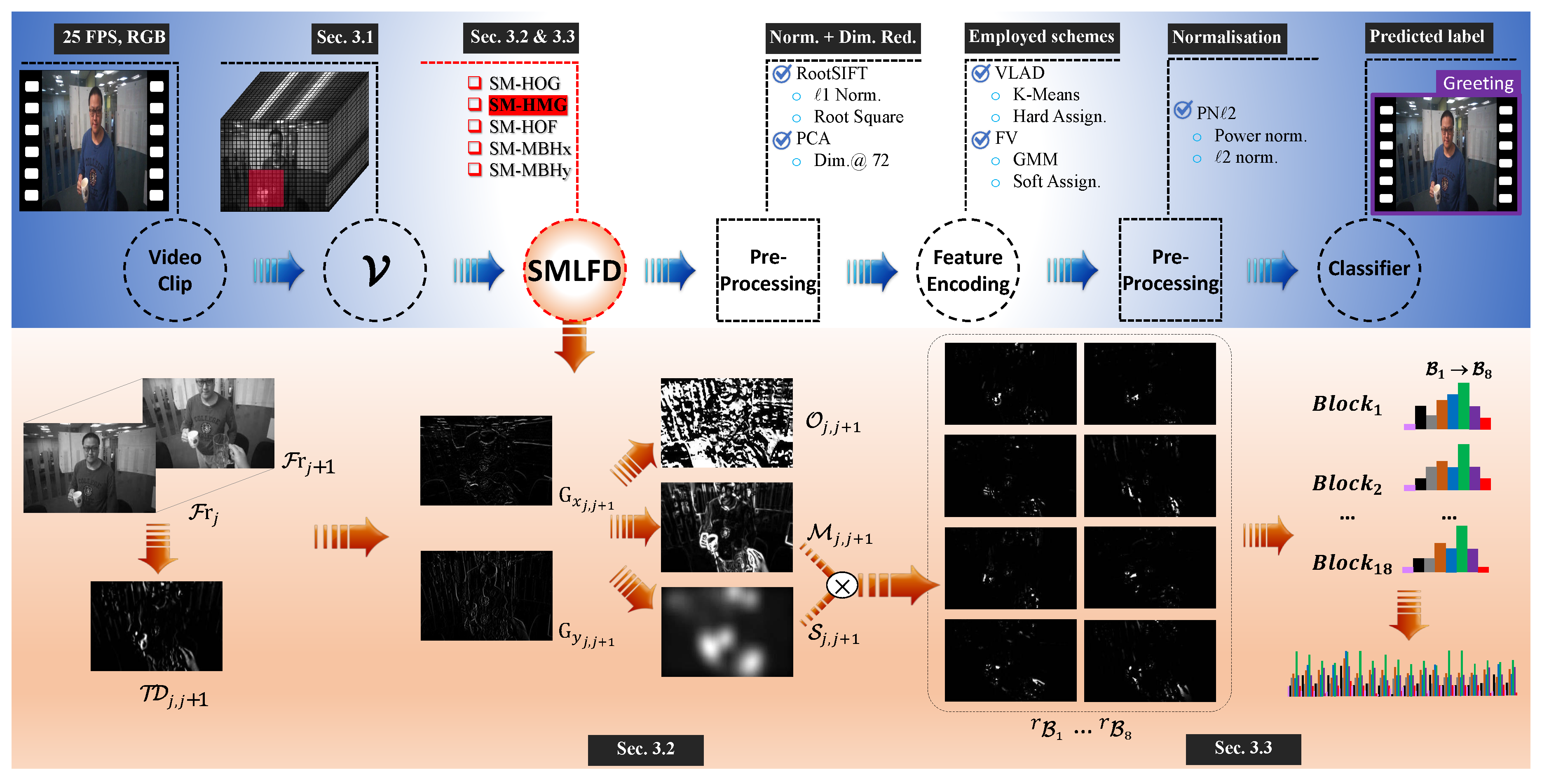
The framework of the proposed saliency map-based egocentric action recognition is illustrated in Figure 1, which highlights the proposed SMLFD feature extraction approach itself, as detailed in Section 3.3. This framework was developed according to the principle of the BoVW approach. In the illustrative diagram, SM-HMG is used as a representative example to demonstrate the workflow of the proposed approach, as shown in the bottom row of Figure 1. In particular, the SM-HMG feature extraction approach takes two consecutive frames in a 3D video matrix as the input. Then, the motion information between the two consecutive frames () is captured via a temporal derivative operation with respect to time t. This is followed by the calculation of gradients in the spatial x and y directions. From this, the magnitudes and orientations of every pixel in the frame are calculated (frame-wise, jointly denoted as and ), thus generating the corresponding saliency map . Then, the magnitude response of pixels are aggregated into a limited number of evenly divided directions over 2, i.e., bins. In this illustrative example, eight bins are used. This is followed by a weighting operation using saliency information to generate a histogram of bins for each block. The final feature representation is then generated by concatenating all the block information (18 blocks in this illustrative example) into a holistic histogram feature vector. The key steps of this process are presented in the following subsections. The processes of feature encoding [5,6,7,32], pre- and post-processing [8,14,35,39], and classification [5,6,9,14] are omitted here as they are not the focus of this work, but these topics have been intensively studied and are available in the literature.
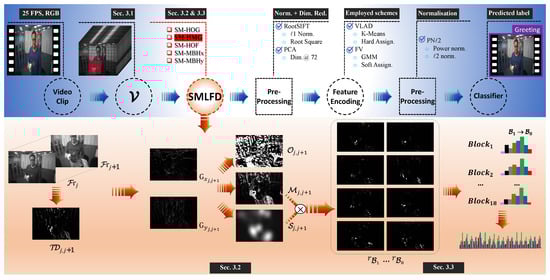
Figure 1.
The framework of the proposed approach as shown in the upper row, and the outline of the main steps of the saliency map-enhanced LFD extraction approach (SMLFD) as illustrated in the lower row using the histogram of motion gradients (HMG) approach with 8 bins and 18 blocks.
3.1. Video Representation
An egocentric video clip is usually formed by a set of video frames, and each frame is represented as a two-dimensional array of pixels. Thus, each video clip can be viewed as a three-dimensional array of pixels, with x- and y-axes representing the plane of the video frame, and the t-axis denoting the timeline. An egocentric video clip is denoted by , where represents the resolution of each video frame, and f represents the total number of frames. Histogram-based LFDs use each pair of consecutive frames and to capture the motion information along the timeline (except HOG, which does not consider the temporal information) and use the neighboring pixels in every frame to extract the spatial information. In this work, all LFDs, including HOG, HMG, HOF, MBHx, and MBHy, were enhanced by using the saliency map, yielding SM-HOG, SM-HMG, SM-HOF, SM-MBHx, and SM-MBHy, respectively. Briefly, HOG, HMG, HOF, and MBH represent videos using the in-frame gradient only, in-and-between frame gradient, in-frame optical flow and between-frame gradient, and the imaginary and real parts of the optical flow gradient and between-frame gradient, respectively.
3.2. Local Spatial and Temporal Information Calculation
SM-HOG and SM-HMG: SM-HOG calculates spatial gradient information for each input video frame . By extending SM-HOG, SM-HMG performs an efficient temporal gradient calculation between each pair of neighboring frames () prior to the entire SM-HOG process using Equation (1).
The gradients in the x and y directions for SM-HOG, SM-HMG, SM-HBHx, and SM-MBHy are summarized below:
where and for SM-HOG, and and for the others. Please note that the above derivative operations are usually practically implemented using a convolution with a Haar kernel [41]. Then, the magnitude and orientation of the temporal and spatial information about the pixels in each frame are calculated as:
where |·| and denote the magnitude and orientation of the complex-typed vector, respectively.
3.3. Saliency Map-Informed Bin Response Generation
The orientations of temporal and spatial information are evenly quantized into b bins in the range of [0, 2], i.e., , , to aggregate the gradient information of pixels. The original LFD methods assign the two closest bins to each pixel on the basis of its gradient orientation, and the bin strength of each of these is calculated as the weighted summation of the magnitude of the bin’s partially assigned pixels. Given pixel p in frame with gradient orientation and magnitude , which are calculated using Equation (3), suppose that the two neighboring bins are and . Then, the weights of pixel p relative to and are calculated as and , respectively. From this, the contributions of pixel p to bins and are calculated as and , respectively.
Given that a saliency map represents the visual attractiveness of a frame, the saliency values are essentially a fuzzy distribution of each pixel regarding its visual attractiveness. Therefore, the saliency membership of each pixel p indicates its importance to the video frame from the perspective of human visual attention. On the basis of this observation, this work further distinguished the contribution of each pixel to its neighboring bins by introducing the saliency membership to the bin strength calculation. In particular, the weights and of pixel p relative to its neighboring bins and are updated by the aggregation of its saliency membership value; that is, the original weights and are updated to and . Accordingly, the contributions of pixel p to bins and are updated as and , respectively.
There are multiple ways available in the literature for the calculation of saliency maps. This work adopted the approach reported in [15], which is a pixel-based saliency membership generation approach proposed according to the hypothesis that the most important part or parts of an image are in the foreground. The pseudo-code of the algorithm is illustrated in Algorithm 1. The saliency map of a frame is denoted by S, which collectively represents the saliency value of every pixel p in the frame. Briefly, each frame is first converted to three color channels, Red, Green, and Blue (RGB), denoted by , as shown in Line 1 of the algorithm. Then, the video frame in RGB is converted to the CIELAB space with L, A, and B channels [42], as indicated by Line 2. This is followed by reconstructing the frame using discrete cosine transform (DCT) The D(·) operation and inverse DCT D[·] operation in Line 3 distinguish the foreground and background in a fuzzy way. From this, in Line 4, the mean values of the pixels in the L, A, B channels are computed and denoted as ; the surface is smoothed via a Gaussian kernel with the entry-wise Hadamard product (i.e., ∘) operation, with output . The final saliency map S is then obtained by normalizing each value in to the range of .
| Algorithm 1: Saliency Membership Calculation Procedure. |
| Input: : the ith 2D video frame, Output: S: saliency membership of the ith frame Procedure getSaliencyMap
|
The extra computational complexity of the proposed approach, compared with the original versions, mainly lies in the calculation of the saliency map, as the saliency information is integrated into the proposed approach by a simple multiplication operation. The computational cost of the saliency map approach used in this work is generally moderate, as it is only a fraction of the cost of other saliency algorithms [15].
4. Experiments and Results
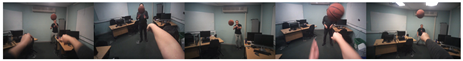
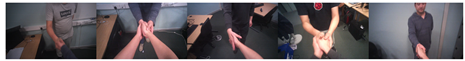
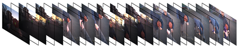
As described in this section, the publicly available video dataset UNN-GazeEAR [5] was utilized to evaluate the performance of the proposed methods, with the support of a comparative study in reference to the GROILFD approach [5]. The UNN-GazeEAR dataset consists of 50 video clips in total, including five egocentric action categories. The length of the videos ranges from 2 to 11 seconds, with 25 frames per second. The sample frames are shown in Table 1. All the experiments were conducted using an HP workstation with Intel® Xeon™ E5-1630 v4 CPU @ 3.70 GHz and 32 GB RAM.

Table 1.
Illustrative frames of the UNN-GazeEAR dataset.
4.1. Experimental Setup
The parameters used in [5,6,9,14,35,39] were also adopted in this work. Specifically, the BoVW model and PCA were employed to select 72 features. The value of the normalization parameter of PNℓ2 was fixed to 0.5. A back-propagation neural network (BPNN) was used for classification after the features were extracted. The BPNN was trained using the scaled conjugate gradient (SCG) algorithm with a maximum of 100 training epochs. The number of neurons in the hidden layer was fixed to 20, and the training ratio was set to 70%. The performance metric was the mean accuracy of 100 independent runs.
4.2. Experiments with Different Resolutions, Block Sizes, and Feature Encoding Methods
In this experiment, SMLFD (including SM-HOG, SM-HMG, SM-HOF, SM-MBHx, and SM-MBHy) was applied for comparison with GROILFD [5] (covering GROI-HOG, GROI-HMG, GROI-HOF, GROI-MBHx, and GROI-MBHy). Videos with the same down-scaled resolution (by a factor of 6), as reported in [5], were used in this experiment as the default. Thus, each video in the dataset has a uniform resolution of 320 × 180 pixels.
Firstly, the values of the feature extraction time were studied. Table 2 and Table 6 show the speed of extracting SMLFD was significantly boosted by at least 40-fold (denoted as 40×). When using a block size of 16-by-16 spacial pixels by 6 temporal frames (denoted as [16 × 16 × 6]) for the feature extraction, SM-HOG, SM-HMG, SM-HOF, SM-MBHx, and SM-MBHy were boosted by 40×, 41×, 43×, 41×, and 41×, respectively. When using a block size of [32 × 32 × 6], SM-HOG, SM-HMG, SM-HOF, SM-MBHx, and SM-MBHy were boosted by 41×, 43×, 45×, 43×, and 43×, respectively. Because GROILFD extracts the sparse features, SMLFD feature extraction needs more computational time than GROILFD. However, VLAD and FV feature encoding methods consume similar amounts of time for feature encoding.
Table 2.
Comparison of different feature descriptors under down-scaled resolution.
In terms of accuracy, the performance of SMLFD was improved significantly compared with that using the original resolution. Furthermore, SMLFD consistently outperformed GROILFD with the down-scaled dataset, because SMLFD constructed dense features. To investigate the trade-off between performance and time complexity, the features encoded with a smaller number of visual words were studied. Table 2 shows that SMLFD generally had better accuracy when using smaller block sizes (i.e., [4 × 4 × 6], [8 × 8 × 6], and [16 × 16 × 6]), while GROILFD outperformed when using larger ones. Therefore, this indicates that SMLFD is a better candidate for low-resolution videos.
4.3. Experiments with Varying Number of Visual Words for Encoding
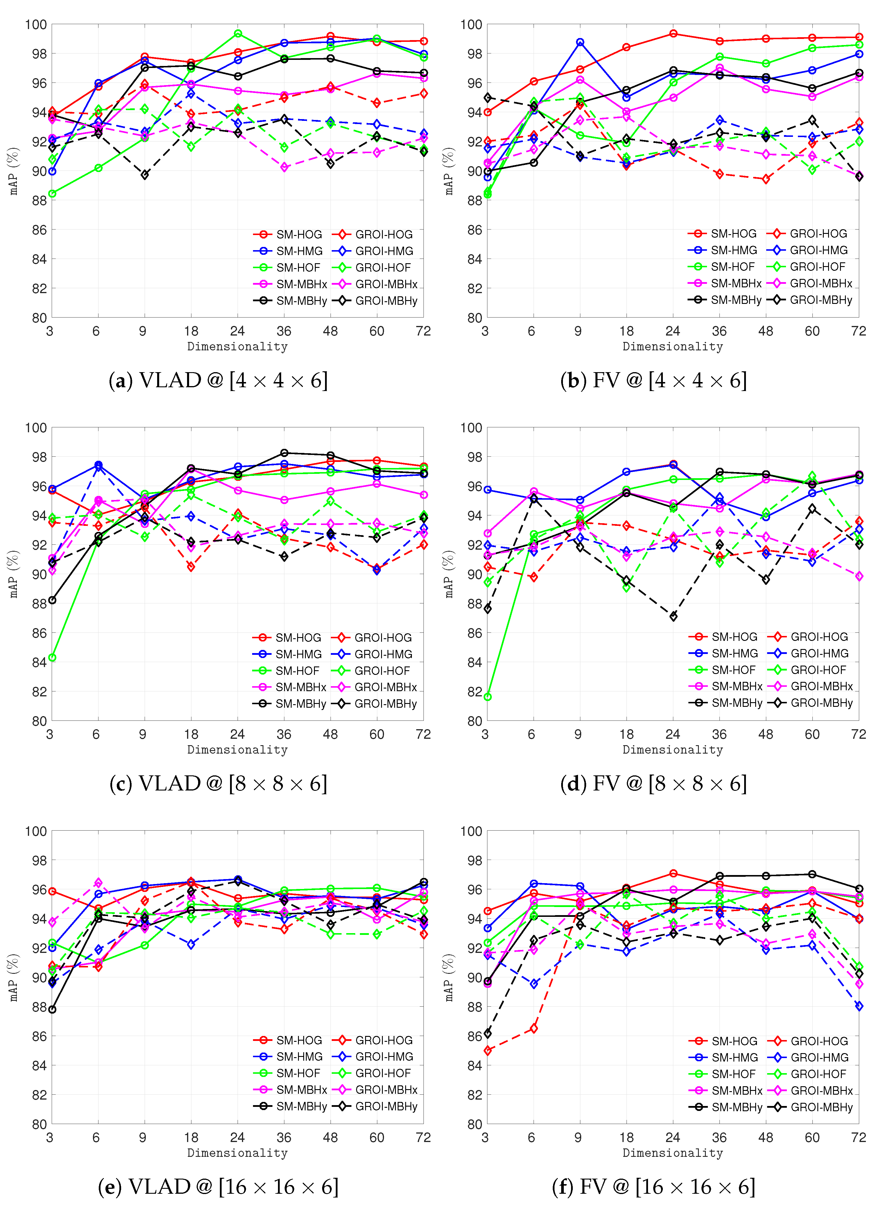
In this experiment, the effect of varying the number of visual words used in the VLAD and FV feature encoding scheme was investigated. Specifically, half of the visual words were used to compare with the setting in the experiment reported in Section 4.2. The impact of feature dimensions was also investigated when using PCA in the preprocessing phase. The results are shown in Figure 2. The experiment used 3, 6, 9, 18, 24, 36, 48, 60, and 72 feature dimensions. SMLFD outperformed GROILFD when using a small number of visual words for feature encoding. The best performances that were achieved by SMLFD are summarized in Table 3. As shown in Figure 3, SM-HOG exceeded other approaches in most cases when using block sizes of and . However, SM-HMG outperformed others in most cases for a block size of .
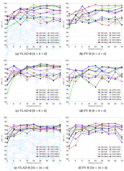
Figure 2.
Performance comparison between local features with different feature dimensions.
Table 3.
Accuracy comparison of saliency map-enhanced local feature descriptors (SMLFDs) using different feature dimensions with various block sizes (the adopted color schemes are consist with Figure 2).
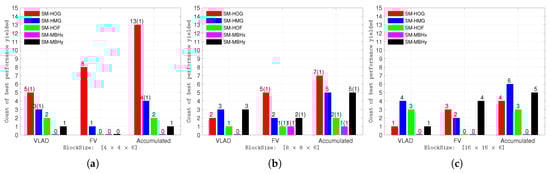
Figure 3.
Statistics of the best performance obtained for each employed block size. (·) denotes the number of best performances that were equivalently achieved by other feature descriptors in the SMLFD family. (a) ; (b) ; (c) .
Table 4 shows that the proposed SMLFD outperformed GROILFD. SMLFD achieved its peak performance when using a smaller block size (i.e., [4 × 4 × 6]) while GROILFD reached its best performance when using a larger block size [16 × 16 × 6] with VLAD and [8 × 8 × 6] with FV). This again indicates that SMLFD and GROILFD represent families of local dense feature descriptors and sparse feature descriptors, respectively.
Table 4.
Comparison of the top performing feature descriptor with that of the other feature descriptors for different feature encoding schemes on the UNN-GazeEAR dataset. The global best accuracies in both (SMLFD and GROILFD) are marked with gray color.
4.4. Experiment Using the Memory Aid Dataset
In this experiment, the trained models (with which the SMLFD features were extracted) were applied to an untrimmed video stream that was published in [5]. Table 5 shows that the SMLFD-trained models possessed better performance compared with that trained using GROILFD features. In general, SMLFD performed as well as GROILFD. Each of them had three superior performances and four equivalent performances. Similarly, both SM-HOG and GROI-HOG achieved 100% accuracy using FV feature encoding. The three higher results yielded by GROILFD were produced by GROI-HOG, GROI-MBHx, and GROI-MBHy, all under VLAD feature encoding.
Table 5.
Testing video stream for the memory aid system with five activities of daily living (ADLs).
4.5. Comparison with Original Resolution
The proposed SMLFD family of local feature descriptors can achieve comparable results to GROILFD. In this experiment, the proposed SMLFD feature descriptors were investigated by adopting all videos from the dataset with the original resolution of 1920 × 1080 pixels. Given the comparison results in Table 6, GROILFD clearly outperformed SMLFD in terms of accuracy and required time for feature extraction. The reason for this is threefold: (1) GROILFD only proceeds with a single connected interest region with the noise removed from the frame, whereas SMLFD deals with all the pixels in each frame; thus, GROILFD is a faster family of feature extraction approaches; (2) SMLFD extends LFD by introducing an additional real-time operation of calculating the frame-wise saliency membership with a high degree of sensitivity to the resolution of the video; (3) SMLFD is not efficient in suppressing irrelevant background and foreground noises. To conclude, SMLFD is highly scale-variant and GROILFD is a better candidate for videos with high resolution.
Table 6.
Comparison with other feature descriptors.
4.6. Discussion
Egocentric videos are usually non-stationary due to the camera motion of the smart glasses or other data-capturing devices; the experimental results of using the proposed local features indicate the ability of the proposed approach to cope with this challenge during video action recognition. Of course, the proposed feature descriptors also have their own limitations. For instance, the computation cost of the proposed approach is generally higher than that of the originals. Also, the performance of the proposed approach closely depends on the accuracy of the calculated saliency map, and poorly generated saliency maps may significantly limit the effectiveness of the proposed approach. Of course, there is a good selection of approaches available in the literature for saliency map calculation, and their effectiveness in supporting the proposed approach requires further investigation.
5. Conclusions
This paper proposes a family of novel saliency-informed local feature descriptor extraction approaches for egocentric action recognition. The performance of the proposed family of feature descriptors was evaluated using the UNN-GazeEAR dataset. The experimental results demonstrate the effectiveness of the proposed method in improving the performance of the original LFD approaches. This indicates that the saliency map can be a useful ingredient for extracting local spatial and temporal features in the recognition of first-person video actions. Possible future work includes more large-scale applications, which are required to further evaluate the proposed approach. It would also be interesting to investigate how the saliency map can support global feature descriptors. Another interesting potential investigation would be broadening the applicability of the proposed feature descriptors for object detection using an electromagnetic source [43,44,45] (e.g., signals, pictures of vehicles, antennas, etc.).
Author Contributions
Conceptualization, L.Y. and Z.Z.; methodology, Z.Z., F.C. and Y.Q.; software, Z.Z.; validation, L.Y., B.W. and Y.P.; writing–original draft preparation, Z.Z.; writing–review and editing, B.W., F.C., Y.Q., Y.P., and L.Y.; supervision, L.Y.
Funding
This research received no external funding.
Conflicts of Interest
The authors declare no conflict of interest.
Abbreviations
The following abbreviations are used in this manuscript:
| BoVW | Bag of Visual Words |
| LFD | Local Feature Descriptors |
| SMLFD | Saliency Membership based Local Feature Descriptors |
| SM-HOG | Saliency Membership based Histogram of Oriented Gradients |
| SM-HMG | Saliency Membership based Histogram of Motion Gradients |
| SM-HOF | Saliency Membership based Histogram of Optical Flow |
| SM-MBHx | Saliency Membership based Motion Boundary Histogram (in x direction) |
| SM-MBHy | Saliency Membership based Motion Boundary Histogram (in y direction) |
| GROILFD | Gaze Region of Interest based Local Feature Descriptors |
| GROI-HOG | Gaze Region of Interest based Histogram of Oriented Gradients |
| GROI-HMG | Gaze Region of Interest based Histogram of Motion Gradients |
| GROI-HOF | Gaze Region of Interest based Histogram of Optical Flow |
| GROI-MBHx | Gaze Region of Interest based Motion Boundary Histogram (in x direction) |
| GROI-MBHy | Gaze Region of Interest based Motion Boundary Histogram (in y direction) |
References
- Betancourt, A.; Morerio, P.; Regazzoni, C.S.; Rauterberg, M. The Evolution of First Person Vision Methods: A Survey. IEEE Trans. Circ. Syst. Video Technol. 2015, 25, 744–760. [Google Scholar] [CrossRef]
- Nguyen, T.H.C.; Nebel, J.C.; Florez-Revuelta, F. Recognition of activities of daily living with egocentric vision: A review. Sensors 2016, 16, 72. [Google Scholar] [CrossRef] [PubMed]
- Zaki, H.F.M.; Shafait, F.; Mian, A. Modeling Sub-Event Dynamics in First-Person Action Recognition. In Proceedings of the IEEE Conference on Computer Vision and Pattern Recognition (CVPR 2017), Honolulu, HI, USA, 21–26 July 2017; pp. 1619–1628. [Google Scholar]
- Fan, C.; Lee, J.; Xu, M.; Singh, K.K.; Lee, Y.J.; Crandall, D.J.; Ryoo, M.S. Identifying First-Person Camera Wearers in Third-Person Videos. In Proceedings of the IEEE Conference on Computer Vision and Pattern Recognition (CVPR 2017), Honolulu, HI, USA, 21–26 July 2017; pp. 4734–4742. [Google Scholar]
- Zuo, Z.; Yang, L.; Peng, Y.; Chao, F.; Qu, Y. Gaze-Informed Egocentric Action Recognition for Memory Aid Systems. IEEE Access 2018, 6, 12894–12904. [Google Scholar] [CrossRef]
- Zuo, Z.; Organisciak, D.; Shum, H.P.H.; Yang, L. Saliency-Informed Spatio-Temporal Vector of Locally Aggregated Descriptors and Fisher Vectors for Visual Action Recognition. In Proceedings of the British Machine Vision Conference (BMVC 2018), Newcastle, UK, 2–6 September 2018; p. 321. [Google Scholar]
- Jegou, H.; Perronnin, F.; Douze, M.; Sánchez, J.; Pérez, P.; Schmid, C. Aggregating local image descriptors into compact codes. IEEE Trans. Pattern Anal. Mach. Intell. 2012, 34, 1704–1716. [Google Scholar] [CrossRef] [PubMed]
- Wang, H.; Schmid, C. Action recognition with improved trajectories. In Proceedings of the IEEE International Conference on Computer Vision (ICCV 2013), Sydney, NSW, Australia, 1–8 December 2013; pp. 3551–3558. [Google Scholar]
- Cameron, R.; Zuo, Z.; Sexton, G.; Yang, L. A Fall Detection/Recognition System and an Empirical Study of Gradient-Based Feature Extraction Approaches. In UKCI 2017: Advances in Computational Intelligence Systems; Chao, F., Schockaert, S., Zhang, Q., Eds.; Advances in Intelligent Systems and Computing; Springer: Cham, Switzerland, 2017; Volume 650, pp. 276–289. [Google Scholar]
- Sivic, J.; Zisserman, A. Video Google: A text retrieval approach to object matching in videos. In Proceedings of the IEEE International Conference on Computer Vision (ICCV 2003), Nice, France, 13–16 October 2003; pp. 1470–1477. [Google Scholar]
- Dalal, N.; Triggs, B. Histograms of oriented gradients for human detection. In Proceedings of the IEEE Conference on Computer Vision and Pattern Recognition (CVPR 2005), San Diego, CA, USA, 20–25 June 2005; pp. 886–893. [Google Scholar] [CrossRef]
- Laptev, I.; Marszalek, M.; Schmid, C.; Rozenfeld, B. Learning realistic human actions from movies. In Proceedings of the IEEE Conference on Computer Vision and Pattern Recognition (CVPR), Anchorage, AK, USA, 23–28 June 2008. [Google Scholar] [CrossRef]
- Dalal, N.; Triggs, B.; Schmid, C. Human Detection Using Oriented Histograms of Flow and Appearance. In Proceedings of the European Conference on Computer Vision (ECCV 2006), Graz, Austria, 7–13 May 2006; pp. 428–441. [Google Scholar]
- Duta, I.C.; Uijlings, J.R.R.; Nguyen, T.A.; Aizawa, K.; Hauptmann, A.G.; Ionescu, B.; Sebe, N. Histograms of motion gradients for real-time video classification. In Proceedings of the IEEE International Workshop on Content-Based Multimedia Indexing (CBMI 2016), Bucharest, Romania, 15–17 June 2016. [Google Scholar] [CrossRef]
- Hou, X.; Harel, J.; Koch, C. Image signature: Highlighting sparse salient regions. IEEE Trans. Pattern Anal. Mach. Intell. 2012, 34, 194–201. [Google Scholar]
- Liu, B.; Ju, Z.; Liu, H. A structured multi-feature representation for recognizing human action and interaction. Neurocomputing 2018, 318, 287–296. [Google Scholar] [CrossRef]
- Laptev, I. On Space-Time Interest Points. Int. J. Comput. Vision (IJCV) 2005, 64, 107–123. [Google Scholar] [CrossRef]
- Dollar, P.; Rabaud, V.; Cottrell, G.; Belongie, S. Behavior recognition via sparse spatio-temporal features. In Proceedings of the 2005 IEEE International Workshop on Visual Surveillance and Performance Evaluation of Tracking and Surveillance (VS-PETS), Beijing, China, 15–16 October 2005; pp. 65–72. [Google Scholar]
- Lowe, D.G. Distinctive Image Features from Scale-Invariant Keypoints. Int. J. Comput. Vision (IJCV) 2004, 60, 91–110. [Google Scholar] [CrossRef]
- Mikolajczyk, K.; Schmid, C. A performance evaluation of local descriptors. IEEE Trans. Pattern Anal. Mach. Intell. (TPAMI) 2005, 27, 1615–1630. [Google Scholar] [CrossRef] [PubMed]
- Bay, H.; Tuytelaars, T.; Van Gool, L. Surf: Speeded up robust features. In Proceedings of the European Conference on Computer Vision (ECCV 2006), Graz, Austria, 7–13 May 2006; pp. 404–417. [Google Scholar]
- Scovanner, P.; Ali, S.; Shah, M. A 3-dimensional sift descriptor and its application to action recognition. In Proceedings of the ACM International Conference on Multimedia (ACMMM), Augsburg, Germany, 24–29 September 2007; pp. 357–360. [Google Scholar]
- Bay, H.; Ess, A.; Tuytelaars, T.; Van Gool, L. Speeded-up robust features (SURF). Comput. Vis. Image Und. 2008, 110, 346–359. [Google Scholar] [CrossRef]
- Fathi, A.; Mori, G. Action recognition by learning mid-level motion features. In Proceedings of the IEEE Conference on Computer Vision and Pattern Recognition (CVPR 2008), Anchorage, AK, USA, 23–28 June 2008. [Google Scholar] [CrossRef]
- Sadanand, S.; Corso, J.J. Action bank: A high-level representation of activity in video. In Proceedings of the IEEE Conference on Computer Vision and Pattern Recognition (CVPR 2012), Providence, RI, USA, 16–21 June 2012; pp. 1234–1241. [Google Scholar]
- Wang, S.; Hou, Y.; Li, Z.; Dong, J.; Tang, C. Combining convnets with hand-crafted features for action recognition based on an HMM-SVM classifier. Multimed. Tools Appl. 2016, 77, 18983–18998. [Google Scholar] [CrossRef]
- Hassner, T. A critical review of action recognition benchmarks. In Proceedings of the IEEE Conference on Computer Vision and Pattern Recognition Workshops (CVPRW 2013), Portland, OR, USA, 23–28 June 2013; pp. 245–250. [Google Scholar]
- Borji, A.; Cheng, M.M.; Jiang, H.; Li, J. Salient Object Detection: A Benchmark. IEEE Trans. Image Process. 2015, 24, 5706–5722. [Google Scholar] [CrossRef] [PubMed]
- Nguyen, T.V.; Song, Z.; Yan, S. STAP: Spatial-Temporal Attention-Aware Pooling for Action Recognition. IEEE Trans. Circ. Syst. Video Technol. 2015, 25, 77–86. [Google Scholar] [CrossRef]
- Huang, Y.; Huang, K.; Yu, Y.; Tan, T. Salient coding for image classification. In Proceedings of the IEEE Conference on Computer Vision and Pattern Recognition (CVPR 2011), Colorado Springs, CO, USA, 20–25 June 2011; pp. 1753–1760. [Google Scholar]
- Wang, J.; Yang, J.; Yu, K.; Lv, F.; Huang, T.; Gong, Y. Locality-constrained linear coding for image classification. In Proceedings of the IEEE Conference on Computer Vision and Pattern Recognition (CVPR 2010), San Francisco, CA, USA, 13–18 June 2010; pp. 3360–3367. [Google Scholar]
- Perronnin, F.; Sánchez, J.; Mensink, T. Improving the Fisher Kernel for Large-scale Image Classification. In Proceedings of the European Conference on Computer Vision (ECCV 2010), Crete, Greece, 5–11 September 2010; pp. 143–156. [Google Scholar]
- Van Der Maaten, L.; Postma, E.; Van den Herik, J. Dimensionality reduction: a comparative. J. Mach. Learn. Res. 2009, 10, 66–71. [Google Scholar]
- Zuo, Z.; Li, J.; Anderson, P.; Yang, L.; Naik, N. Grooming detection using fuzzy-rough feature selection and text classification. In Proceedings of the 2018 IEEE International Conference on Fuzzy Systems (FUZZ-IEEE), Rio de Janeiro, Brazil, 8–13 July 2018. [Google Scholar]
- Uijlings, J.; Duta, I.C.; Sangineto, E.; Sebe, N. Video classification with Densely extracted HOG/HOF/MBH features: An evaluation of the accuracy/computational efficiency trade-off. Int. J. Multimed. Inf. Retr. 2015, 4, 33–44. [Google Scholar] [CrossRef]
- Iosifidis, A.; Tefas, A.; Pitas, I. View-Invariant Action Recognition Based on Artificial Neural Networks. IEEE Trans. Neural Netw. Learn. Syst. 2012, 23, 412–424. [Google Scholar] [CrossRef] [PubMed]
- Zhou, Y.; Yu, H.; Wang, S. Feature sampling strategies for action recognition. In Proceedings of the IEEE International Conference on Image Processing (ICIP 2017), Beijing, China, 17–20 September 2017; pp. 3968–3972. [Google Scholar]
- Lazebnik, S.; Schmid, C.; Ponce, J. Beyond bags of features: Spatial pyramid matching for recognizing natural scene categories. In Proceedings of the IEEE Conference on Computer Vision and Pattern Recognition (CVPR’06), New York, NY, USA, 17–22 June 2006; Volume 2, pp. 2169–2178. [Google Scholar]
- Peng, X.; Wang, L.; Wang, X.; Qiao, Y. Bag of visual words and fusion methods for action recognition: Comprehensive study and good practice. Comput. Vis. Image Und. 2016, 150, 109–125. [Google Scholar] [CrossRef]
- Horn, B.K.; Schunck, B.G. Determining optical flow. Artif. Intell. 1981, 17, 185–203. [Google Scholar] [CrossRef]
- Viola, P.; Jones, M. Rapid object detection using a boosted cascade of simple features. In Proceedings of the IEEE Conference on Computer Vision and Pattern Recognition (CVPR 2001), Kauai, HI, USA, 8–14 December 2001; Volume 1, pp. 511–518. [Google Scholar]
- Zhang, X.; Wandell, B.A. A spatial extension of CIELAB for digital color-image reproduction. J. Soc. Inf. Display 1997, 5, 61–63. [Google Scholar] [CrossRef]
- Kawalec, A.; Rapacki, T.; Wnuczek, S.; Dudczyk, J.; Owczarek, R. Mixed method based on intrapulse data and radiated emission to emitter sources recognition. In Proceedings of the IEEE International Conference on Microwave Radar and Wireless Communications (MIKON 2006), Krakow, Poland, 22–24 May 2006; pp. 487–490. [Google Scholar]
- Matuszewski, J. The radar signature in recognition system database. In Proceedings of the IEEE International Conference on Microwave Radar and Wireless Communications (MIKON 2012), Warsaw, Poland, 21–23 May 2012; Volume 2, pp. 617–622. [Google Scholar]
- Matuszewski, J.; Sikorska-Łukasiewicz, K. Neural network application for emitter identification. In Proceedings of the IEEE International Radar Symposium (IRS 2017), Prague, Czech Republic, 28–30 June 2017. [Google Scholar] [CrossRef]


© 2019 by the authors. Licensee MDPI, Basel, Switzerland. This article is an open access article distributed under the terms and conditions of the Creative Commons Attribution (CC BY) license (http://creativecommons.org/licenses/by/4.0/).