Article

Optimal Fuel Consumption Modelling, Simulation, and Analysis for Hybrid Electric Vehicles

1
Institute for Nanomaterials, Advanced Technologies and Innovation, Technical University of Liberec, 461 17 Liberec, Czech Republic
2
Faculty of Mechatronics, Informatics and Interdisciplinary Studies, Technical University of Liberec, 461 17 Liberec, Czech Republic
*
Author to whom correspondence should be addressed.
Appl. Syst. Innov. 2022, 5(2), 36; https://doi.org/10.3390/asi5020036
Submission received: 1 December 2021 / Revised: 17 January 2022 / Accepted: 28 February 2022 / Published: 10 March 2022

Abstract

:
This paper reviews the latest studies of hybrid electric vehicles (HEVs) on modelling, controls, and energy management. HEV dynamics, formulas, calculations, and schemes of vehicle parts, such as battery, converter, electric motor, generator, and HEV Simulink models, are presented. Moreover, simulations of the propulsion operation, regenerative braking system, and vehicle dynamics are conducted. A comprehensive HEV model is built that is simulated on different driving cycles of Federal Test Procedure 75 (FTP75), New York City Cycle (NYCC), Highway Fuel Economy Test (HWFET), and Extra Urban Driving Cycle (EUDC). Data achieved from these simulations were analysed and tested with several fuel regression models to determine the best fuel regression estimation for HEV fuel consumption on the basis of their weights and tire radiuses. The best fuel regression equation is obtained with a determination coefficient R-squared greater than 99%. Lastly, the optimal model and other HEVs models are simulated on different driving cycles to prove that the fuel consumption of our best-fit regression model is the best.

1. Introduction

Hybrid electric vehicles (HEVs) have been increasingly popular since the global commitment to restrain the use of fossil fuels and to limit CO2 emissions. HEVs help to save fuel consumption and reduce CO2 emissions by less than 50% of conventional vehicles using only internal combustion engines (ICEs). In the future, electric vehicles (EVs) may replace ICEs, but EVs still have serious problems of high costs, limited range, and long-term charging. Therefore, HEVs can overcome all the disadvantages of both ICEs and EVs since HEVs are the combination of the advantages of both ICEs and EVs, with broad range, low emissions, high fuel efficiency, high reliability, and low costs. In 2021, roughly 10 million HEVs were globally produced and sold. HEV production is projected to reach 100 million by 2050. A comprehensive review on the state of the art and trends in HEVs was reported in [1]. Another systematic review of the recent technologies, control methods, and energy optimization managers for HEVs was presented in [2].
In reviewing recent HEV energy management and optimal control, the authors in [3] provided an in-depth literature review on vehicle fuel consumption and emission modelling to predict vehicle fuel consumption and emissions. The authors in [4] presented another comprehensive review on the control of HEV transmissions and powertrains, including automated manual transmission (AMT), manual transmission (MT), and dual-clutch transmission (DCT). Another comprehensive review on HEV architectures and components was introduced in [5] for modern HEVs. The authors in [6] presented the recent advances of HEVs in relation to fuel-saving performance and energy management strategy. In [7], the authors conducted a closer review on HEV driveline lubrication to improve fuel efficiency and reduce emissions. Another review article on power management and control for HEVs was presented in [8]. A review of the HEV energy management strategy depending on road condition information was introduced in [9]. Lastly, recent progress on the HEV perspective on fuel management was presented in [10].
In reviewing the development trends of HEV powertrains and transmissions, the authors in [11] introduced updated trends of HEVs using optimal energy management. The authors in [12] investigated the effect of clutch slip losses and combustion engine start on the fuel management problem. In [13], the authors studied the modelling and fuel management of powertrain split on HEVs. Six operation modes of the vehicles were discussed for the impact of different fuel management strategies on energy and energy efficiency analysis were presented in [14]. The authors in [15] studied the efficiency optimization of regenerative braking systems for HEVs. Lastly, the authors in [16] conducted simulations of full HEVs running on standard driving cycles and the Urban Dynamometer Driving Schedule (UDDS).
Reviewing the control strategy for HEVs, the authors in [17] presented control strategies for HEVs depending on different online driving patterns. This study investigates the feasibility of optimising control for different driving patterns, so that the vehicle can maintain a high level of optimality regardless of the driving pattern. Another control strategy for clutch engagement during mode changing for HEVs was presented in [18]. The authors in [19] present mode transition control for single shaft parallel HEVs using a model predictive control. This optimal control strategy can be achieved by using quadratic programming in the infinite prediction horizon. The authors in [20] conducted research on the multiphase mixed integer nonlinear optimal control of HEVs for a minimal fuel energy management strategy. Lastly, the authors in [21] presented the economic aspect of different HEVs in urban conditions to reduce fuel consumption and shorten travelling time.
Recent studies on modelling fuel consumption for HEVs were reviewed. The authors in [22] conducted research on HEV benefits to improve the fuel economy and reduce emissions. Trends in the design, energy management, component sizing, fuel cost, and performance of HEVs are presented and analysed. A case study for HEV energy consumption modelling and estimation is presented in [23], where a driver model was set up to control the vehicle and represent human behaviour. Lastly, a proposal to accurately estimate the fuel consumption of HEVs, depending on real-world data consisting of instantaneous energy consumption, time variation in speed, and high-frequency traffic, was presented in [24].
Recent reviews on optimal fuel management still lack an optimal estimation of HEV fuel consumption depending on the size and tires. Therefore, this paper attempts to discover the elements that affect the fuel consumption and determines the best HEV model with sizes and tires for achieving the best fuel consumption. This paper is organised as follows: Section 2 presents HEV drivetrain modelling; Section 3 presents HEV scheme simulations; Section 4 presents fuel economy modelling and regressions; and, lastly, Section 5 draws the conclusions. In this paper, most HEV dynamics, modelling, calculations, energy equations, and simulation schemes refer to our textbook [25] and to [26,27]. The updated Internet sources for different HEVs used in the online references are [28,29,30,31,32,33,34,35]. The latest mathematical formulations are referred to in [36,37,38,39].

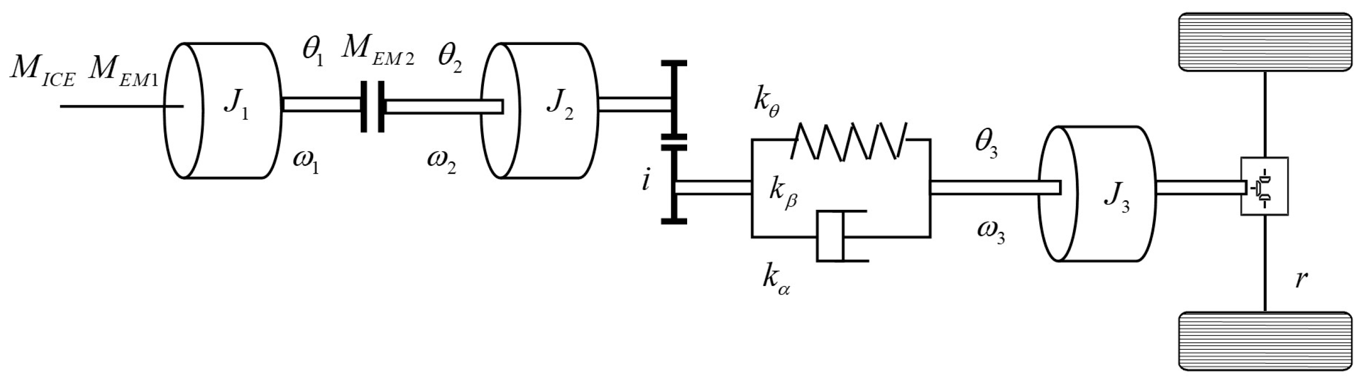
2. HEV Powertrain Modelling

HEVs usually have two power sources: a combustion engine and an electrical motor with a large battery to run the vehicle. A typical HEV has a parallel HEV scheme for which the internal combustion engine (ICE) and the main electrical motor (EM2) are installed parallelly and independently, so that the HEV can run in four driving modes (DMs). At a low speed and/or low load, only the main EM2 propels the vehicle (pure electric mode or DM1). At a higher speed and/or higher load, the ICE is started by a starter/generator electric motor (EM1) and propels the vehicle (pure ICE mode or DM2); EM1 is turned off or becomes the generator to charge the battery. At a very high speed or very high load, the vehicle is run by both EM2 and ICE (hybrid mode or DM3). Lastly, at an extreme high speed and/or extreme high load, EM2, EM1, and ICE together run the vehicle (extreme hybrid mode or DM4). The vehicle battery can be charged offline from a plug-in cable or online by an EM1 generator when necessary.
Hyundai launched the latest version of the Sonata Hybrid in 2021. This is a typical sedan middle-class parallel HEV. This HEV consists of 1 ICE with 4 cylinders of multiple point injections, a displacement of 2.4 litters, maximum power of 156 kW at 6000 rpm, and a peak torque of 256 N m; 1 main EM2 with the maximum power of 35 kW and maximum torque of 205 N m; 1 starter/generator EM1 of 8 kW and a maximum torque of 43 N m; the main battery Li-ion with a capacity of 6 Ah; an automated 6-speed gearbox; and an automated clutch to connect or disconnect the main motor EM2 to the ICE. The vehicle curb weight is 1569 kg. The HEV powertrain scheme is drawn in Figure 1.
The HEV parallel powertrain scheme in Figure 1 can be modelled as a mechanical powertrain model as shown in Figure 2. The combustion engine, ICE, and the starter/generator motor, EM1, can be modelled as a lumped inertia, J 1 ; M I C E and M E V 1 are the torques of ICE and EM1, correspondingly. θ 1 and ω 1 are the angular position and velocity of shaft 1, respectively. Similarly, the main electric motor, EM2, can be also modelled as a lumped inertia, J 2 ; M E V 2 is the torque on EM2. θ 2 and ω 2 are the angular position and the angular velocity of shaft 2, respectively. The automated gearbox is modelled as a mechanical transmission with a ratio, i, via a damping system with k θ , k β , and k α as the position, velocity, and acceleration damping coefficient, correspondingly. The third part of the vehicle powertrain is also modelled as a lumped inertia, J 3 , including shaft 3, the differential gear, and rear wheels. θ 3 and ω 3 are the angular position and the velocity of shaft 3, respectively. Additionally, r is the vehicle wheel rolling radius. In our model, shaft 3 is connected directly to the rear wheels and the vehicle speed is v = r × ω 3 and ω 3 is the vehicle driven wheel angular velocity.
The vehicle rolling resistance is calculated from the air density, ρ ; air drag coefficient, c w ; vehicle crossing area, A ; vehicle wheel radius, r ; vehicle friction-resistant coefficient, f r ; the natural gravity, g ; vehicle mass, m ; and polynomial coefficients on the vehicle velocity, a 0 , a 1 , and a 2 , accordingly. Then, vehicle rolling resistance torque, M v , can be calculated as:
M v = ( ρ 2 c w A ( r ω 3 ) 2 + f r m g ) r + a 0 + a 1 ω 3 + a 2 ω 3 2
In Equation (1), several other road conditions, such as the road dynamics, road increasement and environment conditions, can be added as disturbances leading to some reduction or increasement in the vehicle rolling resistance torque. Changes in the vehicle velocity depending on the road conditions as well as the vehicle dynamics are regulated from the online data of the road conditions.
At low velocities less than 45 km/h, the clutch is open, and only the main electric motor, EM2, propels the HEV. The contribution from some exponential coefficients is minor and can be neglected. The vehicle rolling resistance torque at this low speed can be simplified as:
M v = M v 0 + k v ω 3
where M v 0 is the initial resistance air drag constant of the air drag and rolling friction. k v is a linear coefficient depending on the gear transmission to the rear wheels.
On shaft 1, the torque applied is:
M 1 o = J 1 ω ˙ 1
This torque on shaft 1 can be calculated as:
M 1 o = M I C E + M E M 1 M C
where M I C E is the torque from ICE, M E M 1 is the torque from the starter motor, EM1, and M C is the torque from the clutch.
When the clutch is locked, the clutch torque of M C is the maximum static friction,
M C = 2 3 r C F N C μ S   when   ( M C = M f m a x S t a t i c )
where r C is the radius of the clutch plate, F N C is the normal force or the pressure applied to the clutch plates, and μ S is the friction coefficient.
When the clutch is in engagement, M C < M f m a x S t a t i c , the clutch torque is calculated as follows:
M C = r C F N C s i g n ( ω 1 ω 2 ) μ K   when   ( M C < M f m a x S t a t i c )
where μ K is the slipping coefficient.
On shaft 2, the torque on the main motor, EM2, is calculated as:
M 2 o = k θ θ 2 + k θ i θ 3 + k v ω 3
The torque is the sum of inertias and angular velocities:
M 2 o = J 2 ω ¨ 2 i + J 3 ω ¨ 3 + k v ω 3
The torque changing is calculated as:
M ˙ 2 o = J 2 ω ¨ 2 i + k α ( ω ˙ 2 i ω ˙ 3 ) + k β ( ω 2 i ω 3 )
The balance of the torque on shaft 2, M 2 o , is:
M 2 o = ( M E M 2 + M c ) η i M v 0
where η is the transmission efficiency at the gearbox and at the differential gear.
The angular acceleration at shaft 1 is calculated as:
ω ˙ 1 = k β 1 ω 1 J 1 + M I C E J 1 + M M 1 J 1 + M C J 1
where k β 1 is the friction coefficient at shaft 1.
The angular acceleration at shaft 2 is calculated as:
ω ˙ 2 = k β 2 ω 3 J 2 i J 3 ω ˙ 3 J 2 i η M M 2 J 2 + η M C J 2 M v 0 J 2 i
where k β 2 is the friction coefficient at shaft 2.
Finally, the angular acceleration at shaft 3 is calculated as:
ω ˙ 3 = k β 3 ω 3 J 3 + M v 0
where k β 3 is the friction coefficient at shaft 3.
The vehicle jerk at the drivetrain is calculated as:
ω ¨ 3 = k β 2 ω 2 J 3 i ( k β 2 J 2 i 2 + k α k v ) ω 3 J 2 J 3 i 2 ( k v + k α J 3 + k α J 2 i 2 ) ω ˙ 3 + k α η ( M M 2 + M C ) J 2 J 3 i k α M v 0 J 2 J 3 i 2
The torque on a DC electric motor is generated as:
M D C _ M O T O R = k T R I V k E k T R I ω
where M D C M O T O R is the motor torque; k T is the motor constant, k T = M T o r q u e I C u r r e n t ; k E is the electromotive force constant, k E = k T ; R I is the resistance of the motor; V is the motor voltage supply; and ω is the angular speed of the motor.
The next part presents the HEV electrical, mechanical, and Simulink schemes in MATLAB 2021b.

3. HEV Scheme Simulations

3.1. Battery Modelling

A vehicle battery can be modelled by the input supplying voltage and the resistance for the power flow and load. The state of charge (SOC) can be modelled in a sub-block. The output and input voltage of an HEV battery is 200 V and connects to the input of a converter, DC–DC. The battery model is drawn on MATLAB 2021b Simulink and shown in Figure 3.
The differential equation for the overall electrical circuit can be calculated as:
d V t e r m i n a l d t + V t e r m i n a l R d y C d y = R o h m   d I d t + R d y n + R o h m R d y n C d y n T + V o c R d y n C d y n
where I is the current of the battery terminal in amperes, V t e r m i n a l is the voltage of the battery terminal in Volt, T is the temperature of the battery, and V o c , R o h m , R d y n , and C d y n are the parameters of the circuit, which are functions of SOC and T.
The SOC of the battery can be computed from the current integration as:
S O C ( t ) = S O C ( t i ) + 1 C   a p A h r × 3600 t . i t , I ( t ) η b a t ( S O C , T , s i g n [ I ( t ) ] ) d t
S O C ( t i ) = S O C i   ( i n i t i a l   S O C )
where symbol η b a t is the battery efficiency coefficient of the Coulombic efficiency, and C   a p A h r is the battery capacity in amperes–hours.

3.2. DC–DC Converter

The DC–DC converter is regarded as an equivalent DC to a transformer AC, which together have a continuous turns ratio. Similar to a transformer, the converter is used to step-down or step-up the source of a DC. The criteria in modelling for the DC to DC converter is provided online. In this paper, the DC to DC converter is used for boosting the HEV input from 200 V to 500 V at the output for the main driving electric motor. The model of this DC to DC converter is shown in Figure 4.
The relationship formula for modelling the DC to DC converter is:
Transformation   voltage   ratio = N Secondary N Primary = V Secondary V Primary
where N is the number of windings and V is the voltage.
One transformer for increasing the voltage from the primary set to the secondary set is the step-up. Another transformer for reducing the voltage from the primary set to the secondary set is the step-down. This ratio transformation of the transformer is equal to the square root of the primary set to the secondary inductance, L, ratio.

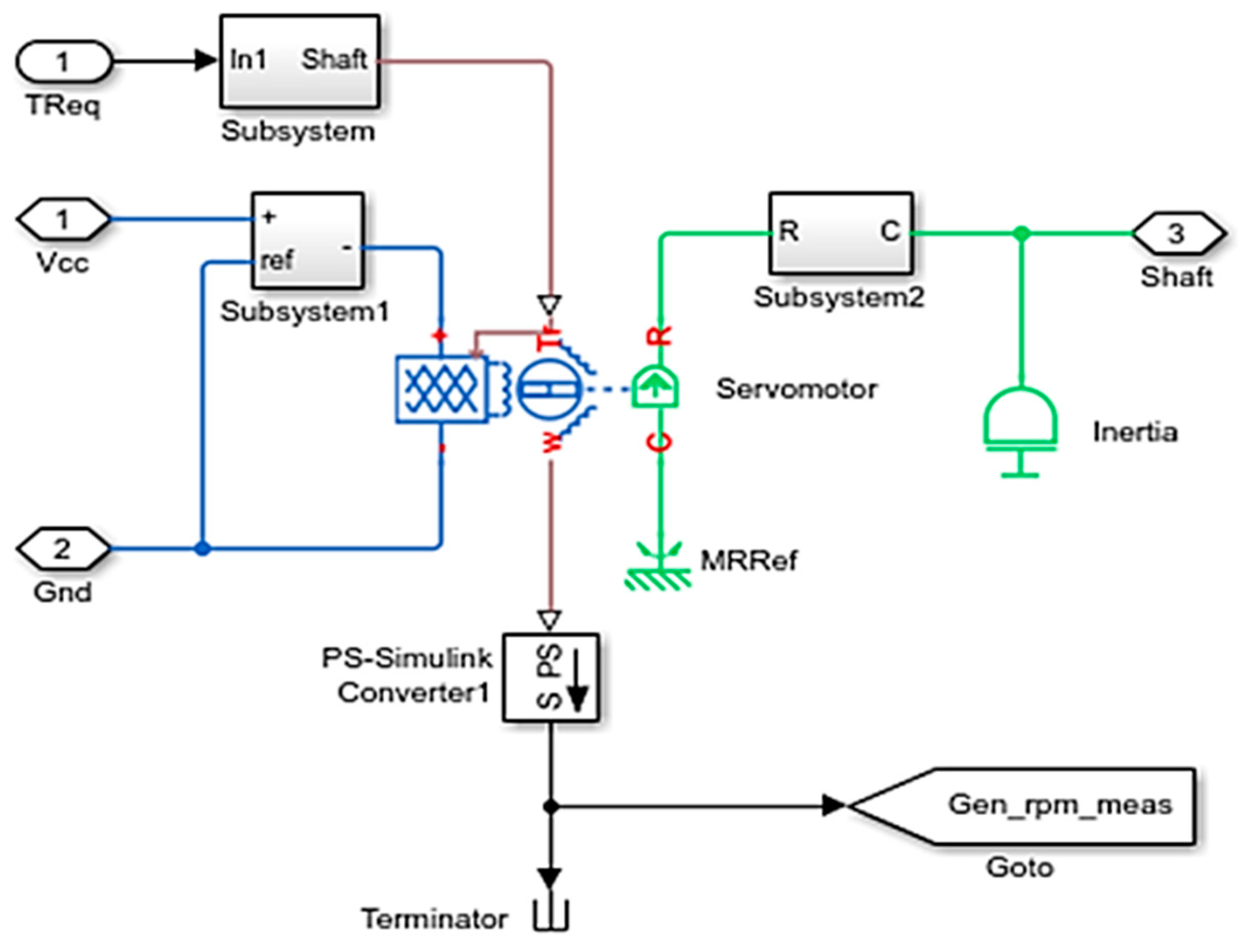
3.3. Model of the Starter/Generator

A typical starter/generator motor is drawn for modelling the generator and motor; the output torque of this motor is achieved from the reference of the torque demand generated at the control centre. Both servo generator and servo motor are supplied from the DC source supplier. The motor is used to provide the necessary torque to the transmission for propelling the HEVs, while the starter/generator motor starts the ICE and charges the vehicle battery via a regenerative braking system regulated from the control centre. Figure 5 and Figure 6 show the model of the generator and motor in Simulink, the blue colour in both figures symbolises the model’s electric parts, and green colour symbolises some mechanical parts.
There are three operation modes for the generator and motor:
Operation at Propulsion:
When the motor is running via this mode, it provides the propulsion torque to the HEVs and the motor operations can be defined by the following:
T o r q u e   o u t p u t :   τ m o t = τ d e m a n d + τ s p i n   l o s s + J m o t d ω d t
T o r q u e   c o n s t r a i n :   τ m o t m a x ( τ m o t ) = f ( ω )
T o r q u e   l o s s i n g   p i n :   τ s p i n   l o s s = α 1 δ ( t ) + α 2 ω + α 3 s g n ( ω )
P o w e r   r e q u i r e d   P e l e c = P m e c h η m o t = τ m o t ω η ( τ m o t , ω )
E f f i c i e n c y :   η m o t = η ( τ m o t , ω )
V o l t a g e :   V m o t = V b u s
C u r r e n t :   I m o t = P e l e c V b u s
where J m o t is the motor inertia, τ m o t is the propulsion torque in Nm, and τ s p i n   l o s s is the friction torque in Nm. Similarly, τ d e m a n d is the demand torque in Nm from the HEVs, ω is the angular speed in rpm, and max ( τ m o t ) equal to f(ω) is the maximum motor torque. α 1 , α 2 , and α 3 are the coefficient static friction, viscous resistance, and Coulomb coefficient, correspondingly; these coefficients can be calculated from the availability of the tested data. η m o t is the lumped efficiency from the inverter, controller, and motor. V b u s is the DC bus volt.
Operation at Regenerative Power:
Once the motor is running at regenerative power, the generator charges the HEV’s battery and the brake torque for the HEVs. During this mode, the generator operation is written as follows:
B r a k e   t o r q u e :   τ a t   r e g e n   e q u a l   t o   τ demand   minus   τ spin   loss + J mot d ω dt
T o r q u e   c o n t r a i n :   τ a t   regen     max ( τ regen ) = g ( ω )
T o r q u e   i n   l o s t   p i n :     τ spin   loss = α 1 + α 2 ω + α 3 sgn ( ω )
P o w e r :   P elect = η regen × P mech   e q u a l   t o   η ( τ regen ,   ω ) × τ regen × ω
E f f i c i e n c y :   η mot = η ( τ regen , ω )
V o l t a g e :   V mot = V bus
C u r r e n t :   I regen = P elec V bus
where J m o t is the motor inertia; τ r e g e n is the torque brake in Nm; and τ d e m a n d is the torque demand from the HEVs in Nm. Additionally, ω is the angular speed in rpm; m a x ( τ r e g e n ) is the maximum regenerative torque; and η m o t is the lumped efficiency regenerative torque of the inverter, generator, and controller.
Operation at Spinning:
When the motor is running at spinning, a slight negative torque friction to the HEVs can be represented as:
τ m o t   e q u a l   t o   τ s p i n t   l o s s = α 1 δ ( t ) + α 2 ω + α 3 s g n ( ω )
where τ m o t is the torque output, and τ s p i n t   l o s s is the torque spinning loss. The coefficients of α 1 , α 2 , and α 3 are the coefficients of the static friction, viscous resistance, and Coulomb coefficient, respectively, on the starter/generator.

3.4. Model of the Planetary Gear

The planetary gear can be used in HEVs for an automated gearbox and for the connection of power splitting. In an automated gearbox of 6 speeds, 3 separated planetary gears are used. In HEVs, the planetary gear or epicyclic gearing train has three outputs/inputs, namely, the sun (S), carrier (C), and ring (R). The fundamental formula for the planetary gear train is:
ω C = 1 2 ( ω S + ω R )
where ω C , ω S , and ω R are the angular velocities of the carrier, sun, and ring.
Planetary gear links can be connected to the ICE, electric main motor, and generator. The mechanical model for the planetary gear in the MATLAB 2021b Simulink is shown in Figure 7.

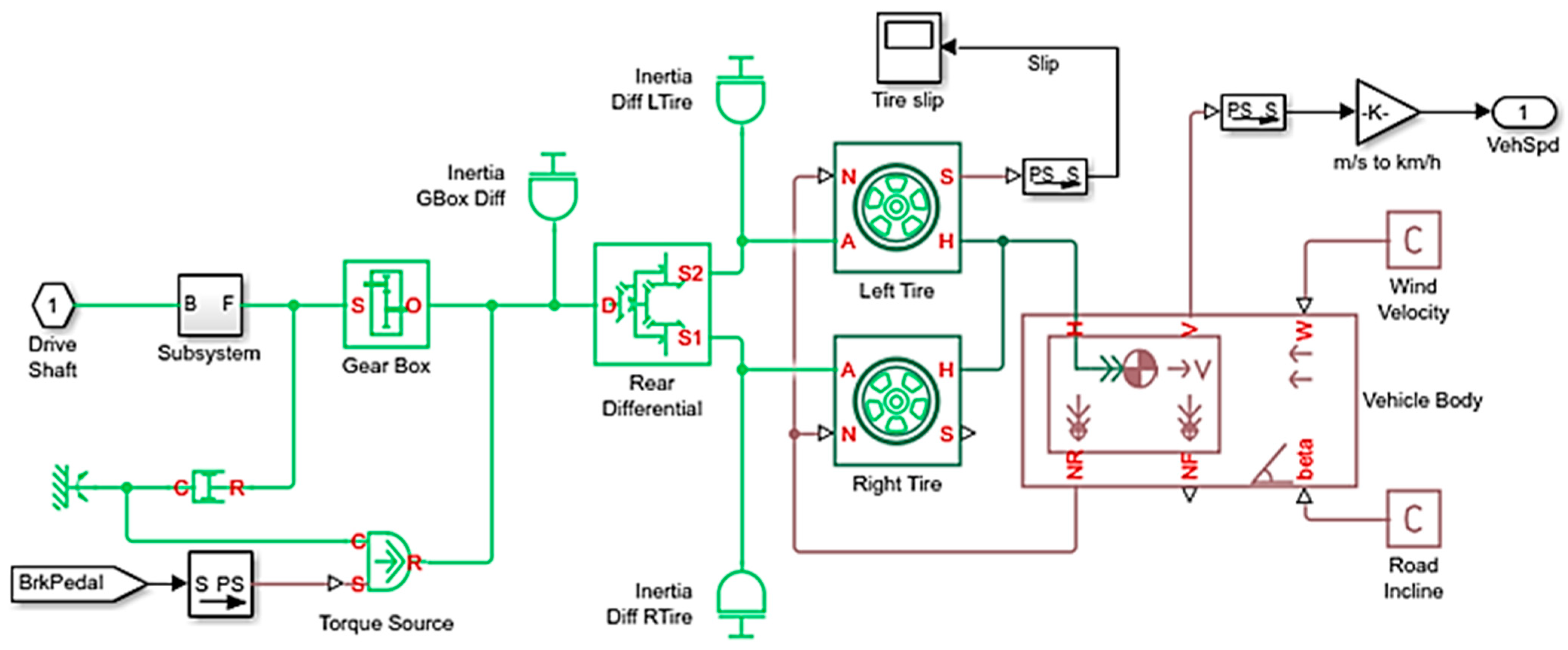
3.5. Model of the Vehicle Dynamics

The model of the vehicle dynamics consists of the torque source, gearbox, differential gear, tires, vehicle body, and road dynamics. The model of the HEV body is shown in Figure 8.
The vehicle body indicates the aero drag and rolling resistance forces. The force of the HEV, when the vehicle is not moving, is calculated as F f r i c + F g r a d e . The force required for propulsion at various speeds is calculated as:
F w h = F r o l l i n g + F a e r o + F g r a d e + m v × a
where F w h is the force traction on the vehicle wheel from the powertrain, m v is the vehicle mass in kg, a is the vehicle acceleration in m/s2, and F r o l l i n g , F a e r o , and F g r a d e are the resistances of the rolling, aero drag, and grade of the weighing forces, correspondingly. These forces are calculated as:
F r o l l i n g     k r r c × k s c × m v × g
F a e r o = k a e r o × v 2
k a e r o = 1 2 × C a × A d × C d × F a
F g r a d e   e q u a l   t o   m v × g × s i n ( α )
where k r r c is the coefficient of the rolling resistance; k s c is the coefficient on the road’s surface; k a e r o is the coefficient of the aero drag; C a is the coefficient of the air density and the change in altitude; A d is the density of the air mass in kg/m3; Cd is the coefficient for the force aerodynamics in N × s 2 k g × m ; F a is the HEV front crossing area in m2; and α is the road angle(up or down) in rad.

3.6. Model of the ICE

The ICE provides the propelling torque, T e n g i n e ( ω e ,   x θ e ) , and the torque from the gearbox, T g , is the load torque on the ICE. The equation for the ICE rotating torque is calculated as:
T e n g i n e ( ω e , x θ e ) T g = I e   d ω e d t
where ω e ,   x θ e and I e are the ICE angular velocity in rpm, the engine throttle or the accelerator pedal position in %, and the equivalent rotating inertia of ICE in kg m2, correspondingly. x θ e is assumed as a position variable ranging from 0% to 100%. The ICE of the HEV is modelled and shown in Figure 9.

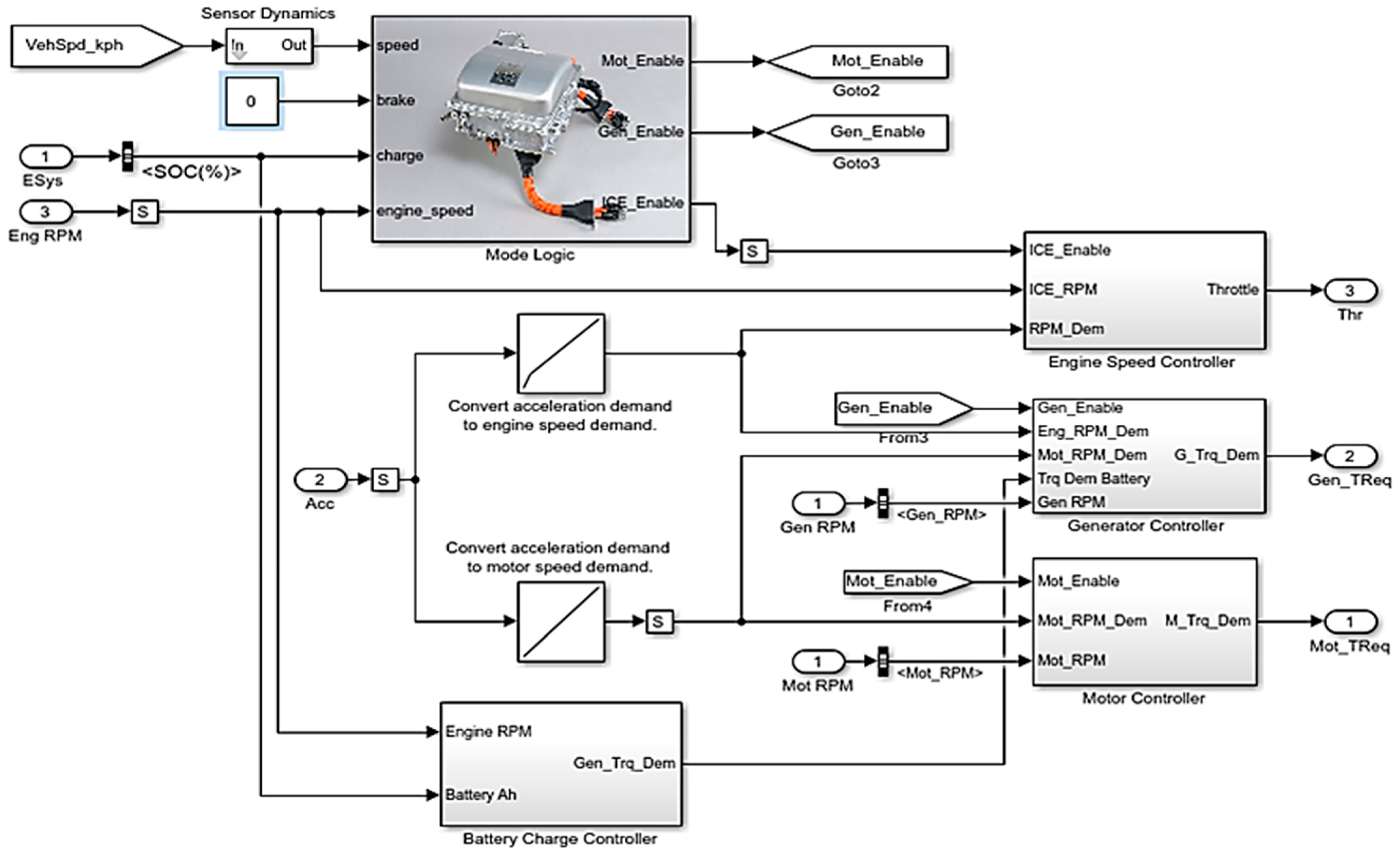
3.7. Model of the Control System

The control centre in an HEV is modelled with several separated sub-blocks, including the motor controller, generator controller, engine speed controller, battery charge controller, and/or converters. The whole control system in Simulink is designed and drawn in Figure 10.

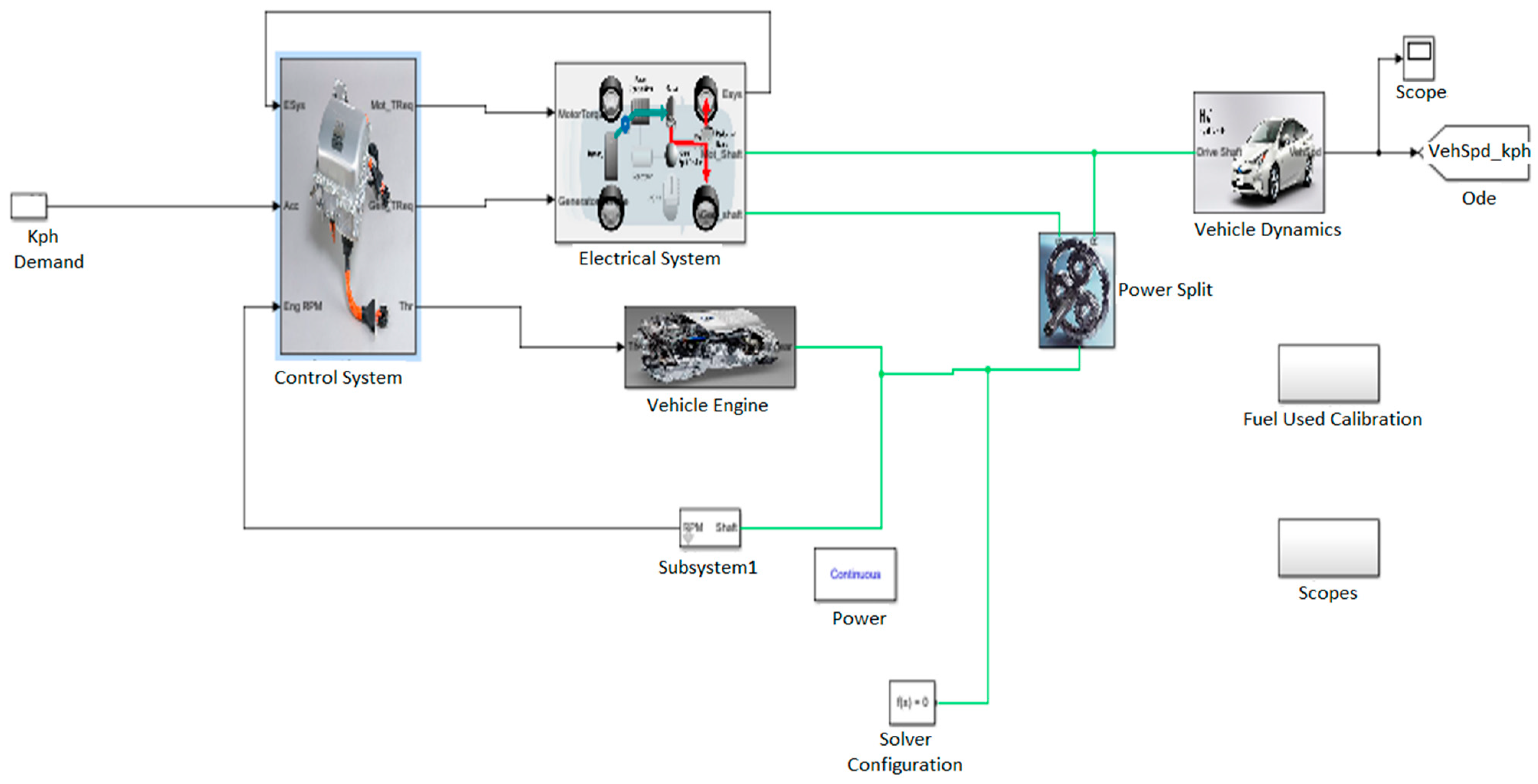
3.8. Model of the Integrated HEV

Finally, the whole integrated HEV model is designed and drawn in Figure 11. The model consists of ICE, motors, control system, electrical system, converters, battery, power split, vehicle dynamics, fuel consumption estimator, and mechanical system.

4. Fuel Economy Modelling and Regressions

The comprehensive HEV model in Simulink in Figure 11 and other Simulink schemes are tested on different HEV models, shown in Table 1, and at the link references [28,29,30,31,32,33,34,35]. Different HEV models are simulated with different tires running on FTP75 (standard urban driving cycles). These 8 HEV models with different weights and different tires, and with 90% fuel in the tank, are run for 100 s on FTP75.
Ten different compatible tire sizes are selected and simulated with the above eight HEV models. These ten different compatible tire parameters are indicated in Table 2.
The calculated fuel consumption values from the above HEV simulations running for 100 s on FEP75 are recorded and displayed at Table 3.
Data for the fuel consumption in Table 3 are processed in MATLAB 2021b to attain the different fuel consumption regression models for HEVs based on their weights and tires. The fuel consumption is a function of the above data and depending on the function order:
C o n s u m p t i o n   o f   F u e l   F = f u n c t i o n   ( H E V s   w e i g h t   W ,   a n d   r a d i u s   T i r e s   T )
Now, we consider the first-order fuel regression model in the following form:
F 1 = f 1 ( W , T ) = P 00 + P 10 W + P 01 T
where F1 is the first-order regression model for the fuel consumption, W is the HEV’s Weight, T is the Tire radius, and the coefficients of P 00 , P 10 , and P 01 are generated as P00 = 0.02015; P10 = 0.0006672; and P01 = 0.0002534, correspondingly. The first-order fuel regression model from (42) has the determination coefficient of R-square = 0.5364, or this regression prediction fits the data of 53.64%.
Next, we consider the second-order fuel regression model in the following form:
F 2 = f 2 ( W , T ) = P 00 + P 10 W + P 01 T + P 20 W 2 + P 11 W T + P 02 T 2
where F2 is the consumption of fuel in the second-order regression model; W is the HEV’s Weight, T is the Tire radius, and the coefficient of P 00 , P 10 , P 01 , P 20 , P 11 , and P 02 are generated as P 00 = 0.01946; P 10 = 0.0004894; P 01 = 0.0002958; P 20 = 0.0005422; P 11 = 0.0004614; and P 02 = 0.0001364, correspondingly. The second-order regression equation model in (43) has the determination coefficient of R-square = 0.8875, or this regression prediction fits the data of 88.75%.
Finally, we consider the third-order fuel regression model in the following form:
F 3 = f 3   ( W , T ) = P 00 + P 10 W + P 01 T + P 20 W 2 + P 11 W T + P 02 T 2 + P 30 W 3 + P 21 W 2 T + P 12 W T 2 + P 03 T 3
where F 3 is the consumption of fuel in the third regression model; W is the HEV’s Weight, T is the Tire radius, and the coefficients of P 00 , P 10 , P 01 , P 20 , P 11 , P 02 , P 30 , P 21 , P 12 , and P 03 are generated as P 00 = 0.01948; P 10 = −8.057 × 10⁻⁵; P 01 = −8.597 × 10⁻⁵; P 20 = 0.0004235; P 11 = 0.0004004; P 02 = 0.0001391; P 30 = 0.0003122; P 21 = 0.0003401; P 12 = 0.000162; and P 03 = 2.06 × 10⁻⁵. The third-order regression equation model in (44) has the determination coefficient of R-square = 0.9914, or this regression prediction fits the data of 99.14%.
The 3D graphic map of this HEV’s fuel consumption is drawn out in x, y, z coordinates, where the z-axis is the fuel consumption in litres, the x-axis is the HEV weights in kg, and the y-axis is the tire radius in meters. The range of fuel consumption is from 0.02 to 0.025 litres for the HEVs running for 100 s surrounding the standard driving urban cycle of FEP75. Details of this equation in a 3D graphic map for the fuel consumption vs. HEV weights vs. tires are shown in Figure 12.
The minimum values of the HEV performances on the 3D graphic map and from the third-order regression model in (44) can be attained. When we obtain the first derivative of (44), we can find out the local maximum and the local minimum values of this function. When we continue to obtain the second derivative of this function and if the second derivative function results in f″(W, T) > 0, then the original function, f(W, T), has the local minimum values fmin at Wmin and Tmin.
Taking the derivative Function (44) for F 3 = f 3 ( W , T ) , leads to the optimal values of T and W:
3.0541 × 10 6 · W + 0.0211 · T 0.0095 = 0
Equation (45) permits the achievement of the optimal values of HEVs for fuel consumption from specified weights and tires. The optimal HEV weights by the tires are indicated in Table 4.
Finally, the optimal fuel consumption in (44) and (45) is tested and compared to similar HEVs to observe the efficiency of the optimal HEV’s fuel consumption performances during the different standard driving cycles of EUDC, HWFET, NYCC, and FTP75. In this test, we selected the optimal HEV weight of 1222 kg vs. the rolling tire radius of 0.278 m from the right-hand side column in Table 4. We compared the optimal HEVs to the standard lighter HEVs with a weight of 1200 kg and with a smaller tire radius of 0.262 m. The results for the fuel consumption for optimal HEVs vs. normal HEVs during different driving cycles are shown in Table 5.
Table 5 proves that fuel consumption for optimal HEV models is always less than the similar normal HEV performances with lighter weights and smaller tire radiuses. The results of the simulation re-affirmed that the optimal HEV data in Equation (44) and in the 3D graphic map in Figure 12 are the correct regressions.

5. Conclusions

This study reviewed the latest developments of fuel consumption economy for HEV configurations, controls, and energy managements. Then, the study presented the typical and fundamental HEV modelling and simulation schemes. The final HEV Simulink models were tested on different driving cycles with different HEV weights and tire radiuses. The data obtained from these simulations ere used to set up different regression fuel models. Then, the best-fit regression model was obtained with the determination coefficient R-square of more than 99%, or this regression fuel model represents more than 99%, thus fitting the data perfectly. Finally, the optimal HEVs were tested and compared with the normal HEVs to reconfirm the improvement of the optimal HEVs regarding fuel consumption for different standard driving cycles.

Author Contributions

Conceptualization, V.T.M.; methodology, V.T.M.; formal analysis, V.T.M.; writing—original draft preparation, V.T.M. and R.M.; writing—review and editing, V.T.M., R.M. and J.C.; final edition and supervision, V.T.M. and J.H. All authors have read and agreed to the published version of the manuscript.

Funding

The result was obtained through financial support from the Ministry of Education, Youth and Sports in Czechia and the European Union in the framework of the project “Modular platform for autonomous chassis of specialized electric vehicles for freight and equipment transportation”, Reg. No. CZ.02.1.01/0.0/0.0/16_025/0007293.

Informed Consent Statement

Informed consent was obtained from all subjects involved in the study. Participants were informed that their responses to the questionnaire would be treated entirely anonymously and confidentially.

Data Availability Statement

The data are available from the corresponding author upon request.

Conflicts of Interest

The authors declare no conflict of interest.

References

  1. Ehsani, M.; Singh, K.V.; Bansal, H.O.; Tafazzoli, R. State of the Art and Trends in Electric and Hybrid Electric Vehicles Proc. IEEE 2021, 109, 967–984. [Google Scholar] [CrossRef]
  2. Puma-Benavides, D.S.; Izquierdo-Reyes, J.; Calderon-Najera, J.d.D.; Ramirez-Mendoza, R.A. A Systematic Review of Technologies, Control Methods, and Optimization for Extended-Range Electric Vehicles. Appl. Sci. 2021, 11, 7095. [Google Scholar] [CrossRef]
  3. Faris, W.F.; Rakha, H.A.; Kafafy, R.I.; Idres, M.; Elmoselhy, S. Vehicle fuel consumption and emission modelling: An in-depth literature review. Int. J. Veh. Syst. Model. Test. 2011, 6, 318–395. [Google Scholar] [CrossRef]
  4. Tamada, S.; Bhattacharjee, D.; Dan, P.K. Review on automatic transmission control in electric and non-electric automotive powertrain. Int. J. Veh. Perform. 2020, 6, 98–128. [Google Scholar] [CrossRef]
  5. Singh, K.V.; Bansal, H.O.; Singh, D. A comprehensive review on hybrid electric vehicles: Architectures and components. J. Mod. Transp. 2019, 27, 77–107. [Google Scholar] [CrossRef] [Green Version]
  6. Yang, C.; Zha, M.; Wang, W.; Liu, K.; Xiang, C. Efficient energy management strategy for hybrid electric vehicles/plug-in hybrid electric vehicles: Review and recent advances under intelligent transportation system. IET Intell. Transp. Syst. 2020, 14, 702–711. [Google Scholar] [CrossRef]
  7. Tung, S.C.; Woydt, M.; Shah, R. Global Insights on Future Trends of Hybrid/EV Driveline Lubrication and Thermal Management. Front. Mech. Eng. 2020, 6, 571786. [Google Scholar] [CrossRef]
  8. Jiang, J.; Jiang, Q.; Chen, J.; Zhou, X.; Zhu, S.; Chen, T. Advanced Power Management and Control for Hybrid Electric Vehicles: A Survey. Wirel. Commun. Mob. Comput. 2021, 2021, 6652038. [Google Scholar] [CrossRef]
  9. Meng, Z.; Tang, G.; Zhou, Q.; Liu, B. A Review of Hybrid Electric Vehicle Energy Management Strategy Based on Road Condition Information. In Proceedings of the IOP Conference Series: Earth and Environmental Science, Surakarta, Indonesia, 24–25 August 2021. [Google Scholar]
  10. Zhang, F.; Hu, X.; Langari, R.; Cao, D. Energy management strategies of connected HEVs and PHEVs: Recent progress and outlook. Prog. Energy Combust. Sci. 2019, 73, 235–256. [Google Scholar] [CrossRef]
  11. Shi, T.; Zhao, F.; Hao, H.; Liu, Z. Development Trends of Transmissions for Hybrid Electric Vehicles Using an Optimized Energy Management Strategy. Automot. Innov. 2018, 1, 291–299. [Google Scholar] [CrossRef] [Green Version]
  12. Galvagno, E.; Guercioni, G.; Rizzoni, G.; Velardocchia, M.; Vigliani, A. Effect of Engine Start and Clutch Slip Losses on the Energy Management Problem of a Hybrid DCT Powertrain. Int. J. Automot. Technol. 2020, 21, 953–969. [Google Scholar] [CrossRef]
  13. Zou, Y.; Huang, R.; Wu, X.; Zhang, B.; Zhang, Q.; Wang, N.; Qin, T. Modeling and energy management strategy research of a power-split hybrid electric vehicle. Adv. Mech. Eng. 2020, 12, 12. [Google Scholar] [CrossRef]
  14. Heppeler, G.; Sonntag, M.; Sawodny, O. Fuel efficiency analysis for simultaneous optimization of the velocity trajectory and the energy management in hybrid electric vehicles. IFAC Proc. Vol. 2014, 47, 6612–6617. [Google Scholar] [CrossRef] [Green Version]
  15. Xu, Q.; Wang, F.; Zhang, X.; Cui, S. Research on the Efficiency Optimization Control of the Regenerative Braking System of Hybrid Electrical Vehicle Based on Electrical Variable Transmission. IEEE Access 2019, 7, 116823–116834. [Google Scholar] [CrossRef]
  16. Reksowardojo, I.K.; Arya, R.R.; Budiman, B.A.; Islameka, M.; Santosa, S.P.; Sambegoro, P.L.; Aziz, A.R.A.; Abidin, E.Z.Z. Energy management system design for good delivery electric trike equipped with different powertrain configurations. World Electr. Veh. J. 2020, 11, 76. [Google Scholar] [CrossRef]
  17. Yao, Z.; Yoon, H. Control Strategy for Hybrid Electric Vehicle Based on Online Driving Pattern Classification. SAE Int. J. Altern. Powertrains 2019, 8, 8. [Google Scholar] [CrossRef]
  18. Sim, K.; Oh, S.; Namkoong, C.; Lee, J.; Han, K.; Hwang, S. Control strategy for clutch engagement during mode change of plug-in hybrid electric vehicle. Int. J. Automot. Technol. 2017, 18, 901–909. [Google Scholar] [CrossRef]
  19. Wang, S.; Xia, B.; He, C.; Zhang, S.; Shi, D. Mode transition control for single-shaft parallel hybrid electric vehicle using model predictive control approach. Adv. Mech. Eng. 2018, 10, 10. [Google Scholar] [CrossRef] [Green Version]
  20. Robuschi, N.; Zeile, C.; Sager, S.; Braghin, F. Multiphase mixed-integer nonlinear optimal control of hybrid electric vehicles. Automatica 2021, 123, 109325. [Google Scholar] [CrossRef]
  21. Wróblewski, P.; Kupiec, J.; Drozdz, W.; Lewicki, W.; Jaworski, J. The Economic Aspect of Using Different Plug-In Hybrid Driving Techniques in Urban Conditions. Energies 2021, 14, 3543. [Google Scholar] [CrossRef]
  22. Mahroogi, F.O.; Narayan, S. A recent review of hybrid automotive systems in Gulf Corporation Council region. Proc. Inst. Mech. Eng. Part D J. Automob. Eng. 2019, 233, 3579–3587. [Google Scholar] [CrossRef]
  23. Miri, I.; Fotouhi, A.; Ewin, N. Electric vehicle energy consumption modelling and estimation-A case study. Int. J. Energy Res. 2021, 45, 501–520. [Google Scholar] [CrossRef]
  24. Heni, H.; Arona Diop, S.; Renaud, J.; Coelho, L.C. Measuring fuel consumption in vehicle routing: New estimation models using supervised learning. Int. J. Prod. Res. 2021, 1–17. [Google Scholar] [CrossRef]
  25. Minh, V.T. Advanced Vehicle Dynamics; Universiti of Malaya Press: Kuala, Lumpur, 2012; Volume 265. [Google Scholar]
  26. Minh, V.T.; Mohd Hashim, F. Adaptive teleoperation system with neural network-based multiple model control. Math. Probl. Eng. 2010, 2010, 592054. [Google Scholar] [CrossRef] [Green Version]
  27. Minh, V.T.; Afzulpurkar, N. Robustness of model predictive control for Ill-conditioned distillation process. Dev. Chem. Eng. Min. Process. 2005, 13, 311–316. [Google Scholar] [CrossRef]
  28. Hybrid Toyota Prius. 2021. Available online: https://www.toyota.com/prius (accessed on 4 October 2021).
  29. Hybrid Honda Insight. 2021. Available online: https://automobiles.honda.com/insight (accessed on 4 October 2021).
  30. Hybrid Kia Niro. 2021. Available online: https://www.kia.com/cz/modely/niro/objevte (accessed on 4 October 2021).
  31. Hyundai Sonata. 2021. Available online: https://www.hyundaiusa.com/us/en/vehicles/sonata-hybrid (accessed on 4 October 2021).
  32. Hybrid Kia Optima. 2021. Available online: https://www.kia.ca/vehicles/optimahybrid/overview (accessed on 4 October 2021).
  33. Hybrid Hyundai Avante LPi. 2021. Available online: https://www.hyundai.com/worldwide/en/ (accessed on 4 October 2021).
  34. Hybrid Toyota Camry. 2021. Available online: https://www.toyota.com/camryhybrid/ (accessed on 4 October 2021).
  35. Hybrid Honda Civic. 2021. Available online: https://automobiles.honda.com/civic (accessed on 4 October 2021).
  36. Minh, V.T.; Moezzi, R.; Cyrus, J.; Dhoska, K. Smart Mechatronic Elbow Brace using EMG Sensors. Int. J. Innov. Technol. Interdiscip. Sci. 2022, 5, 865–873. [Google Scholar]
  37. Minh, V.T.; Katushin, N.; Moezzi, R.; Dhoska, K.; Pumwa, J. Smart Glove for Augmented and Virtual Reality. Int. J. Innov. Technol. Interdiscip. Sci. 2021, 4, 663–671. [Google Scholar] [CrossRef]
  38. Minh, V.T.; Moezzi, R.; Dhoska, K.; Pumwa, J. Model Predictive Control for Autonomous Vehicle Tracking. Int. J. Innov. Technol. Interdiscip. Sci. 2021, 4, 560–603. [Google Scholar]
  39. Minh, V.T.; Tamre, M.; Musalimov, V.; Kovalenko, P.; Rubinshtein, I.; Ovchinnikov, I.; Moezzi, R. Simulation of Human Gait Movements. Int. J. Innov. Technol. Interdiscip. Sci. 2020, 3, 326–345. [Google Scholar]
Figure 1. HEV parallel powertrain scheme.
Asi 05 00036 g001
Figure 2. Modelling HEV’s powertrain.
Asi 05 00036 g002
Figure 3. Battery model.
Asi 05 00036 g003
Figure 4. DC to DC converter.
Asi 05 00036 g004
Figure 5. Starter model.
Asi 05 00036 g005
Figure 6. Generator model.
Asi 05 00036 g006
Figure 7. Planetary gear train.
Asi 05 00036 g007
Figure 8. Model of HEV body.
Asi 05 00036 g008
Figure 9. ICE model in Simulink.
Asi 05 00036 g009
Figure 10. Modelling control system.
Asi 05 00036 g010
Figure 11. Simulink model for the HEV.
Asi 05 00036 g011
Figure 12. The best-fit fuel consumption model, 99.14%.
Asi 05 00036 g012
Table 1. HEV weights.
No.HEV ModelsHEV Weights in Kg
1.Hybrid Toyota Prius 2021 1335 [28]
2.Hybrid Honda Insight 20211247 [29]
3.Hybrid Kia Niro 20211419 [30]
4.Hyundai Sonata 20211578 [31]
5.Hybrid Kia Optima 20211595 [32]
6.Hybrid Hyundai Avante LPi 20211287 [33]
7.Hybrid Toyota Camry 20211639 [34]
8.Hybrid Honda Civic 20211270 [35]
Table 2. Ten different tires for HEVs.
No.ParametersRolling Radius in MetersRim Width in Inch
1.154/65/R130.2424.5
2.154/80/R130.2624.5
3.164/60/R140.2525.0
4.164/65/R130.2465.0
5.164/65/R140.2575.0
6.164/70/R140.2675.0
7.164/80/R130.2684.5
8.174/65/R140.2655.0
9.174/65/R150.2755.0
10.204/50/R150.2766.5
Table 3. Fuel consumption in litre.
13351247141915781595128716391270
0.2420.019830.019830.019840.019920.019940.019830.020080.01983
0.2620.019620.019620.019650.020330.020530.019620.021820.01962
0.2520.019720.019720.019720.01980.019940.019720.020520.01972
0.2460.019780.019780.019780.019920.019940.019980.020250.01978
0.2570.019670.019650.019690.019960.020260.019650.021220.01965
0.2670.019550.019560.019560.020560.020870.019560.022540.01956
0.2680.019540.019550.019580.020920.021280.019520.023230.01955
0.2650.019570.019580.019610.020440.020620.019570.022080.01957
0.2750.019470.019470.019550.021870.022370.019460.025120.01946
0.2760.019610.019610.019640.020240.020450.019610.02150.01961
Table 4. Optimal HEV weights vs. tire radiuses.
Rolling Tire Radius in Meters0.2420.2480.2520.2590.2620.2650.2670.2690.2770.278
Optimal HEV Weights in Kg1472142914021354133313121298127712291222
Table 5. Compared fuel consumption of optimal vs. normal HEVs.
NoHEV TypeDriving CycleHEV Weight in KgTire Radius in MetersFuel Consumption in Litres
1.Normal
Optimal
FTP751200
1222
0.262
0.278
0.03667
0.03648
2.Normal
Optimal
NYCC1200
1222
0.262
0.278
0.03294
0.03262
3.Normal
Optimal
HWFET1200
1222
0.262
0.278
0.03968
0.03914
4.Normal
Optimal
EUDC1200
1222
0.262
0.278
0.03714
0.03654
Publisher’s Note: MDPI stays neutral with regard to jurisdictional claims in published maps and institutional affiliations.

