2. Methodology
To evaluate the impact of different PEV penetration rates and PV sizing on a microgrid over an investment period, a sport center microgrid is examined. The case study employed for this paper is the Olympic Athletic Center of Athens (OAKA). Part of the data which naturally follows a stochastic behavior, i.e., the PEV arrivals/departures, etc., was created to represent the state of the real world as best as possible. The energy price that is bought and sold to the grid is considered to have the same electricity price. Finally, no wind turbines were considered because of their size and unsuitability to the examined area (urban site).
2.1. PEV and Charger Type
The initial considerations have to do with the PEV and Charger types. It was assumed that the percentage of PEVs that would charge at the microgrid would consist of 75% passenger EVs, 15% electric two wheelers (ETW) and 10% electric buses (EB). PEV appearance possibility is equal to its related market share. [
17]. Their technical characteristics and charging limitations are shown in
Table 1. The values for the charging limitation that were not known appear in
Table 1 with the sign “*”and a value which is considered suitable is assigned to them [
18].
In addition, it is considered that all PEVs support bidirectional energy flow and the charging and discharging have the same power limitations. Two types of chargers are considered, an alternative current (AC) of 22 kW and a direct current (DC) of 100 kW.
2.2. PEV Arrival, Departure and State of Charge
It is considered that the drivers that charge their PEV at OAKA are the drivers that work and exercise in the sport center, the drivers living in the nearby area as well as the drivers who charge their PEV at OAKA as a stopover before their destination. Most people go to work between 7:00 to 9:00. Furthermore, the majority of sport activities are between 9:00 to 13:00 and 17:00 to 20:00. Hence, most of the arrivals are estimated to take place in these hours as the majority of the PEV drivers who parked at the sport center are those who are training there. Moreover, most people return from their morning work between 15:00 to 17:00. Taking the above into consideration, the arrival profile of PEV is presented in
Figure 1. Number of PEVs represent the number of PEV that charge at the sport center every day. Five different scenarios are considered as explained in
Section 4.
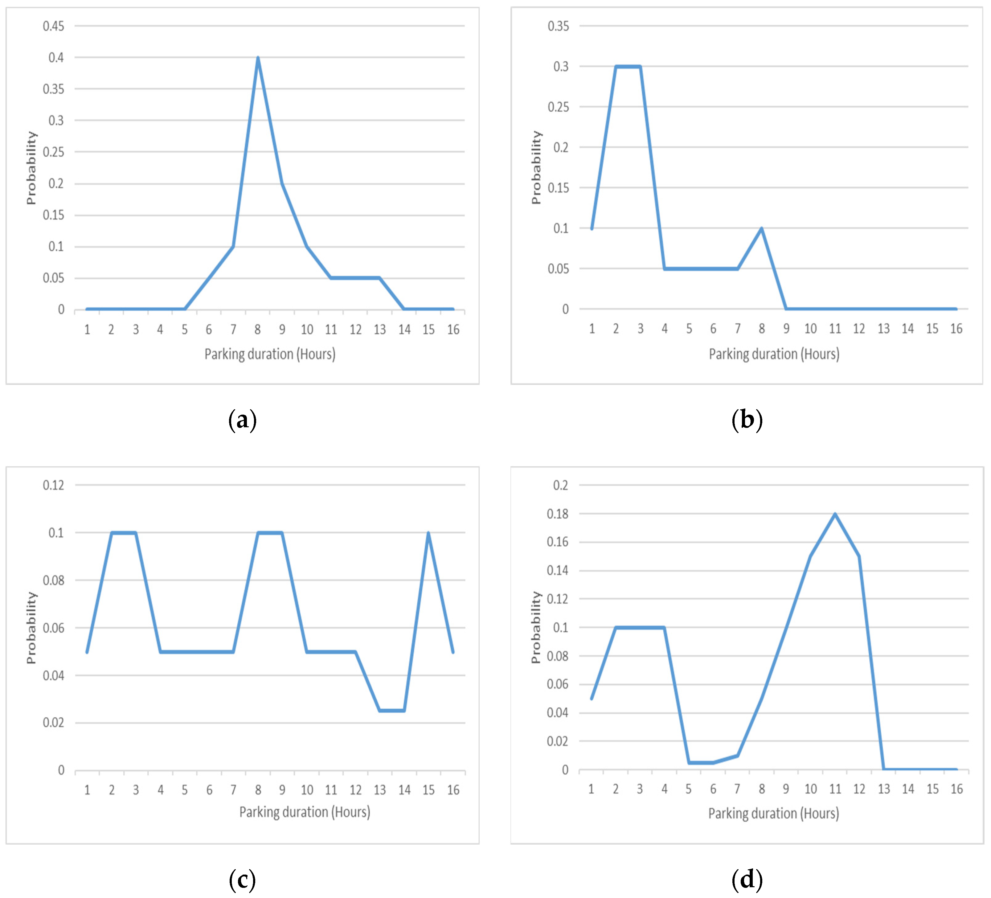
The duration of sport activities is usually between 1 to 4 h. In addition, most people work about 8 to 9 h. Hence, the parking duration probability depending on the arriving time is presented in
Figure 2.
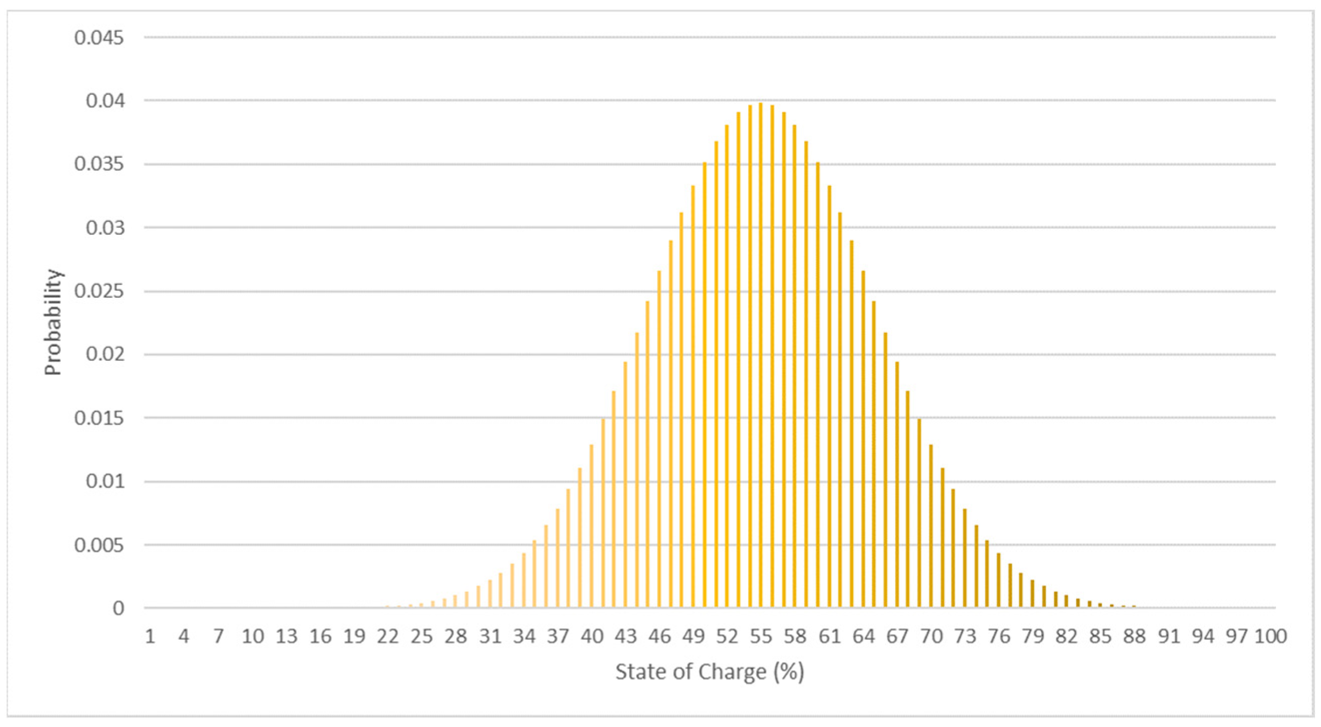
The probability arriving SoC of the PEVs was estimated as in [
1].
Figure 3 depicts the probability of the arriving PEV’s SoC.
2.3. PEV Charging Scheduling
In this section the two charging strategies of the case study will be discussed. In particular, the first strategy corresponds to uncoordinated charging strategy while the second is the one proposed in this paper.
2.3.1. Uncoordinated Charging Strategy
Uncoordinated charging is the process that the charging of the PEV starts when the PEV plugs into the charger with its nominal power until the PEV’s departure SoC is satisfied [
18].
2.3.2. Proposed Charging Strategy
A rule-based algorithm is used in order to schedule the PEV charging. At first, the charging is assigned to the time slots with the lowest electricity price. The time slot is considered as a time period of Δt = 1 h. Then, a search takes place to find if there are time slots that the PEV can discharge and recharge in a profitable manner. More particular, it searches the time slots with the lowest (t
1) and the highest (t
2) electricity price during the parking session in which the charging power is under the permitted power limit, as it is explained below in the charging constrains. The condition that must apply in order for the PEV to participate in the discharging process is shown in Equation (1). Finally, the discharging power is calculated depending on the available charging power at the t
1 and t
2.
where n
ch and n
dis are the charging and discharging efficiencies. In this study they are considered equal, and both are being represented by the n parameter. This coefficient is considered to be equal to 0.93 and it represents the energy losses during the charging and discharging process. The t
B and t
S are the time slots that the energy will be bought from and sold to the grid, respectively. C is the electricity price. The flowchart of the proposed charging strategy is illustrated in
Figure 4.
The charging constrains are formulated in Equations (2)–(4).
where P
limit depends on the charger and PEV power limitation, E
min(i) is the lowest energy limit of the ith PEV which is considered the 20% of the SoC and E
max(i) is the upper power limit which is considered 100% of the SoC. The ch(i,t) is a binary variable set to 1 when the P(i,t) is positive and 0 otherwise. Similarly for the dch(i,t), with the differentiation that it is set to 1 when P(i,t) is negative. E
D(i) is the desirable energy of the ith PEV during its departure.
In fact, the algorithm calculates the PEV charging schedule based solely on the electricity price criterion. Hence, in this format, the discussed charging strategy would not take into consideration the PV production. The proposed charging method that is taking into consideration only the electricity pricy is referred as s1. A modification in the price, that the proposed algorithm is taking as criterion, is introduced as shown in Equation (5) to alleviate this issue. This case of the proposed charging method is referred to as s2. The charging cost in the case of the s2 is evaluated with the real electricity price.
Seasonal average PV generation curves are estimated from the known yearly data of the PV generation in order to calculate the factor c1 which varies between 0 and 1. When the estimated PV generation is the lowest, then c1 is set to 0 and vice versa. c2 is a value that is set between 0 and 1 depending on the electricity price during the parking period of each PEV. It is set to 1 when the electricity price gets its maximum value during the parking duration and to 0 when the electricity price gets its minimum value. In particular, in s1, during the parking duration, energy is saved to the PEVs’ battery when the electricity price is relatively “low”. The energy is sold back to the grid or supplies the microgrid when the electricity price is relatively “high”. In s2, PEVs store energy from RES and the grid when the electricity price is relatively “low”, and sell it back to the grid when the electricity price is relatively “high” or supply the microgrid.
2.4. Microgrid Power Balance
It is considered that the microgrid will consist of PV, PEV chargers and the loads from the sport facilities. It will also be connected to the grid. The power balance is presented in the equation below:
where the energy consumption and supply are represented by the left-handed and right-handed side, respectively. P
L is the load from the sport facilities, P
Ch is the load from PEV charging and P
SG is the power sold to the grid. On the other side, P
PV is the energy generated from the PVs, P
Dch is the energy from the PEV discharging and P
BG is the power bought to the grid.
The dispatched power from PVs depends mainly on the installed capacity and the weather conditions.
2.5. Financial Model
In order to evaluate the investment financially, a discount cash flow method is applied. The net present value (NPV) is a method used to determine if an investment is profitable, by calculating the future cash inflow and outflow over the investment lifetime, discounted to the present. NPV is calculated in Equation (7).
where R
y is the net cash flow during the year y, i is the discount rate and N is the investment lifetime. Ins
Cost and O&E
Cost are the installation, and operation and maintenance costs, respectively. S&R are the savings and revenues due to the investment. The savings are the difference of the electrical cost with and without the PVs. The revenues are calculated from the energy sold to the grid from the PV and PEV discharging if V2G is considered. The investment period is set to 25 years, similar to the lifetime of the PV. S&R and O&E
Cost are set to 0 when y = 0 and Int
Cost is set to 0 when y ≠ 0. The year y = 0 is the year that the investment takes place.
In the case study, primarily, the NPV is calculated for the uncoordinated charging strategy. Then, a comparison between the cash flow of uncoordinated and proposed charging strategy is done considering PV generation and the investment period, and it is discounted to the present. This process estimates the contribution of the proposed charging strategy (s1 and s2) versus the uncoordinated strategy expressed in monetary value.
2.6. Extrapolation Monthly Results to One Year
The PV generation and the load of a generic microgrid vary during the year but they have similar behavior during the months of the same season. To calculate the economic effect of the PV sizing and the PEV penetration rate on a microgrid it is important to examine at least one year, in order to obtain statistically strong results. In order to reduce the extensive computations of the one-year calculations, and building on the fact that the PV generation and the load of the microgrid are similar between the months of the same season, four representative months are considered in this study, one for each season. The results of each selected month are multiplied by 3 in order to extrapolate the results to those of one year. In this way, the computation time and the accuracy of the results can balance out, as it was also pointed out in [
8]. The months that were selected are March (for spring), June (for summer), September (for autumn) and December (for winter).
3. Case Study
OAKA is supplied by three (3) high/medium voltage (HV/MV) substations (D1, D2 and D3) and there are twenty-two (22) medium/low voltage MV/LV substations. The power limits of the HV/MV substations are
= 6 MVA,
= 8 MVA and
= 6 MVA. The simplified sketch of the considered microgrid is depicted in
Figure 5.
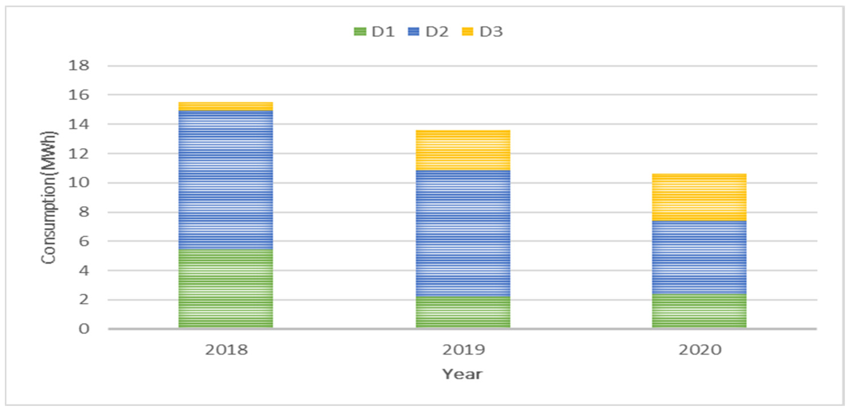
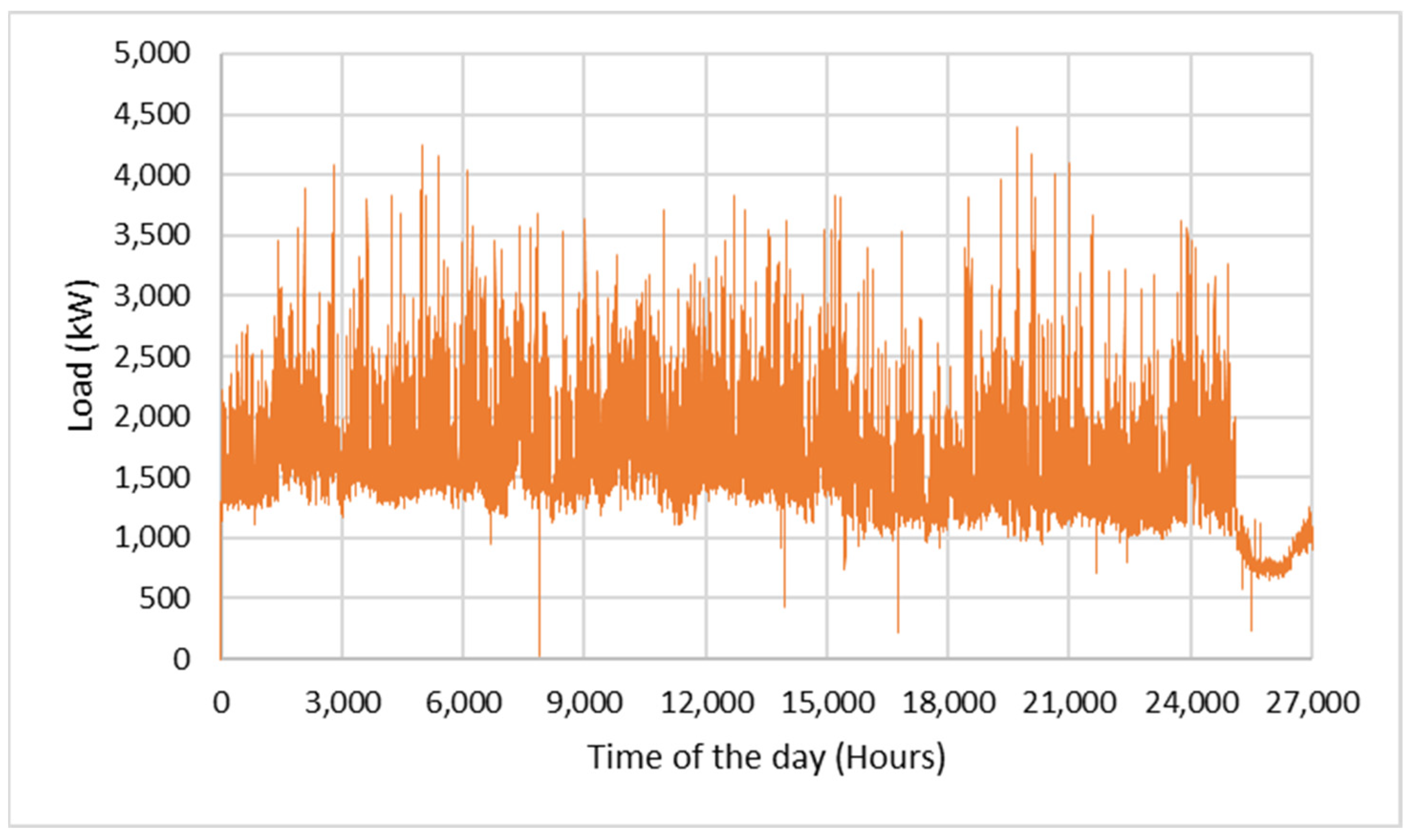
To select the appropriate data for the calculations of the next section, the sport center’s load for the years 2018–2020, is analyzed. Even though the load of the year 2020 was significantly low because of the regulations that were taken during COVID-19 pandemic, the demand peak was higher than the other two years. The total load, the average seasonal load and the load time series of OAKA for the years 2018–2020 are depicted in
Figure 6,
Figure 7 and
Figure 8. Year 2020 was not considered in the calculations because of its extended deviations due to the pandemic. Hence, the load of the OAKA microgrid in the first year of the investment period was estimated as the average demand of the year 2018 and 2019. To incorporate the stochastic behaviour of the consumption of the microgrid, a raise of 1% of the consumption of the initial year for every next year is added, and a random value between −20 and 20 kW is added, too.
According to the power limits of D1, D2 and D3 and the predicted peak power at the end of the investment period, the maximum number of PEV chargers is calculated. The proportion of AC and DC charger was considered 80% and 20%, respectively. The majority of the PEV drivers that use DC chargers are those whose do not have adequate time to charge their PEV at an AC charger in order to reach their next charging point. In addition, most people stay long enough at the sport center and the AC chargers could cover the charging needs. Furthermore, the DC chargers are more expensive. Hence, a small number of PEVs would use DC charger. The maximum number of PEV chargers is 308 AC chargers and 77 DC chargers. In case a PEV arrives, and all chargers are occupied, it will not charge.
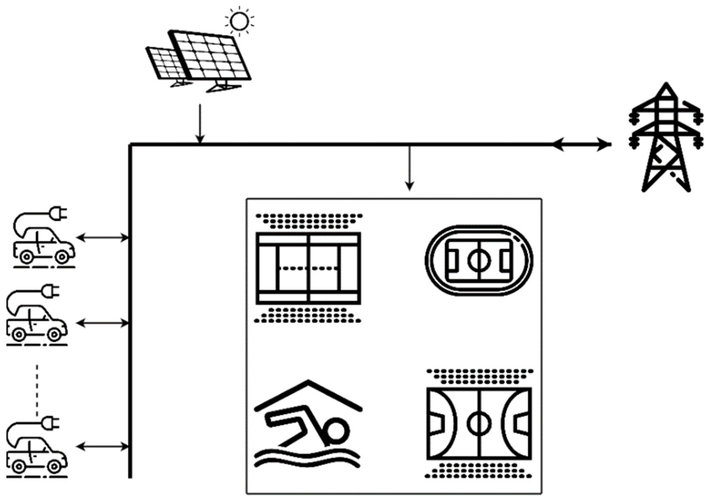
Finally, for simplification purposes the sport center is considered as one unit as illustrated in
Figure 9. The arrows show the energy flow direction. The optimal PV and PEV charger distribution among the H/V substations is not considered in this study.
4. Results
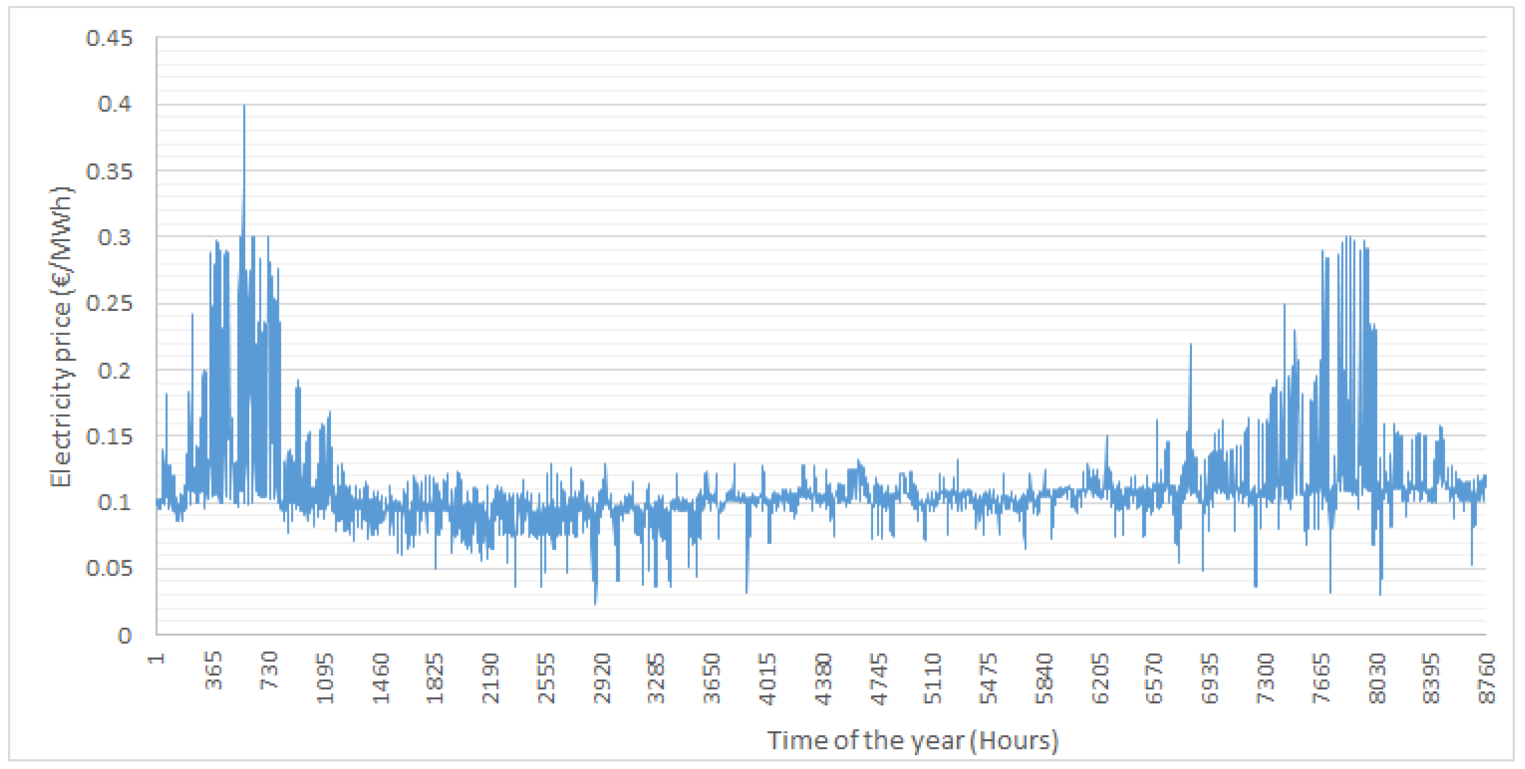
This section provides the results obtained for the considered operation scenarios. The main aim is to investigate the economic effects of the proposed charging strategy, the PV sizing and the PEV number penetration into the microgrid. The real time electricity prices of the first year are depicted in
Figure 10. It is assumed that the electricity price deviates ±5% every next year. Similarly, the PV production is assumed to deviate ±3% every next year.
Figure 11 depicts the Watt per installed PV kWp obtained from a PV installation of the examined area.
Table 2 lists the input data of the optimization problem. Further than that, the PV degradation every year is considered 0.6% [
28] and the efficiency of the DC/AC PV inverter is assumed to be 97.5%.
Five scenarios were considered regarding the number of the PEVs that would charge at the microgrid: (a) 100 PEVs, (b) 300 PEVs, (c) 500 PEVs, (d) 20 PEVs with 15% increase of their number every year and (e) 20 PEVs with 15% increase of their number every year, and only one-third of the PEV drivers would accept to participate in V2G.
Table 3 shows the NPV of the investment when the uncoordinated charging strategy is applied. The NPV is independent from the number of PEVs in this case as it examines the contribution only of the PV investment to the microgrid. Doubling the capacity of PV leads to a corresponding doubling of the NPV. The application of the proposed charging strategy can bring more profit to the microgrid as shown in
Table 4. In particular,
Table 4 summarizes the gains of the proposed charging strategy compared with the uncoordinated charging strategy when the PV is installed in the sport center at the end of investment period. The proposed algorithm is examined taking into consideration only the electricity price (s1) or the electricity price and the PV generation (s2). It can be observed that, as the number of the PEV increases, the profit is increasing as well. This happens because more PEVs participate in the V2G. More specifically, the energy can be sold back to the grid if there is a surplus of energy in the microgrid and the electricity price is high, or it can supply the microgrid. In this way, there is profit from selling the energy to the grid when the electricity price is high or the microgrid can reduce its demand during peak rates of the electricity price and subsequently increase its savings. Moreover, when s2 is applied the profits are increased more than 57%. It can be concluded that taking into consideration the electricity price and the PV generation could lead to better performance of the system. Furthermore, it can be observed that the profits in scenario e are almost 20% less than in scenario d even given the PEVs that were allowed to participate in V2G were one-third less in scenario e than in scenario d. This happened because Equation (1) should hold in order for a PEV to participate in V2G. Hence, a part of the PEV that was not allowed to participate in V2G in scenario e did not participate in V2G in scenario d either. Finally, in
Table 5 can be observed the payback period (PP) for the different scenarios. As the PV capacity is being increased, the PP of the proposed charging strategies tends to be same as the uncoordinated charging. On the other hand, as the number of the PEV is being increased the PP of the proposed charging strategies tends to be reduced compared to the uncoordinated charging. The increase of the PV capacity increases also the initial investment cost. In addition, the increase of the PEV number increases the profit from the smart charging process. Hence, the greater the increase in the number of electric vehicles and the lower the initial investment are, the shorter the payback period will be and vice versa.
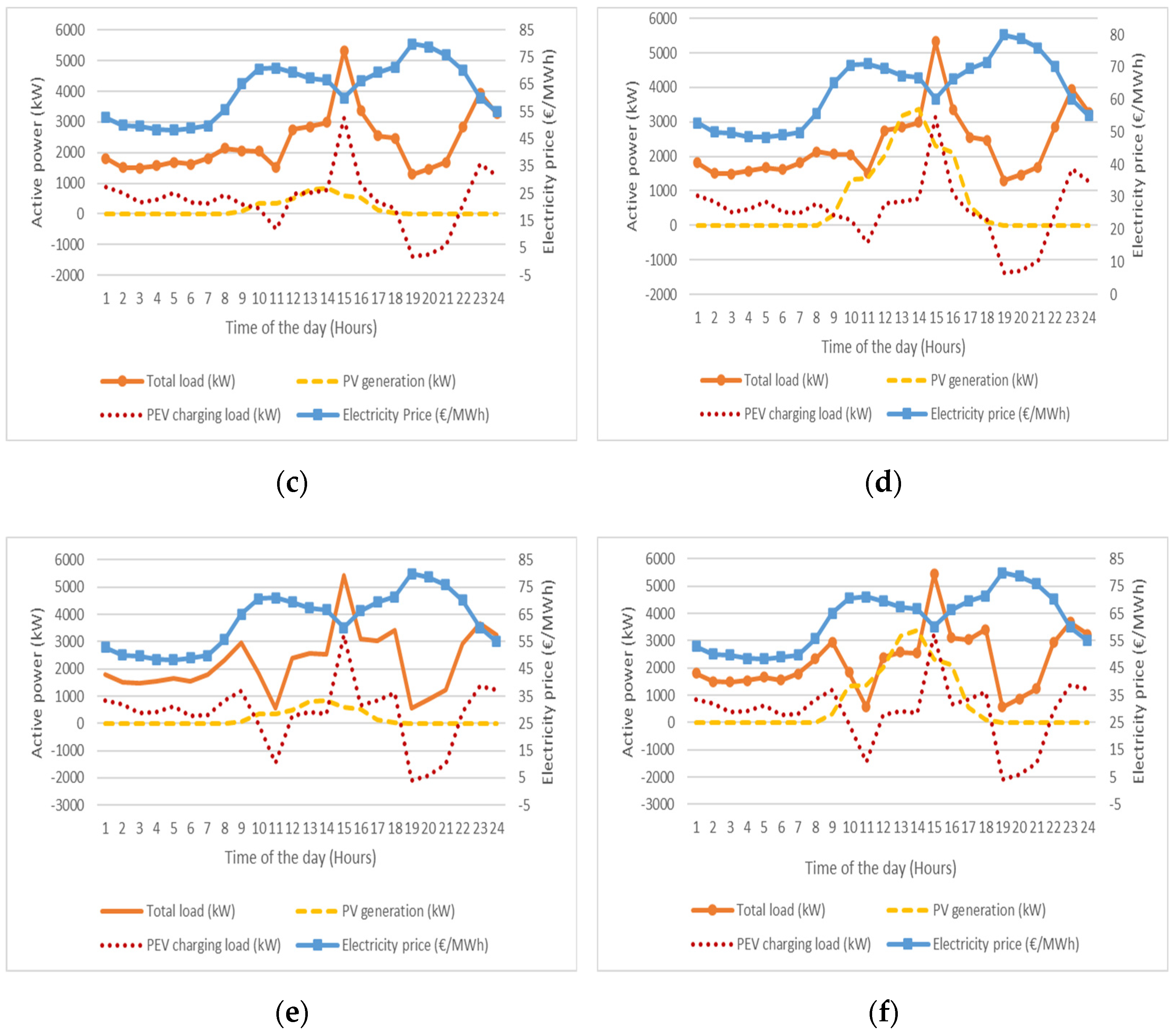
Figure 16 shows the daily electricity price, PV generation, PEV charging load and total load of the OAKA microgrid when the PEV number is 500 and for different PV generation and charging strategies. The number of PEVs that is selected to be demonstrated in
Figure 16 is 500 because their charging load is the highest and it can be observed better the influence of the PEV charging load on the microgrid total load curve. It can be observed that when the uncoordinated charging strategy is applied, the electricity price and the PV generation do not affect the total load of the microgrid as the PEV charges after they plug-in without taking into consideration any other factors (
Figure 16a,b). On the other hand, when s1 is applied, the PEV charging load influences the total demand of the microgrid significantly, as is shown in
Figure 16c,e. The peak demand of the microgrid is shifted during the time slots where the electricity price is low and new peak demand is created during the time slots where the electricity price is high. In addition, when the PV generation is introduced, s2, to the proposed charging strategy (
Figure 16d,f), a part of the charging load is shifted to the time slot where the PV generation is high, and the electricity price is low.
The assessment of the profitability of the PV investment in a microgrid equipped with PEV charger was examined in this study. The key finding from the results is that the application of a smart charging strategy and V2G can increase the NPV of the PV investment in a microgrid. In addition, the proposed charging algorithm can change the load curve when the PEV charging load is substantial, by scheduling the charging of the PEVs when the electricity price is low and the discharging when the electricity price is high, as shown in
Figure 16. Some limitations of the approach of this study are that the charging policies, the electricity price, the microgrid load, and the solar irradiation prediction remain constant during the investment lifetime.
Moreover, the charging policies play a significant role in the profits of the microgrid. In this study it is assumed that the profits of V2G will be collected from the microgrid. However, part of the profits could go to the PEV drivers. In addition, charging policies should take into consideration the cost of battery degradation caused by the participation of PEVs in V2G. Furthermore, not all drivers would accept to participate in V2G. Hence, the profit of the microgrid would be reduced. While the model considers the uncertainties of the electricity price, the microgrid load and the solar irradiation, no specific prediction model for the drivers’ incentives was used. These factors can potentially change the anticipated results. Finally, the arriving and departure of PEVs is assumed to be similar to the first year. The PEV consumption profile has a major effect on the optimization problem. The accuracy of this profile is able to render the study reliable enough. However, the stochastic behavior of PEV drivers cannot guarantee a perfectly accurate profile.


