Energy Consumption Prediction for Fused Deposition Modelling 3D Printing Using Machine Learning

Abstract

Additive manufacturing (AM) technologies are growing more and more in the manufacturing industry; the increase in world energy consumption encourages the quantification and optimization of energy use in additive manufacturing processes. Orientation of the part to be printed is very important for reducing energy consumption. Our work focuses on defining the most appropriate direction for minimizing energy consumption. In this paper, twelve machine learning (ML) algorithms are applied to model energy consumption in the fused deposition modelling (FDM) process using a database of the FDM 3D printing of isovolumetric mechanical components. The adequate predicted model was selected using four performance criteria: mean absolute error (MAE), root mean squared error (RMSE), R-squared (R2), and explained variance score (EVS). It was clearly seen that the Gaussian process regressor (GPR) model estimates the energy consumption in FDM process with high accuracy: R² > 99%, EVS > 99%, MAE < 3.89, and RMSE < 5.8.

1. Introduction

Additive manufacturing, or 3D printing, is defined as the material deposition process from computer-aided design (CAD) models, usually layer upon layer [1,2,3].

Additive manufacturing (AM) is widely applied in a broad spectrum of domains, including architecture, mechanics, aeronautics, chemical industry, education, food, social culture, and medicine [4,5]. Indeed, the importance of additive manufacturing importance has grown during the COVID-19 pandemic; several medical tools have been created to mitigate disruptions in the global medical field [6].

AM is a generic term for a group of processes which can be classified according to machine architecture into seven categories [7,8],

Table 1. Brief description of different additive manufacturing processes [7,8].

AM Process Type	Brief Description	Material Used	Technologies
Vat photopolymerization	photopolymers are exposed to repeated forms of radiation corresponding to cross sections of the part under construction.	Photopolymers	Stereolithography, digital light processing (DLP)
Powder bed fusion	Thermal energy selectively merges the regions of a powder bed.	Metals, polymers	Electron beam melting (EBM), selective laser sintering (SLS),selective heat sintering (SHS), direct metal laser sintering(DMLS)
Material extrusion	The melted material is selected through a nozzle.	Polymers	Fused deposition modelling (FDM)
Material jetting	Droplets of build material are placed selectively.	Polymers, waxes	Multi-jet modelling (MJM)
Binder jetting	A binder is printed onto a powder bed to form the part’s cross section.	Polymers, foundry sand, metals	Powder bed and inkjet head (PBIH), plaster-based 3D printing (PP)
Sheet lamination	Sheets of materials are cut, stacked, and bonded to form an object.	Paper, metals	Laminated object manufacturing (LOM), ultrasonic consolidation (UC)
Direct energy deposition	Thermal energy is used to merge materials by melting as the material is being deposited.	Metals	Laser metal deposition (LMD), electron beam metal deposition, wire arc additive manufacturing (WAAM)

summarized the different AM processes and associated technologies and materials.

As is evident, the range of techniques and materials is very wide. This subsector of additive manufacturing is growing rapidly in the industrial world, with compound annual growth rates of 24.5% [9,10], because additive manufacturing methods are more efficient and more flexible than conventional manufacturing methods, such as subtractive manufacturing and formative manufacturing. Therefore, attention is increasingly focused on the energy consumption of additive manufacturing (AM) systems. Much research has been conducted on energy consumption modeling for the AM process [10,11,12]. However, an efficient model for predicting energy consumption in the FDM process is still absent, in particular regarding the usage of machine learning (ML) for estimating energy use in the FDM process based on part orientation.

In this work, we mainly focus on energy consumption prediction in the fused deposition modelling (FDM) process. This process is one of the most frequently applied additive manufacturing methods. In fact, FDM printers largely simplify and accelerate the production process, providing users with an efficient manufacturing environment with better material utilization and reduced time consumption. The FDM principle is based on the extrusion of molten thermoplastic filaments layer by layer to form three-dimensional parts [13]. The FDM method includes numerous printing parameters, such as percentage infill, infill style, layer thickness, printing speed, and printing temperature, which affect the quality of the final product [14,15,16].

The aim of the current study is to model the experimental results of energy consumption for the FDM 3D printing of isovolumetric mechanical components using several ML algorithms. The simulation results provide the expected results and demonstrate the predictive accuracy of the Gaussian process regressor (GPR) method versus other ML methods used. With our developed GPR model, we can select the appropriate orientation of the part to be printed in order to reduce energy consumption. This prediction can be used to encourage engineers as they develop intuition for novel designs with FDM technology.

In this paper, the Section 2 presents a literature overview on energy consumption estimation in 3D printing. The Section 3 is devoted to the presentation of experimental data extracted from [11]. The Section 4 is dedicated to the methodologies of the ML algorithms used to model the energy consumption use of 3D printing isovolumetric mechanical components, while the prediction results and discussion are presented in the Section 5 and Section 6. The Section 7 presents conclusions.

2. Literature Review

A significant number of research studies investigated the estimation and the optimization of energy use in AM Processes by following various modeling approaches, such as mathematical and mechanical modeling, based on the process’s physics and artificial intelligence modeling.

A prediction model of energy consumption and printing time based on the working states of machine components and process parameters was proposed [17].The proposed model has certain limitations in the printing phase; the prediction model did not take into account the time needed for the empty travel, acceleration, and deceleration of the nozzle movement.

A data fusion method was suggested based on the convolutional neural network and long short-term memory CNN-LSTM model for AM energy consumption prediction [18]. For validating the proposed model, a case study was carried out using an SLS system. The CNN-LSTM-developed model does not predict accurately; this may be due to a significant loss of information during the convolution feature extraction process because the sliced images are less informative.

An energy consumption prediction model for AM systems was developed that incorporates clustering techniques and deep learning to integrate the multi-source data collected using the Internet of Things [19]. For validating the approach, a case study is conducted on the basis of actual data collected on the SLS process, which demonstrated the merits of the proposed approach.

In [20], authors presented the implementation of a tool to predict the energy flows occurring in direct metal laser sintering. A model for assessing energy and material consumption for binder jetting was developed [21]. A comparative study on energy consumption made at the process level for conventional and additive manufacturing processes was presented [22].

In [23], authors developed an approach based on the NC codes to estimate the material usage, time, and energy consumption of 3D-printed models. They validated their approach with two experiments, both of which present deviations of around 9% and 11% from the theoretical values.

A deep learning algorithm (ANN) was applied to predict the part mass, support material mass, and build time of voxelized objects for an AM process [24]. The results of the model were compared to results generated afterwards. This prediction model had low accuracy, with determination coefficients of 46.8% for part mass, 30.1% for support material mass, and 22.5% for build time.

A model and an energy profiler was developed to simulate the energy cost of the printing process [11]. From the obtained results, they suggested a cross-layer energy optimization solution, called 3DGates; it was assessed over 338 benchmarks on a 3D printer and realized a 25% reduction in energy consumption.

In [25], researchers built an energy consumption model and calculated the amount of energy used in wire-based additive–subtractive hybrid manufacturing and powder-based hybrid additive–subtractive manufacturing. They observed that the wire-based and powder-based methods used similar amounts of energy.

Potential environmental implications of AM were described in [26], such as energy use, waste, lifecycle impact, and occupational health, noting that AM technologies use more energy than conventional manufacturing technologies.

A mathematical model was developed for estimating the energy consumption of stereolithography processes [2].The obtained results were validated experimentally, the effects of different parameters on the total energy consumption was studied, and an optimization method was proposed to minimize energy consumption based on an optimal combination of parameters.

In [27], the operating procedure was analyzed and the impact of printing parameters on the energy consumption and particulates emissions was studied. The power profile analysis illustrated that print bed heating and temperature maintenance consume significant amount of energy during the FDM process.

Based on the abovementioned works, it is evident that a large amount of research has been performed on the estimation and optimization of the energy consumption of 3D printing processes. However, little work has been done to develop an efficient model based on part orientation to predict and minimize energy use in the FDM process. In this work, 12 ML models are used to select the most efficient model for obtaining the best prediction of energy consumption.

This paper has three main aims:

• Predict the energy use of FDM printed parts;
• Assess the impact of printing parameters on energy consumption;
• Optimize energy consumption based on the orientation of the part to be printed.

3. Design of Experiment Data

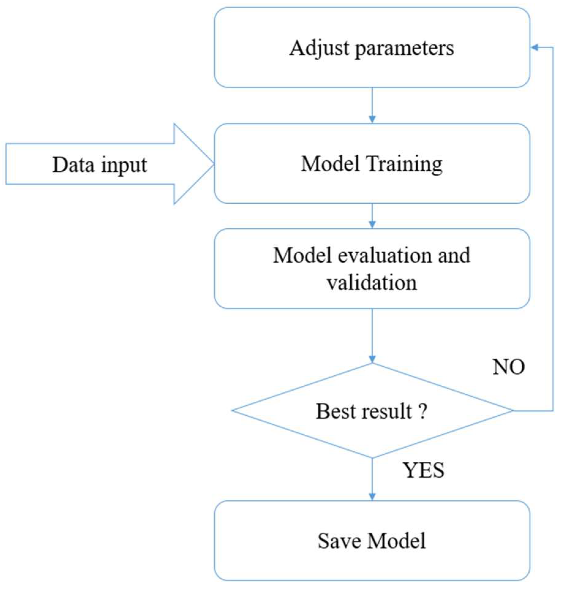
The data used in this research were retrieved from the experiment reported in [16]. We applied the machine learning algorithms to predict the energy consumption and compared it with the actual experimental results reported by the authors in [16]. The experiment was conducted using a Prusa i3 MK3S 3D printer. Electrical energy consumption was assessed for printing 68 different isovolumetric mechanical components with multiple orientations (total of 184 model files); these components were selected from Mechanical Components Benchmark (MCB) [28]. The experimental setup included four Adafruit INA260 sensors to measure the current consumption of the 3D printer, Arduino MKR WiFi 1010 to collect the electric current data from the current sensors, and a Raspberry Pi board to read the serial data coming from the Arduino board.

Many parameters affect the energy consumption in FDM 3D printing, including printing orientation of the model, stl surface area, number of facets, extrusion speed, extrusion temperature, sliced X’, sliced Y’, sliced Z’, sliced volume, sliced volume including support, total filament, percentage infill (20%), layer thickness, expected print time, and number of layers.

Extrusion speed and temperature are among the most important parameters affecting FDM printing; they have been used as recommended by the manufacturer [16]. Since extrusion speed, extrusion temperature, percentage infill, and layer thickness are constant parameters, they do not affect the learning phase, so we will not take these as input data.

The range of input parameters used is shown in

Table 2. Input parameters interval values.

Input Parameters	Intervals
Orientation	[0–180]
stl surface area	[1533.85–10,850.92]
Number of facets	[40–9368]
Sliced X	[3.23–153.87]
Sliced Y	[8.45–67.27]
Sliced Z	[3.23–153.87]
Sliced volume	[2142.39–5852.08]
Sliced volume including support	[2171.28–11,376.59]
Total Filament	[2.76–14.45]
Expected print time	[0.4166–4.033]
Number of layers	[21–1629]

[28].

The experimental data are used in this research to train machine learning algorithms to predict energy consumption in the FDM process.

4. Methodology

In this work, we aim to propose a model for predicting energy consumption in the FDM process. For this, before training the different algorithms that we will present afterwards, it is necessary to prepare and perform some processing on the dataset:

-

The first step is data cleaning, in which we eliminate the useless information to keep only the input and output parameters used in our study, which are shown in Table 2.

-

In the second step, we will transform the data into a format or structure that would be more appropriate for model development and also data exploration in general. In our case, we have used standard scaler.

After data processing, we train each algorithm using different parameters until we find the optimal parameter values for our data, as shown in Figure 1.

In this section, we will review the different machine learning algorithms that we have used to find the best model to predict energy consumption in the FDM process, using as input the data shown in Table 2. Then we will present the statistical indicators used to measure performance.

4.1. Overview of Machine Learning Algorithms

4.1.1. Linear Regression

The mathematical formula for linear regression [29,30] is defined by the following equation:

$$\begin{array}{l}\mathrm{E}(Y\mid X=x)={\beta }_0+{\beta }_{1}x\hfill \\ Var(Y\mid X=x)={\alpha }^2\hfill \end{array}$$

(1)

This linear regression model is formed by the mean function; it is a linear equation that combines a set of input values (X) with the output (Y) that represents the predicted value. The ${\beta }_0$ value is obtained for $\mathrm{E}(Y\mid X=x)$ with X = 0 and the intercept ${\beta }_1$ is calculated by changing the values of X. The variance is assumed to be a positive value, usually unknown.

The observed value and the estimated value are related by the following formula:

$$y_i=\mathrm{E}\left(Y\mid X=x_i\right)+e_i\mathrm{or}\mathrm{explicitly}\mathrm{by}{e}_i=y_i-\mathrm{E}\left(Y\mid X=x_i\right)$$

(2)

where $e_i$ is the error calculated in estimation, which depends directly on the unknown parameters.

4.1.2. RANSACRegressor (Random Sample Consensus)

RANSAC is a random sampling algorithm which was first introduced by Fischler and Bolles [31]. This algorithm gives a fit to the model by excluding outliers; RANSAC is able to smooth and interpret training data containing gross errors. The presence of outliers has an impact on the parameters of the training model, so it is preferable to remove outliers from the training. The objective of RANSCAN is to fit the model with outliers while efficiently exploring the parameter space to maximize an objective function $C$ (3). In the standard RANSAC formula, the maximized objective function $C$ is the support size for a given model. In other words, the support is the number of points that have residual errors below a predefined threshold t (4), and the group of points is called the consensus set. The goal of the method is to maximize the cardinal of this group (3).

$$C={\displaystyle \sum _i^{}\rho }\left(e_i^2\right)$$

(3)

$$\rho \left(e_i^2\right)=\{\begin{array}{ll}1\hfill & \mathrm{for}{e}_i^2\le t^2\hfill \\ 0\hfill & \mathrm{for}{e}_i^2>t^2\hfill \end{array}$$

(4)

4.1.3. Ridge Regression

This approach was introduced by Hoerl-Kennard [32]. It aims to optimize Formula (5):

$${\min }_{\beta }E(\alpha ,\beta )={\displaystyle \sum _{i=1}^n{(y_i-X_i\beta )}^2}+\alpha \Vert \beta {\Vert }^2$$

(5)

It is a linear regression with quadratic constraint on the coefficients. This regression is used more when we have variables that are highly correlated. The solution can be expressed as follows:

$${\mathsf{\beta }}^{*}{=(\mathrm{X}\text{′}\mathrm{X}+\mathsf{\alpha }\mathrm{I})}^{-1}\mathrm{X}\text{′}\mathrm{Y}$$

(6)

where ${\mathsf{\beta }}^{*}$ is the estimator of $\mathsf{\beta }$, matrix $\mathsf{\alpha }\mathrm{I}$ is a named bias factor, and it is possible to choose an $\alpha$ for which the matrix $(X^{\prime }X+\alpha I)$ is invertible. This is especially useful when there are several variables. The goal of Hoerl-Kennard is to make the matrix $(X^{\prime }X+\alpha I)$ invertible; the higher the value of α, the more robust the model coefficients.

4.1.4. Lasso Regression

This is a regression technique with coefficient constraint. It is used when the variables have a high correlation. This method is very effective, especially with a database that has a large dimension [33]. Lasso regression aims at optimizing Problem (7):

$${\min }_{\beta }E(\alpha ,\beta )={\displaystyle \sum _{i=1}^n{(y_i-X_i\beta )}^2}+\alpha \Vert \beta \Vert$$

(7)

For a single variable, this regression acts on one variable, and lasso must minimize the following formula:

$$E(\beta )={\displaystyle \sum _{i=1}^n{(y_i-\beta x_i)}^2}+\alpha |\beta |$$

(8)

That is, we must find $\beta$ with $E(\beta )=0$

In other words:

$$E^{\prime }(\beta )=\{\begin{array}{ll}{\displaystyle \sum _{i=1}^n-}{x}_i(y_i-\beta x_i)+\alpha \hfill & \mathrm{si}\beta >0\hfill \\ {\displaystyle \sum _{i=1}^n-}{x}_i(y_i-\beta x_i)-\alpha \hfill & \mathrm{si}\beta <0\hfill \end{array}$$

(9)

$$And:E^{\prime }(\beta )=0\iff \{\begin{array}{ll}\beta =\frac{-\alpha +{\displaystyle \sum _{i=1}^n{x}_i}{y}_i}{{\displaystyle \sum _{i=1}^n{x}_i^2}}\hfill & \mathrm{si}\beta >0\hfill \\ \beta =\frac{\alpha +{\displaystyle \sum _{i=1}^n{x}_i}{y}_i}{{\displaystyle \sum _{i=1}^n{x}_i^2}}\hfill & \mathrm{si}\beta <0\hfill \end{array}$$

(10)

4.1.5. Gaussian Process Regressor (GPR)

The Gaussian process regressor formula is given by (13) with the input $X=\left[x_1,x_2,\dots ,x_n\right]$, the output $Y=\left[y_1,y_2,\dots ,y_n\right]$, and for any element $\left\{\left(x_i,y_i\right)\mid i=1,\dots ,n\right\},$$y_i=f\left(x_i\right).$ The main idea of GPR is to apply a Gaussian process (GP) to represent f(x), which we will call latent variables. Input X allows us to index these latent variables so that $\left\{f\left(x_1\right),\dots ,f\left(x_k\right)\right\}$ is a Gaussian distribution correlated between all elements.

$$\mathrm{m}\left(\mathrm{x}\right)=\mathrm{E}\left(\mathrm{f}\right(\mathrm{x}\left)\right)$$

(11)

m(x) is the mean of f(x) and, for the covariance, is described by the following equation:

$$k\left(x,x^{\prime }\right)=E(f(x)-m(x))\left(f\left(x^{\prime }\right)-m\left(x^{\prime }\right)\right)$$

(12)

$\mathrm{E}\left(\right)$ represents the expectation. The function of the mean is especially important when there is a region with unobserved inputs with a value of zero.

The Gaussian process regressor is given by:

$$f\left(x\right)~GP(m(x)，k(x，x^{\prime }))$$

(13)

with:

$$y_i=f\left(x_i\right)+\epsilon$$

(14)

$\epsilon ~N\left(0,{\sigma }^2\right)$ and ${\sigma }^2$ are the variance of the noise.

For the covariance, there are some specific parameters that are independent and give the distribution of $\mathrm{f}\left(\mathrm{X}\right)$ and named hyperparameters ${\theta }_i^{}$, and it usually uses the exponential squared Covariance (15).

$$k\left(x,x^{\prime }\right)={\theta }_1\exp \left(-\frac{{\Vert x-x^{\prime }\Vert }^2}{2{\theta }_2}\right)$$

(15)

Note that the covariance function decreases rapidly at input pairs x and x’, which are distant, which expresses a low correlation between f(x) and f(x’). Therefore, ${\theta }_1^{}$ is a hyperparameter that represents the maximum correlation and ${\theta }_2^{}$ is a positive value defining the rate of decline for the correlation of points that are not close to each other.

4.1.6. Elastic Net Regressor

The elastic net regression model was introduced by [34] in order to solve the criticisms on the lasso, whose set of selection variables may be too dependent on the data and therefore unstable. The solution is to combine the regression penalties of ridge regression and lasso to exploit the best aspects of both methods. Elastic net aims to minimize Function (16):

$$L_{\mathrm{enet}}(\widehat{\beta })=\frac{{\displaystyle \sum _{i-1}^n{\left(y_i-x_i^{\prime }\widehat{\beta }\right)}^2}}{2n}+\lambda \left(\frac{1-\alpha }{2}{\displaystyle \sum _{j=1}^m{\widehat{\beta }}_j^2}+\alpha {\displaystyle \sum _{j=1}^m\left|{\widehat{\beta }}_j\right|}\right)$$

(16)

with:$\widehat{y}={\widehat{\beta }}_0+x_1{\widehat{\beta }}_1+\cdots +x_n{\widehat{\beta }}_n$ is the predicted value for the input X of n elements.

${\widehat{\beta }}_i$ is the predicted coefficient.

$0 \le \alpha \le 1$ and $\lambda \ge 0$

where α is the mixing parameter between ridge regression (α = 0) and the lasso (α = 1). Here, $\alpha$ determines the influence of ridge regression relative to lasso.

There are two parameters to adjust: λ (penalty) and α.

Elastic net must minimize the following function [34]:

$$EN(\beta )={\displaystyle \sum _{i=1}^n{\left(y_i-x_i^{\top }\beta \right)}^2}+{\lambda }_1{\displaystyle \sum _{j=1}^p\left|{\beta }_j\right|}+{\lambda }_2{\displaystyle \sum _{j=1}^p{\left|{\beta }_j\right|}^2}$$

(17)

where ${\lambda }_1$ and ${\lambda }_2$ are the lasso and ridge regression penalties, respectively.

Elastic net combines the advantages of lasso and ridge, which are shrinkage and sparsity, respectively.

4.1.7. Random Forest Regressor

This approach has a set of regression trees, and a sample of the training is processed each time first. In other words, each sample produces a regression tree. For the prediction of the test data, the average of the predictions of each tree is calculated; each tree gives us a prediction, and the prediction result is the average of the values (18).

$$RF(X)={\displaystyle \sum _{i=1}^p{T}_i}(X)$$

(18)

The algorithm of this approach is the following:

• Step 1: From the dataset, we choose N records at random.
• Step 2: For each N records, we create a regression tree.
• Step 3: For each tree, we repeat steps 1 and 2.
• Step 4: For a problem of a record E, we take the average of the other predictions of the other trees to estimate the Y value of the output.

4.1.8. SVM

SVM was introduced by Vapnik [35]. The SVM regression method is given by Formula (19), in which φ(x) is a nonlinear mapping function of the input x into a feature space and the two respective parameters b and ω represent the weight vector and a coefficient, respectively, both of which are to be calculated from the data. By performing a linear regression in a high dimensional feature space with nonlinear mapping, the two parameters b and ω are estimated by minimizing Sum (20), in which C is a constant and positive value that determines the tradeoff between the complexity of the model and the sum with a condition of having an error greater than ε. ||ω||² is the Euclidean norm of the regression vector ω, and Lε is a loss function that calculates the empirical risk R (20).

$$f(x)=\omega \cdot \varphi (x)+b$$

(19)

$$R=C{\displaystyle \sum _{i=1}^n{L}_{\epsilon }}\left(f\left(x_i\right),y_i\right)\frac{1}{2}\Vert \omega {\Vert }^2$$

(20)

$$L_{\epsilon }\left(f\left(x_i\right),y_i\right)=\{\begin{array}{ll}0\hfill & \mathrm{for}\left|f\left(x_i\right)-y_i\right|<\epsilon \hfill \\ |f(x)-y|-\epsilon \hfill & \mathrm{otherwise}\hfill \end{array}$$

(21)

4.1.9. Multi-Output Regression—SVR

This regression method [36] was introduced by Pérez-Cruz et al. [37]. This method is more generalized than standard SVR. Considering the $\left\{{\phi }_1,{\phi }_2,\dots ,{\phi }_N\right\}$ time series and for the multi-step prediction and modeling, this amounts in other words to finding in training the relation between the value of the previous observation x and the current observation y with: $x=\left[{\phi }_t,{\phi }_{t-1},\dots ,{\phi }_{t-d+1}\right]\in {ℝ}^d$ and $y=\left[{\phi }_{t+1},{\phi }_{t+2},\dots ,{\phi }_{t+H}\right]\in {ℝ}^H$; i.e., for ${\left\{\left({\mathrm{x}}_i,{\mathrm{y}}_i\right)\right\}}_{i=d}^n$, the M-SVR aims to find a $w^j$ regressor and also find $b^j(j=1,\dots ,H)$ for each output by minimizing:

$$L_p(W,b)=\frac{1}{2}{\displaystyle \sum _{j-1}^H|}|w^j|{|}^2+C{\displaystyle \sum _{i=1}^{n}L}\left(u_i\right)$$

(22)

with: $u_i=\Vert e_i\Vert =\sqrt{\left(e_i^T{e}_i\right)}$ and

$$e_i^T=y_i^T-\phi \left(x_i\right)W-b^{T}W=\left[w^1,\dots ,w^H\right],b={\left[b^1,\dots ,b^H\right]}^T$$

(23)

where $C$ is a parameter that determines the relationship between the regressor $w^j$ and the error $e_i^{}$ and $\phi (.)$, a nonlinear function to the feature space $x$. $L(u)$ is a quadratic cost function that is independent at epsilon:

$$L(u)=\{\begin{array}{ll}0\hfill & u<\epsilon \hfill \\ u^2-2u\epsilon +{\epsilon }^2\hfill & u\ge \epsilon \hfill \end{array}$$

(24)

This approach is called support vector regression and was developed to perform regression [36]. The specificity of this method is that the training is performed only on a subset of the data. This is done given the cost for building the model; the SVR takes only the training data that are not close (with respect to a threshold e).

Multi-output regression is widely used, especially the objective is to make simultaneous predictions of several values in output. SVRs are more efficient than time series because the latter do not provide reassuring results for non-linear data.

4.1.10. Regression Chain

This method is based on the classical chain classification method. RC has the advantage of chaining models to a single target variable while creating regression models for each of the variables, which allows us to build in sequential order a chain of targets. The first target variable related to the regression model to be built is chosen independently from the other target variables. In the prediction process, these target values become inputs to the training set to predict the next target variable. That is, for X as input and for Y as output with three target variables Y (y1, y2, and y3) in the first regression, we fit the first model M1 for the variable y1 taking X as input (25). The second iteration concerns the second model, M2, which will be adjusted for the target variable y2 based on the training set, which is X and y1 (26), so model M3 is adjusted in the same way while having X and y1 and y2 as inputs (27).

$$(\mathrm{X}, \mathrm{y}\mathrm{1}) \to \mathrm{M}\mathrm{1}$$

(25)

$$(\mathrm{X} \mathrm{e}\mathrm{t} \mathrm{y}\mathrm{1},\mathrm{y}\mathrm{2}) \to \mathrm{M}\mathrm{2}$$

(26)

$$(\mathrm{X},\mathrm{y}\mathrm{1} \mathrm{e}\mathrm{t} \mathrm{y}\mathrm{2},\mathrm{y}\mathrm{3}) \to \mathrm{M}\mathrm{3}$$

(27)

4.1.11. KNeighbors Regressor

KNeighborsRegressor it is a supervised technique in machine learning. It is based on the neighbors; the KNN consists of performing a regression for the continuous labels. This method is based on the measure of similarity between the nearest elements. This measure is obtained by using the Euclidean distance between the nearest values (28).

$$d=\sqrt{{\displaystyle \sum _{i=1}^n{(yi-xi)}^{\wedge }}2}$$

(28)

The value of K is calculated in training. It must not be very small in order to not overfit the regression model and to avoid noise in the model. In other words, the value of K is determined in order to obtain the best model.

4.1.12. DecisionTreeRegressor

This is a supervised machine learning technique used for both classification and regression. This approach is based on the decision tree [21]. It is useful to train the data in a tree-like way and to make predictions.

4.2. Evaluation Metrics

In order to evaluate the performance of the approaches used, four statistical indicators were calculated: MAE (mean absolute error), RMSE (root mean square error), R² Square (coefficient of determination), and ESV (explained variance score):

• Mean absolute error (MAE) is the mean of the absolute value of the errors; this indicator represents the average of the absolute difference between the actual and predicted values in the database. It measures the average of the residuals in the data set (29).

$$MAE=\frac{1}{N}{\displaystyle \sum _{i=1}^N|}{y}_i-\widehat{y}|$$

(29)

$\begin{array}{l}\widehat{y}-\mathrm{predicted}\mathrm{value}\hfill \\ \overline{y}-\mathrm{mean}\mathrm{value}\hfill \end{array}$

• Root mean squared error (RMSE); this measure represents the root mean square error of the squared difference between the original and predicted values of the model (30).

$$RMSE=\sqrt{\frac{1}{N}{\displaystyle \sum _{i=1}^N{(y_i-\widehat{y})}^2}}$$

(30)

• R-Squared expresses the ratio of the variance of the variable explained by the model with the original value (31).

$$R^2=1-\frac{{\displaystyle \sum _{}^{}{(y_i-\widehat{y})}^2}}{{\displaystyle \sum _{}^{}{(y_i-\overline{y})}^2}}$$

(31)

Explained variance score (EVS); this metric expresses the rate representing the variance of the current value (true value) and the estimated value (32).

$$\mathrm{Explained}\mathrm{variance}\left(\mathrm{y},\widehat{y}\right)=1-\frac{\mathrm{Var}\left(\mathrm{y}-\widehat{y}\right)}{\mathrm{Var}\left(\mathrm{y}\right)}$$

(32)

5. Results

In this article, we used twelve algorithms to find the most effective model for predicting energy consumption from the input (Table 2). Figure 2 shows a graphical comparison between the actual energy values and the predicted energy for each part and according to its different orientations using these algorithms.

Figure 2 shows that some models predict results closer to the actual values.

Table 3. Evaluation Metrics of used models.

	Model	MAE	RMSE	R-Squared	Explained Variance
1	Linear Regression	5.251029	11.569446	0.965963	0.969285
2	RANSACRegressor	5.167925	10.929534	0.969624	0.973401
3	Ridge Regression	5.894558	13.867725	0.951097	0.956034
4	GaussianProcessRegressor	3.881234	5.793596	0.991465	0.991602
5	Lasso Regression	5.764058	13.284901	0.955121	0.960033
6	Elastic Net Regression	5.920195	14.095655	0.949476	0.954896
7	Random Forest Regressor	7.287192	19.347954	0.904808	0.904854
8	SVM Regressor	9.683700	23.169309	0.863493	0.877995
9	Linear SVR Multi Output Regressor	15.571200	22.334431	0.873154	0.893362
10	Linear SVR Chain Regressor	15.588542	22.311816	0.873410	0.893883
11	KNeighborsRegressor	13.197450	24.191009	0.851189	0.851421
12	DecisionTreeRegressor	9.929268	23.336388	0.861517	0.862568

presents the statistical performance indicators for each model in terms of MAE, RMSE, R², and explained variance

Figure 3 illustrates the trend line between the actual and the predicted values of each prediction algorithm.

From Figure 3 and Table 3, it is clear that the GPR model achieves the highest precision, having 99.16% as the explained variance value. For the R-squared, it is 99.14%. The respective values of MAE and RMSE are 3.88 and 5.79. It can be seen that these values are the best in comparison with the other models.

6. Discussion

The benefits of artificial intelligence and machine learning algorithms in 3D printing are wide-ranging. In our case, before each printing, we will predict the printing energy depending on the part’s orientation. Figure 4 illustrates a graphical comparison between the actual energy values and the predicted energy for each part and according to its different orientations using the GPR model. It is clear that the two curves perform in a similar manner, so we can use the GPR model to find the best part orientation for printing, which will use less energy.

To assess the performance of our approach, four parts from the database were selected at random. For each part (

Table 4. Examples of comparison between actual energy and predicted energy by GPR.

Part	Orientation	Predicted Energy by GPR	Actual Energy
	0	70.01837754	76.969
	90	97.62380459	92.866
	180	196.11750589	143.278
	0	44.3041344	90.218
	90	158.10571579	138.686
	180	166.36283187	133.051
	0	78.20556709	89.38
	90	185.35942611	96.941
	180	98.38320959	90.133
	0	77.05352922	67.718
	90	203.28819197	141.432
	180	86.72962282	75.973

), we will predict the energy needed for printing according to the three orientations (0, 90, and 180).

From the results shown in Table 4:

• o For part number one, if we print it following orientation 180 instead of printing it following 0, we will lose about 70 Wh of energy.
• o For part number two, if we print it following orientation 90 instead of printing it following 0, we will lose about 50 Wh of energy.
• o For part number three, if we print it following orientation 90 instead of printing it following 0, we will lose about 7 Wh of energy.
• o For part number four, if we print it following orientation 90 instead of printing it following 0, we will lose about 90 Wh of energy.

These pertinent results confirm the capacity of our model based on the GPR algorithm to predict energy consumption in the FDM process with high accuracy.

7. Conclusions

In this research, twelve machine learning algorithms are used to model and predict energy consumption in the FDM process using a database of the FDM 3D printing of isovolumetric mechanical components (r3DIM benchmark). The most effective model is chosen based on four performance criteria: mean absolute error (MAE), root mean squared error (RMSE), R-squared (R2), and explained variance score (EVS). The GPR model outperformed these models with a high degree of accuracy and had the following performances: 99.16% as the value of explained variance and 99.14% for R-squared; the respective values of MAE and RMSE are 3.88 and 5.79, respectively. With our model, before each printing, we will be able to predict the printing energy according to different part orientations, and after the comparison between the predicted energies, we can decide the best orientation to use to minimize energy use in the printing phase.

References

1. ASTM-F2792-12a; Terminology for Additive Manufacturing Technologies. F42 Committee. ASTM International: West Conshohocken, PA, USA, 2012. [CrossRef]
2. Yang, Y.; Li, L.; Pan, Y.; Sun, Z. Energy Consumption Modeling of Stereolithography-Based Additive Manufacturing Toward Environmental Sustainability. J. Ind. Ecol. 2017, 21, S168–S178. [Google Scholar] [CrossRef] [Green Version]
3. Huang, R.; Riddle, M.; Graziano, D.; Warren, J.; Das, S.; Nimbalkar, S.; Cresko, J.; Masanet, E. Energy and emissions saving potential of additive manufacturing: The case of lightweight aircraft components. J. Clean. Prod. 2016, 135, 1559–1570. [Google Scholar] [CrossRef] [Green Version]
4. Kellens, K.; Baumers, M.; Gutowski, T.G.; Flanagan, W.; Lifset, R.; Duflou, J. Environmental Dimensions of Additive Manufacturing: Mapping Application Domains and Their Environmental Implications. J. Ind. Ecol. 2017, 21, S49–S68. [Google Scholar] [CrossRef] [Green Version]
5. Giannatsis, J.; Dedoussis, V. Additive fabrication technologies applied to medicine and health care: A review. Int. J. Adv. Manuf. Technol. 2007, 40, 116–127. [Google Scholar] [CrossRef]
6. Salmi, M.; Akmal, J.S.; Pei, E.; Wolff, J.; Jaribion, A.; Khajavi, S.H. 3D Printing in COVID-19: Productivity Estimation of the Most Promising Open Source Solutions in Emergency Situations. Appl. Sci. 2020, 10, 4004. [Google Scholar] [CrossRef]
7. Verhoef, L.A.; Budde, B.W.; Chockalingam, C.; Nodar, B.G.; van Wijk, A.J. The effect of additive manufacturing on global energy demand: An assessment using a bottom-up approach. Energy Policy 2018, 112, 349–360. [Google Scholar] [CrossRef]
8. Gibson, I. Additive Manufacturing Technologies, 3rd ed.Springer: New York, NY, USA, 2021. [Google Scholar]
9. Wohlers, T.T.; Associates, W.; Campbell, I.; Huff, R.; Diegel, O.; Kowen, J. 3D Printing and Additive Manufacturing State of the Industry. In Wohlers Report 2019; Wohlers Associates Inc.: Fort Collins, CO, USA, 2019. [Google Scholar]
10. Hopkins, N.; Jiang, L.; Brooks, H. Energy consumption of common desktop additive manufacturing technologies. Clean. Eng. Technol. 2021, 2, 100068. [Google Scholar] [CrossRef]
11. Ajay, J.; Song, C.; Rathore, A.S.; Zhou, C.; Xu, W. 3DGates: An Instruction-Level Energy Analysis and Optimization of 3D Printers. In Proceedings of the Twenty-Second International Conference on Architectural Support for Programming Languages and Operating Systems, Xi’an, China, 8–12 April 2017; pp. 419–433. [Google Scholar] [CrossRef] [Green Version]
12. Weissman, A.; Gupta, S.K. Selecting a Design-Stage Energy Estimation Approach for Manufacturing Processes. In Proceedings of the ASME 2011 International Design Engineering Technical Conference & Computers and Information in Engineering Conference IDETC/CIE 2011, Washington, DC, USA, 28–31 August 2011; pp. 1075–1086. [Google Scholar] [CrossRef] [Green Version]
13. Song, R.; Telenko, C. Material and energy loss due to human and machine error in commercial FDM printers. J. Clean. Prod. 2017, 148, 895–904. [Google Scholar] [CrossRef]
14. Sood, A.K.; Ohdar, R.K.; Mahapatra, S.S. Experimental investigation and empirical modelling of FDM process for compressive strength improvement. J. Adv. Res. 2012, 3, 81–90. [Google Scholar] [CrossRef] [Green Version]
15. Singh, S.; Singh, G.; Prakash, C.; Ramakrishna, S. Current status and future directions of fused filament fabrication. J. Manuf. Process. 2020, 55, 288–306. [Google Scholar] [CrossRef]
16. Szemeti, G.; Ramanujan, D. An Empirical Benchmark for Resource Use in Fused Deposition Modelling 3D Printing of Isovolumetric Mechanical Components. Procedia CIRP 2022, 105, 183–191. [Google Scholar] [CrossRef]
17. Yan, Z.; Huang, J.; Lv, J.; Hui, J.; Liu, Y.; Zhang, H.; Yin, E.; Liu, Q. A New Method of Predicting the Energy Consumption of Additive Manufacturing considering the Component Working State. Sustainability 2022, 14, 3757. [Google Scholar] [CrossRef]
18. Hu, F.; Qin, J.; Li, Y.; Liu, Y.; Sun, X. Deep Fusion for Energy Consumption Prediction in Additive Manufacturing. Procedia CIRP 2021, 104, 1878–1883. [Google Scholar] [CrossRef]
19. Qin, J.; Liu, Y.; Grosvenor, R. Multi-source data analytics for AM energy consumption prediction. Adv. Eng. Inform. 2018, 38, 840–850. [Google Scholar] [CrossRef]
20. Baumers, M.; Tuck, C.; Wildman, R.; Ashcroft, I.; Rosamond, E.; Hague, R. Transparency Built-In. J. Ind. Ecol. 2012, 17, 418–431. [Google Scholar] [CrossRef]
21. Meteyer, S.; Xu, X.; Perry, N.; Zhao, Y.F. Energy and Material Flow Analysis of Binder-jetting Additive Manufacturing Processes. Procedia CIRP 2014, 15, 19–25. [Google Scholar] [CrossRef] [Green Version]
22. Yoon, H.-S.; Lee, J.-Y.; Kim, H.-S.; Kim, M.-S.; Kim, E.-S.; Shin, Y.-J.; Chu, W.-S.; Ahn, S.-H. A comparison of energy consumption in bulk forming, subtractive, and additive processes: Review and case study. Int. J. Precis. Eng. Manuf. Technol. 2014, 1, 261–279. [Google Scholar] [CrossRef]
23. Yang, J.; Liu, Y. Energy, time and material consumption modelling for fused deposition modelling process. Procedia CIRP 2020, 90, 510–515. [Google Scholar] [CrossRef]
24. McComb, C.; Meisel, N.; Simpson, T.W.; Murphy, C. Predicting Part Mass, Required Support Material, and Build Time via Autoencoded Voxel Patterns. In Proceedings of the 2018 Annual International Solid Freeform Fabrication Symposium, Austin, TX, USA, 13–15 August 2018. [Google Scholar] [CrossRef] [Green Version]
25. Jackson, M.A.; Van Asten, A.; Morrow, J.D.; Min, S.; Pfefferkorn, F.E. A Comparison of Energy Consumption in Wire-based and Powder-based Additive-subtractive Manufacturing. Procedia Manuf. 2016, 5, 989–1005. [Google Scholar] [CrossRef] [Green Version]
26. Rejeski, D.; Zhao, F.; Huang, Y. Research needs and recommendations on environmental implications of additive manufacturing. Addit. Manuf. 2018, 19, 21–28. [Google Scholar] [CrossRef] [Green Version]
27. Simon, T.R.; Lee, W.J.; Spurgeon, B.E.; Boor, B.E.; Zhao, F. An Experimental Study on the Energy Consumption and Emission Profile of Fused Deposition Modeling Process. Procedia Manuf. 2018, 26, 920–928. [Google Scholar] [CrossRef]
28. r3DiM Benchmark. Available online: https://www.kaggle.com/dataset/c22f9996866156344599fd5baf48aaa8ac8ccce9a849b050ceeea36ba4e9c8f9 (accessed on 22 June 2022).
29. Weisberg, S. Applied Linear Regression, 3rd ed.Wiley: Hoboken, NJ, USA, 2005. [Google Scholar]
30. Maulud, D.; AbdulAzeez, A.M. A Review on Linear Regression Comprehensive in Machine Learning. J. Appl. Sci. Technol. Trends 2020, 1, 140–147. [Google Scholar] [CrossRef]
31. Fischler, M.A.; Bolles, R.C. Random sample consensus: A Paradigm for Model Fitting with Applications to Image Analysis and Automated Cartography. Commun. ACM 1981, 24, 381–395. [Google Scholar] [CrossRef]
32. Hoerl, A.E.; Kennard, R.W. Ridge Regression: Biased Estimation for Nonorthogonal Problems. Technometrics 1970, 12, 55. [Google Scholar] [CrossRef]
33. Van de Geer, S.A. High-dimensional generalized linear models and the lasso. Ann. Stat. 2008, 36. [Google Scholar] [CrossRef]
34. Zou, H.; Hastie, T. Regularization and Variable Selection via the Elastic Net. J. R. Stat. Soc. Ser. B Stat. Methodol. 2005, 67, 301–320. [Google Scholar] [CrossRef] [Green Version]
35. The Nature of Statistical Learning Theory. Available online: https://link.springer.com/book/10.1007/978-1-4757-3264-1 (accessed on 22 June 2022).
36. Kernel Methods for Pattern Analysis. Available online: https://www.cambridge.org/core/books/kernel-methods-for-pattern-analysis/811462F4D6CD6A536A05127319A8935A (accessed on 22 June 2022).
37. Pérez-Cruz, F.; Camps-Valls, G.; Soria-Olivas, E.; Pérez-Ruixo, J.J.; Figueiras-Vidal, A.R.; Artés-Rodríguez, A. Multi-dimensional Function Approximation and Regression Estimation. In Proceedings of the International Conference on Artificial Neural Networks, ICANN ’02, Lecture Notes in Computer Science. Madrid, Spain, 28–30 August 2002; Dorronsoro, J.R., Ed.; Springer: Berlin/Heidelberg, Germany, 2002; Volume 2415, pp. 757–762. [Google Scholar] [CrossRef]
Figure 1. Approach used to adjust parameters.
Asi 05 00086 g001
Figure 2. Actual and predicted energy values for each part.
Asi 05 00086 g002
Figure 3. Actual versus predicted values of each prediction algorithm.
Asi 05 00086 g003
Figure 4. Actual versus predicted values by GPR for each part.
Asi 05 00086 g004