Machine Learning Based Surrogate Models for the Thermal Behavior of Multi-Plate Clutches

Abstract

Multi-plate clutches play safety-critical roles in many applications. For this reason, correct functioning and safe operation are essential. Spontaneous damages are particularly critical because the failure of the clutch can lead to a failure of the system. Such damage mainly occurs due to very high loads and ultimately very high temperatures. Finite Element Analysis (FEA) enables simulation and prediction of these temperatures, but it is very time-consuming and costly. In order to reduce this computational effort, surrogate models can be created using machine learning (ML) methods, which reproduce the input and output behavior. In this study, various ML methods (polynomial regression, decision tree, support vector regressor, Gaussian process and neural networks) are evaluated with respect to their ability to predict the maximum clutch temperature based on the loads of a slip cycle. The models are examined based on two use cases. In the first use case, the axial force and the speed are varied. In the second use case, the lining thickness is additionally modified. We show that ML approaches fundamentally achieve good results for both use cases. Furthermore, we show that Gaussian process and backpropagation neural network provide the best results in both cases and that the requirement to generate predictions during operation is fulfilled.

1. Introduction

1.1. Motivation

Wet multi-plate clutches are machine elements in widespread use which are extensively employed in drive technology [1,2]. Applications range from starting and powershifting elements in dual-clutch and automatic transmissions, differential locks and torque converter clutches to serving as braking components in construction machinery or marine transmissions [3,4]. Given the nature of these applications and the high stresses that such components experience, multi-plate clutches fulfill safety-relevant roles, so safe and reliable operation must be ensured [5].

The damage and failures encountered during operation of multi-plate clutches can fundamentally be divided into two categories. Long-term damage refers to deterioration caused by variations in the friction system throughout a large number of shifting cycles. The number of shiftings until damage or failure can sometimes amount to several tens of thousands of shiftings. The latter category consists of spontaneous failures. These occur in individual shifting operations due to very high thermal and mechanical loads [4]. Since this phenomenon does not build up over time and therefore occurs unexpectedly, it is particularly critical and safety-relevant, because a single shift can jeopardize the safety of the entire system [6,7]. When considering damage to clutch systems, one key parameter is the maximum temperature within the plates and the friction lining, as these are ultimately responsible for the damage mechanisms. The temperatures during operation can be measured experimentally via sensors, which is often impossible due to the given design, the high experimental effort and the high costs, or temperatures can be simulated using finite element models. The disadvantage of the estimation through simulations is the high computational effort, which can be very resource- and time-intensive. As a result, FE simulations are not suitable for use during operation since a sufficient degree of real-time performance cannot be achieved.

One option for reducing computational effort is the use of surrogate models, which are also called meta-models. Surrogate models are simpler models that approximate the original models’ input–output behavior, but require much less computational effort than the original model [8]. Particularly interesting is the tradeoff between the accuracy of the calculations and the computational effort required by models [9]. For this reason, such models are very popular and extensively researched in various engineering fields, especially using such models in combination with FE models [9]. Two application areas of machine learning-based surrogate models are of particular interest: the use during development and design optimization and the prediction of relevant metrics during operation.

ML techniques related to the construction of surrogate models are applied in several areas. The field of structural mechanics in particular has already been the subject of many research projects combining FE and ML. Both classical machine learning methods and neural networks are finding extensive applications in the field. Hoffer et al. [10] investigated and compared the potential of gradient-boosting decision trees, k-nearest neighbor regressors, Gaussian processes, support vector regressors, and (physics-informed) neural networks for creating surrogate models of structural mechanics FE simulations based on three separate use cases. Badarinath et al. [9] employed decision tree-based methods and neural networks to predict the behavior of time-varying mechanical systems. The time-dependent stress of a one-dimensional beam is predicted using the models. Further applications of ML methods can be found, for instance, in the prediction of damage development of brake disks [11], creation of meta-models for sequential optimization [12] or for the design of hot-forged products [13]. Similarly, the field of biomechanics has also been the subject of numerous studies on ML-based surrogate models for replacing resource-intensive finite element models. Liang et al. [14] and Madani et al. [15] each developed models that can predict the stress distribution of the aorta. For instance, Madani et al. [15] predicted the maximum von Mises stress of the aorta based on geometry, composition, and arterial pressure. Other studies have also been carried out to predict the biomechanical behavior of organs such as the liver [16] or human breast tissue [17].

Concerning thermal FE models, surrogate models can also be found in additive manufacturing applications. Mozaffar et al. [18] created surrogate models using a recurrent neural network (RNN) to build the thermal history of a directed energy disposition (DED) build. Mean squared error (MSE) scores of up to 2.97 × 10⁻⁵ were achieved. Anandan Kumar et al. [19] developed a surrogate model for the thermal FE simulation of a powder bed fusion process using Gaussian processes.

1.2. Research Objectives

Considering the limitations of FE simulations, experimental temperature measurement and analytical solutions of the problem mentioned above, the use of machine learning methods to develop a surrogate model presents a good alternative. As shown in the introduction, the use of ML-based surrogate models in the context of FE simulations is already being heavily researched. Nevertheless, a large portion of the applications exists in structural mechanics and, to the best of our knowledge, no application exists in multi-plate clutch development and operation. The aim and main contribution of this study is to investigate the development of a surrogate model for predicting the maximal temperature within a clutch system during operation, based on the thermomechanical FE simulation of the clutch.

This paper is structured as follows. Section 2 first describes the general procedure. The FE model being replaced by surrogate models and the procedure for generating the datasets are then described and the individual ML models used are briefly explained. Section 3 presents the research results, which are then discussed in Section 4. Finally, Section 5 summarizes the findings and discusses possible future work.

2. Methodology

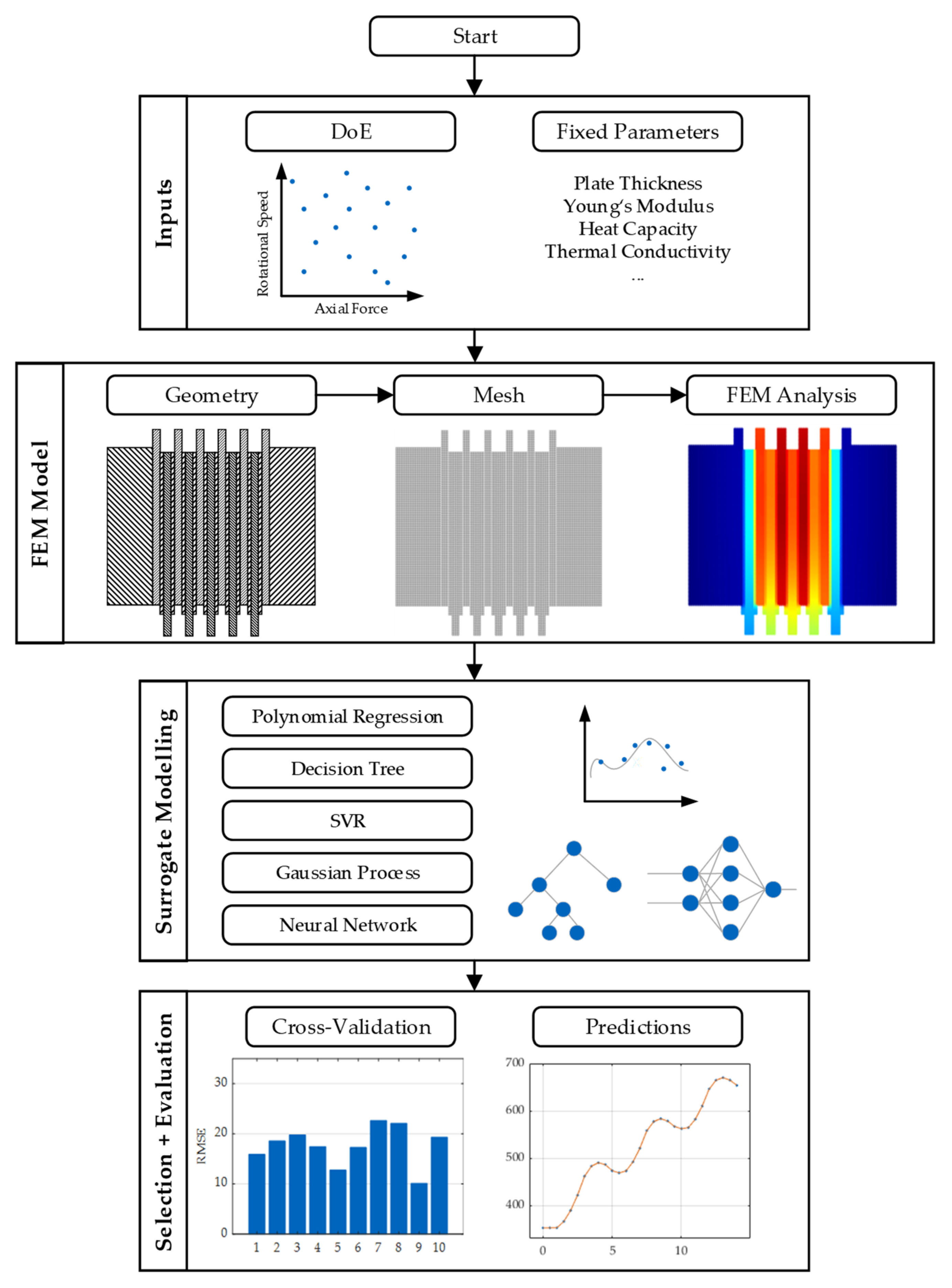
This study deals with the creation of surrogate models of a thermoelastic finite element simulation. The overall procedure is illustrated in Figure 1. The procedure can be roughly subdivided into four stages. The first step consists of the generation of the required data from the FE model. These are then processed in order to facilitate the creation of the surrogate models. In the last step, the generated models are subjected to a parameter study to investigate the influence of the sample size on the model performance. The individual steps are described in more detail in the following sections.

2.1. FE-Model and Use Cases

The model developed and presented by Schneider et al. [20] was used as a basis for the research presented in this paper. The model is a parameterizable two-dimensional model of a multi-plate clutch in transient operation. The geometry of the illustrated clutch and the corresponding FE model are shown in Figure 2. The clutch pack consists of 6 steel plates and 5 carrier plates with linings on both sides and comprises 10 friction surfaces. Furthermore, the reaction and pressure plates are placed on the left and right.

The simulation model can be divided into two distinct parts. In the first part, the mechanical aspects of the simulation are considered. The pressures and strains due to mechanical and thermal loads within the components are calculated based on the current axial force, speed and temperature distribution. The thermal aspects of the simulation are considered in the second part. Based on the pressure distribution calculated in the first part, the heat flows generated at the friction surfaces can be calculated. These are applied as loads for the thermal simulation. Subsequently, the transient thermal simulation is performed, and it provides the temperature distribution at the coupling as a result. After the two simulation stages have been carried out, the operating conditions of the clutch (pressure and temperature distribution) are updated. This procedure represents 1 time step. This procedure is performed for the defined number of time steps, each with the updated operating conditions as the initial condition. The complete process flow can be seen in Figure A1 in Appendix A. A time step size of 0.5 s and an element size of 0.0002 m were adopted. The simulation was carried out for 28 steps (14 s). The initial temperature of the clutch is 80 °C or 353.15 K.

Figure 3 is a comparison of the experimentally determined data and the results of the FE simulation. The experimental temperatures were measured at a point inside the third steel plate. These were compared with the associated temperature determined by the simulation. Figure 3a shows that the FE simulation reproduced the temporal temperature variation with good precision. Figure 3b shows the measured and simulated temperature increases, along with the identity line. There was a strong correlation between the measured and the simulated data.

The model enables the variation of a large number of parameters that influence the experienced load, the geometry of the clutch system and the material data of the installed components. Given that the study focused on creating a model suitable for operation, parameters that may vary during operation, such as load (axial force and speed) and lining thickness (due to wear of the lining), were considered. Other design and material parameters, such as the thickness of the steel plate or the Young’s modulus, do not change during operation and were therefore not considered in the modeling. Two different use cases were considered and are presented in

Table 1. Description of the two use cases with the corresponding examined parameters.

Use Case	Description	Varied Parameters
1	Load	Axial force Rotational speed
2	Load + lining wear	Axial force Rotational speed Lining thickness

.

Use Case 1 only covered operations under varying loads. The axial force and the speed were varied. The profiles of the axial force applied and the differential rotational speed are shown by way of example in Figure 4. In this research, the clutch is analyzed in transient slip conditions. The axial force is applied and the differential force is increased and then reduced to zero again. In Use Case 2, the wear and tear of the lining during operation was taken into account in addition to the load parameters.

2.2. Dataset Generation

The data employed to generate the surrogate models originate from the FE model described above. For each combination of input parameters, the simulation outputs the temperature distribution of the clutch at each time step. Since the maximum temperature is of interest concerning the damage mechanisms, the maximum value from the temperature distribution at each time step was selected. An illustrative temperature distribution with the corresponding maximum temperature is shown in Figure 5.

For the generation of the datasets, 200 simulations were run per use case. A Latin hypercube sampling was employed for the sampling of the parameter combinations. The lower and upper bounds of the individual parameters are shown in

Table 2. Boundaries of the varied input parameters.

Parameter	Lower Bound	Upper Bound
Axial force in kN	9.292	37.168
Rotational speed in rpm	80	140
Lining thickness in mm	0.2	0.8

. Each simulation yields a tuple $(p_i, T_i$), where $p_i\in {ℝ}^m$ is an $m$-dimensional vector representing the $m$ varied parameters of the respective use case ($m$ = 2 for Use Case 1 and $m$ = 3 for Use Case 2) and $T_i\in {ℝ}^{29}$ is a vector with the maximum temperature $T_{max}$ at the each of the 29 timesteps (see

Table 3. Input and output variables of the respective use cases.

Simulation	Use Case 1	Use Case 2
Input variables	Axial force Rotational speed Time	Axial force Rotational force Lining thickness Time
Output variable	Tmax	Tmax

).

Since there was a large difference in the magnitude of the individual input data, the latter were scaled to obey a standard normal distribution after scaling. Furthermore, no outliers within the data were expected given the FE simulation’s deterministic nature. The complete data set consisting of 200 simulations (5900 data points) is divided into a training set and a test set. The test set comprised the data from 25 simulations (725 data points), while the remaining data points were assigned to the training sets. The goal of this split was to evaluate the quality of the predictions of the trained models on cases not yet seen. Different subsets of the training sets of different sizes were created to investigate the influence of the size of the data set and the required number of simulations for adequate surrogate model generation. Training sets comprising 25, 50, 75, 100, 125, 150, and 175 simulations were examined. The data set with 100 simulations (2900 data points) was used as a baseline for this research.

2.3. Model Development

Five different machine learning methods are investigated to construct the surrogate model. These are explained in greater depth below. Unless otherwise noted, more information on each algorithm can be found in the work by Murphy [21].

• Polynomial Regression (PR): Polynomial regression is a subclass of linear regression, in which a basis function expansion is performed with polynomial functions [8,21]. The use of higher order polynomial functions enables non-linear relationships to be modeled. The PR model is given by:

  $$f\left(x\right)=w^T\varphi \left(x\right)$$

  (1)

  with

  $$\varphi \left(x\right)=\left[1, x, x^2,\dots , x^d\right]$$

  (2)

  where $w$ is the vector with the weight factors and $d$ is the selected polynomial order. Although PR models are very popular due to their simple calculation and the option of deriving conclusions about the influences of the individual input parameters [8], these models suffer from the disadvantage of being prone to overfitting for high polynomial degrees [21].
• Decision Tree (DT): Decision trees are methods that divide the input space into several areas. These subdivisions take place along the individual axes of the input space by means of the CART algorithm and can be represented by means of a tree. The mean value $w_i$ is calculated for each of the regions $R_i$ created after the subdivision. The output value of the model is given by the following expression:

  $$f\left(x\right)={\displaystyle \sum }_{i=1}^n{w}_i\mathbb{I}\left(x\in R_i\right)$$

  (3)
• Support Vector Regression (SVR): Support vector regression is a parametric model that uses kernels and considers only a portion of the training dataset to generate predictions. SVR models for a predefined kernel $\kappa$ can generically be defined by the following equation:

  $$f\left(x\right)=w_0+{\displaystyle \sum }_{i=1}^n{w}_i\kappa \left(x_i,x\right)$$

  (4)

  where $w$ are the parameters to be calculated.

A combination of ${\ell }_2$ regularization and epsilon insensitive loss function is used as the cost function. With the use of the epsilon insensitive loss function, all data points located within a band of width epsilon are not penalized. As a result, the model can be obtained by solving the constrained optimization problem given by Equation (5) [21]:

$$\begin{gathered} \min \frac{1}{2}{\left|w\right|}^2+C{\displaystyle \sum }_{i=1}^n\left({\xi }_i^{+}-{\xi }_i^{-}\right) \\ s.t. \{\begin{array}{c}{y}_i-f\left(x_i\right)\le ϵ+{\xi }_i^{+}\\ f\left(x_i\right)-y_i\le ϵ+{\xi }_i^{-}\\ {\xi }_i^{+},{\xi }_i^{-}\ge 0 \end{array} \end{gathered}$$

(5)

where ${\xi }_i^{+}$ and ${\xi }_i^{-}$ are introduced as slack variables and indicate the extent to which a data point lies outside the $ϵ$-band. The hyperparameter $C$ regulates the tradeoff between the flatness of the model and the degree to which deviations larger than $ϵ$ are tolerated. One of the drawbacks of these methods is the high computational cost of constructing the models. Interested readers can refer to Smola and Schölkpf [22] for more information on SVR.

4.

Gaussian Process (GP): Gaussian processes are non-parametric methods having the inference of distributions over functions as a basic principle [21]. If the data is noise-free, then GPs have the capability to interpolate the data points exactly. This is advantageous when creating surrogate models of deterministic FE models [23]. For the measured values $f$ at the sample points $X$ and the values $f_{*}$ being predicted at the points $X_{*}$, the joint probability distribution is given by:

$$\left(\begin{array}{c}f\\ f_{*}\end{array}\right)~\mathcal{N}\left(\left(\begin{array}{c}\mu \\ {\mu }_{*}\end{array}\right), \left(\begin{array}{cc}K& K_{*}\\ K_{*}^T& K_{**}\end{array}\right)\right)$$

(6)

with

$$K=\kappa \left(X,X\right),K_{*}=\kappa \left(X,X_{*}\right),K_{**}=\kappa \left(X_{*},X_{*}\right)$$

(7)

where $\kappa$ is the selected kernel or covariance function. The posterior probability distribution $p$ of the functions can be used to determine the predictions on the selected points $X_{*}$ and is given by:

$$p\left(f_{*}|X_{*}, X,f\right)=\mathcal{N}(f_{*}|{\mu }_{*}, {\mathsf{\Sigma }}_{*})$$

(8)

$${\mu }_{*}=\mu \left(X_{*}\right)+K_{*}^T{K}^{-1}\left(f-\mu \left(X\right)\right)$$

(9)

$${\mathsf{\Sigma }}_{*}=K_{**}-K_{*}^T{K}^{-1}{K}_{*}$$

(10)

For further background on Gaussian processes, the reader is referred to the work of Rasmussen and Williams [24].

5.

Backpropagation Neural Network (BPNN): Neural networks are a set of models based on the structure and function of biological neurons and consist of a number of layered and interconnected units (neurons) [8]. The output $h$ of a neuron consists of a linear combination of the inputs, which is then subjected to a nonlinear activation function:

$$h_{W,b}=\varphi \left(XW+b\right)$$

(11)

where $X$ is the matrix with the layer inputs, $W$ is the weight matrix, $b$ is the bias vector and $\varphi$ is the selected activation function. Given a network architecture, the network can be trained using a backpropagation algorithm to solve a specific problem [8,25].

Each algorithm was subjected to hyperparameter optimization. All of the hyperparameters examined are listed in

Table 4. Hyperparameters.

Model	Hyperparameter	Values
Polynomial Regression	Degree	[1, 10]
Decision Tree	Depth	{inf, 5, 10, 15, 20}
	Criterion	{‘squared_error’, ‘friedman’, ‘poisson’}
Support Vector Regression	Kernel	Linear, poly, RBF
	C	1, 10, 100, 1000
	Epsilon	1 × 10 −4, 1 × 10 −3, 1 × 10 −2
Gaussian Process	Kernel	DotProduct, RationalQuadratic, RBF
	Alpha	[1 × 10 −5, 1 × 10 −2]
Backpropagation Neural Networks	Number of hidden layers Number of neurons per layers Learning rate	[1, 10] [1, 50] [1 × 10 −5, 1 × 10 −1]

. All of the models were implemented in Python. The algorithms and implementations available in the Scikit-Learn package [26] were used for the PR, DT, SVR, and the GP. The Tensorflow package [27] with the Keras API was also employed for the BPNN.

2.4. Model Evaluation

In order to investigate the generalization capabilities of the models and to ensure independence of the results from the randomly selected dataset, the models were subjected to a nested cross-validation procedure. The process consists of two nested loops. The inner loop is dedicated to determining the optimal hyperparameters for a given fold of the data. For this purpose, a grid search (PR, DT, SVR, GP) or a randomized search (BPNN) with 3-fold cross-validation was performed. The generalization capabilities of the best model determined in the inner loop are examined in the outer loop (see Figure 6). To further investigate the performance of the models, the models were further evaluated using the test set.

The mean squared error (MSE), the root mean squared error (RMSE) and the mean absolute percentage error (MAPE) were employed as metrics to measure the quality of the models. These can be calculated according to Equations (12)–(14):

$$MSE=\frac{1}{n}{\displaystyle \sum }_{i=1}^n{\left(y_i-{\widehat{y}}_i\right)}^2$$

(12)

$$RMSE=\sqrt{MSE}$$

(13)

$$MAPE=\frac{1}{n}{\displaystyle \sum }_{i=1}^n\frac{\left|y_i-{\widehat{y}}_i\right|}{\left|y_i\right|}$$

(14)

where $y_i$ are the true values, ${\widehat{y}}_i$ are the predicted values and $n$ is the number of samples.

3. Results

The following section presents the results of the investigations for both use cases. The first part presents the performance of each model during the training process. The FE simulations were performed on a workstation with 96GB (12 × 8 GB) RAM, a NVIDIA Quadro P2000 5 GB (4) DP GFX GPU, and two Intel Xeon 6154 3.0 processors. The development of the surrogate models and the computation of the inference times were performed on a machine with 16 GB RAM and an Intel i7 processor.

3.1. Use Case 1—Axial Force + Rotational Speed

The RMSE scores of the 10-fold cross-validation for the polynomial regression, decision tree, support vector regression, and Gaussian process are shown in Figure 7. For the PR model, except for the third fold, low RMSE values with a mean of 8.12 were evident without considerable variance. In the case of the decision tree model, an average RMSE score of 17.60 was obtained, with the values of the individual folds ranging from 10 to 23. Similarly, in the case of the SVR, all scores were above 20, and an average RMSE score of 25.97 was achieved. The RMSE values for the cross-validation of the Gaussian process model exhibited the lowest mean value, at 7.41. However, the scores of the individual folds demonstrated a strong variance between themselves. As was the case with the PR, the third fold yielded an RMSE score of over 20, while the first fold, for example, had an RMSE score of only 1.93.

Figure 8 presents the training history for the BPNN. The training was performed for 10,000 epochs. Early stopping was used as a threshold to stop the training if the validation loss did not improve for 100 epochs. The learning rate was adjusted during training so that if the validation loss reached a plateau and did not improve for 50 epochs, the learning rate was reduced by half. The plotted curve shows that the training process converged to a RMSE of 3.45 after approximately 1200 epochs. The RMSE for the validation set amounted to 3.61, which indicates that no overfitting occurred.

Prediction on the test data (725 data points) set were performed to verify further the ability of the models to generate accurate predictions based on unused data. The RMSE and the R-squared values for each model for the test dataset are listed in

Table 5. Results of the models on the test set for Use Case 1.

	PR	DT	SVR	GP	BPNN	FE Model
RMSE	9.535	17.564	28.22	6.772	4.290	-
MAPE	1.36%	2.15%	3.69%	0.74%	0.51%	-
Training time in s	<1	<1	$~15$	$~110$	$~350$	-
Inference time in s	0.018	0.007	0.233	0.277	0.948	$~1100$

. The computation time required for the inference is provided as well.

As during the training procedure, the BPNN achieved the best RMSE score of 4.29, followed by the GP model, with 6.772. The PR model also achieved a comparatively low RMSE of 9.535, while both the DT and SVR models performed the poorest, with higher RMSE scores of 17.564 and 28.22, respectively. All models yielded MAPE values between 0.51% (BPNN) and 3.69% (PR). The order of performance of the models was analogous to the RMSE values. Concerning the required computing time, the individual algorithms differed slightly. Given its higher complexity, the BPNN required the highest computing time. In this sense, PR and DT were the most efficient algorithms with very short computation times of less than 0.1 s. All inference times, however, fell below the 1.0 s range, but were virtually negligible compared to the more than 1000 s required for the FE simulation.

To further illustrate the results and explore the application of the models, the predictions for a selected slip cycle are shown in Figure 9. Overall, all models except the SVR model provided good predictions for the selected circuit. In this particular instance, the GP model almost reproduced the data, whereas the PR and the BPNN exhibited only weak deviations at certain points. In the case of DT, the shape of the curve was correctly mapped, but a weak general shift of the curve to higher temperatures was evident. The model thus provided a higher maximum temperature than the simulated values. Noticeable in the case of the SVR model is that the model has difficulty reproducing the oscillations in temperature. As a result, this model exhibited the worst performance.

To investigate the influence of the volume of data, Figure 10 illustrates the obtained RMSE for each model as a function of the number of simulations used. Overall, it became evident that for all algorithms an increase in the amount of data also led to an improvement in performance (even if only a slight one in some cases). In the case of the SVR, a slight improvement was seen up to 50 simulations, whereas there was practically no variation in the results thereafter. In the case of the PR model, a strong improvement was present up to 90 simulations. For both DT and BPNN, the performance of the models improved with larger datasets, but the trend was noisy. In the case of the GP model, a very smooth curve was evident where performance improved continuously with higher data volumes.

3.2. Use Case 2—Axial Force + Rotational Speed + Lining Thickness

The results of the 10-fold cross-validation for Use Case 2 are shown in Figure 11. The PR and SVR showed very similar behavior and performance. The RMSE values of the individual folds for both models were similar, and the average RMSE values amounted to 26.67 and 27.59, respectively. The DT performed better, with an average RMSE score of 20.20. However, there was a large variance between the individual folds values, ranging from 13 to 27. This higher variance was also evident in the case of the Gaussian process, in which the values varied between 11 and 26. However, among these four models, the GP achieved the best performance during cross-validation with an average RMSE score of 18.03.

Figure 12 presents the training history of the BPNN for Use Case 2. The training was performed with the same settings as in Use Case 1. As in the first use case, the RMSE for both the training set and the validation set converged. After about 850 epochs, an RMSE of 6.94 was achieved for the training set. The validation loss (RMSE) amounted to 6.25. As was similar to Use Case 1, the BPNN did not demonstrate any overfitting issue.

Table 6. Results of the models on the test set for Use Case 2.

	PR	DT	SVR	GP	BPNN	FE Model
RMSE	24.614	19.706	24.756	14.434	6.312	-
MAPE	4.02%	2.18%	3.65%	2.20%	0.99%	-
Training time in s	<1	<1	$~15$	$~120$	$~400$	-
Inference time in s	0.026	0.001	0.260	0.306	0.311	$~1100$

shows the performance of the created methods on the test set. The performance of the models follows the order in cross-validation on the training dataset. Both polynomial regression and SVR showed the worst results, with RMSE values of approximately 24. The decision tree model performed slightly better, with an RMSE score of 19.71. Similar to the first use case, the Gaussian process and backpropagation neural network performed best, with RMSE values of 14.43 and 6.31, respectively. Whereas the SVR had the worst RMSE value, a better MAPE value than that of the PR was achieved. Although the GP performed better than the DT in terms of RMSE, both achieved similar MAPE values of about 2.2%. In terms of both RMSE and MAPE, the BPNN achieved the best performance.

In the example of individual slip cycles in Figure 13, the same behavior was seen for the PR and the SVR as for the SVR in Use Case 1. The general increase in temperature was modeled, but the temperature fluctuations were not captured. This effect was also present in a weakened form in the case of the GP. The DT modeled properly models the oscillatory temperature rises, but exhibited a deviation in the range between 5 and 10 s. As in the first use case, the predicted and true temperatures matched best in the case of the BPNN.

Figure 14 illustrates the model’s performance dependence as a function of the amount of data for Use Case 2. For the PR model it was evident that almost zero correlation was present. Only small fluctuations in the range between RMSE scores of 25 and 30 took place. The SVR modeled performs worse than the PR model for up to 50 simulations. Above 50 simulations, the performance of the two models was very similar. The decision tree model showed the worst performance at a low number of simulations but improved continuously when increasing the amount of data. Starting with about 100 simulations, an RMSE score of about 20 was achieved. Larger amounts of data did not exhibit any further significant improvement. As with Use Case 1, the Gaussian process showed a high dependence on the amount of data. A steady improvement of the results was observed with an increase in the data volume. The best performance was consistently achieved for all data volumes by the BPNN models. Better results than those for the PR and SVR were already achieved with only 10 simulations. From about 60 simulations onwards, there was a further significant improvement in performance. Starting from 100 simulations, a further improvement took place, but only to a small extent.

4. Discussion

Considering the magnitude of the RMSE values (between 4.29 and 28.22) in relation to the magnitude of the output variable (temperature ranging between 350 K and 1000 K), none of the five models considered turned out to be completely unsuitable regarding temperature predictions based on the axial force and the rotational speed. This outcome was also confirmed by the MAPE scores. Average absolute deviations of no more than 4.02% were achieved in all models in both use cases. Nevertheless, both the GP and BPNN stood out as the best alternatives for the surrogate models. The disadvantages of these two models was a significantly higher level of complexity than the PR, DT, and SVR, as well as the greater training time. Furthermore, all the models met the requirement of providing nearly real-time temperature predictions during operation. The inference times obtained were negligible compared to the simulation time and the duration of the switching process. The PR model, which is characterized by its simplicity, also achieved acceptable results in the first use case. In the second use case, which also considered the variation of the lining thickness during operation, the GP and the BPNN provided the best results. The PR models, which competed with the two best models (GP and BPNN) in Use Case 1, demonstrated significantly worse performance in this case.

Suppose not only the RMSE and MAPE scores, which indicate the average performance of the models, are taken into account, but individual slip cycles are analyzed as well. In that case, the SVR can be directly discarded as a good surrogate model. In both use cases, the SVR did not manage to reproduce the oscillations due to the three slip cycles in the temperature profile and only mapped the basic increase in temperature. Regarding Use Case 2, all but the DT and BPNN models exhibited the behavior of the SVR model in the first use case and they demonstrated weaknesses in replicating the fluctuations of the temperatures. It is also important to mention that Figure 9 and Figure 13 show only individual slip cycles as examples and that these results cannot be applied to all other slip cycles.

Regarding the research on the influence of data volume, both use cases showed that an increase in data volume fundamentally leads to improved performance. The range between 80 and 100 simulations can be considered preferable. In the two best models (GP and BPNN) an acceptable performance was reached within this range, with still manageable quantities of data to be generated. Larger data volumes achieved better results, but the improvement was not substantial.

In future work, we plan to extend the models to include more variables. For instance, the maximum temperature can be predicted in addition to the temperature of the material at any given x and y coordinates. Other geometry (steel plate thickness) and material parameters (Young’s modulus, heat capacity, etc.) or initial temperature distribution and oil temperature can also be taken into account. Based on these extended surrogate models, a sensitivity analysis can also be performed in order to further investigate the influences of the individual parameters on temperature behavior. Furthermore, other approaches such as physics-informed neural networks can be considered, which utilize not only the data, but also the existing physical knowledge about the domain to generate the models.

5. Conclusions

This paper examines the potential of constructing surrogate models based on machine learning methods for a two-dimensional thermo-mechanical finite element model of a multi-plate clutch. Based on the existing FE model, datasets of different sizes were generated and five machine learning algorithms were investigated: polynomial regression, decision tree, support vector regression, Gaussian process and backpropagation neural networks. The Gaussian process and the backpropagation neural networks emerged as the best models in both use cases. Polynomial regression shows good results in the first use case (axial force and speed as inputs) but underperformed when the lining thickness was additionally varied and considered as an input. Regarding the amount of data required, an improvement in performance for both GP and BPNN took place when the amount of data was increased. Acceptable results were achieved starting at about 60 FE simulations. In the context of the application, it was shown that ML-based surrogate models are able to adequately reproduce the thermo-mechanical behavior of the clutch system during operation.

References

- Groetsch, D.; Stockinger, U.; Schneider, T.; Reiner, F.; Voelkel, K.; Pflaum, H.; Stahl, K. Experimental investigations of spontaneous damage to wet multi-plate clutches with carbon friction linings. Forsch. Ing. 2021, 85, 1043–1052. [Google Scholar] [CrossRef]
- Stockinger, U.; Schneider, T.; Pflaum, H.; Stahl, K. Single vs. multi-cone synchronizers with carbon friction lining—A comparison of load limits and deterioration behavior. Forsch. Ing. 2020, 84, 245–253. [Google Scholar] [CrossRef]
- Schneider, T.; Bedrikow, A.B.; Völkel, K.; Pflaum, H.; Stahl, K. Comparison of Various Wet-Running Multi-Plate Clutches with Paper Friction Lining with Regard to Spontaneous Damage Behavior. Tribol. Ind. 2021, 43, 40–56. [Google Scholar] [CrossRef]
- Schneider, T.; Beiderwellen Bedrikow, A.; Völkel, K.; Pflaum, H. Load Capacity Comparison of Different Wet MultiPlate Clutches with Sinter Friction Lining with Regard to Spontaneous Damage Behavior. Tribol. Ind. 2022, 44, 394–406. [Google Scholar] [CrossRef]
- Marklund, P.; Larsson, R.; Lundström, T.S. Permeability of Sinter Bronze Friction Material for Wet Clutches. Tribol. Trans. 2008, 51, 303–309. [Google Scholar] [CrossRef]
- Schneider, T.; Zilkens, A.; Voelkel, K.; Pflaum, H.; Stahl, K. Failure Modes of Spontaneous Damage of Wet-Running Multi-Plate Clutches with Carbon Friction Linings. Tribol. Trans. 2022, 65, 813–826. [Google Scholar] [CrossRef]
- Schneider, T.; Völkel, K.; Pflaum, H.; Stahl, K. Einfluss von Vorschädigung auf das Reibungsverhalten nasslaufender Lamellenkupplungen im Dauerschaltbetrieb. Forsch. Ing. 2021, 85, 859–870. [Google Scholar] [CrossRef]
- Kudela, J.; Matousek, R. Recent advances and applications of surrogate models for finite element method computations: A review. Soft Comput. 2022, 1–25. [Google Scholar] [CrossRef]
- Vurtur Badarinath, P.; Chierichetti, M.; Davoudi Kakhki, F. A Machine Learning Approach as a Surrogate for a Finite Element Analysis: Status of Research and Application to One Dimensional Systems. Sensors 2021, 21, 1654. [Google Scholar] [CrossRef]
- Hoffer, J.G.; Geiger, B.C.; Ofner, P.; Kern, R. Mesh-Free Surrogate Models for Structural Mechanic FEM Simulation: A Comparative Study of Approaches. Appl. Sci. 2021, 11, 9411. [Google Scholar] [CrossRef]
- Roberts, S.M.; Kusiak, J.; Liu, Y.L.; Forcellese, A.; Withers, P.J. Prediction of damage evolution in forged aluminium metal matrix composites using a neural network approach. J. Mater. Process. Technol. 1998, 80–81, 507–512. [Google Scholar] [CrossRef]
- D’Addona, D.M.; Antonelli, D. Neural Network Multiobjective Optimization of Hot Forging. Procedia CIRP 2018, 67, 498–503. [Google Scholar] [CrossRef]
- Chan, W.L.; Fu, M.W.; Lu, J. An integrated FEM and ANN methodology for metal-formed product design. Eng. Appl. Artif. Intell. 2008, 21, 1170–1181. [Google Scholar] [CrossRef]
- Liang, L.; Liu, M.; Martin, C.; Sun, W. A deep learning approach to estimate stress distribution: A fast and accurate surrogate of finite-element analysis. J. R. Soc. Interface 2018, 15, 20170844. [Google Scholar] [CrossRef] [Green Version]
- Madani, A.; Bakhaty, A.; Kim, J.; Mubarak, Y.; Mofrad, M. Bridging finite element and machine learning modeling: Stress prediction of arterial walls in atherosclerosis. J. Biomech. Eng. 2019, 141, 084502. [Google Scholar] [CrossRef]
- Lorente, D.; Martínez-Martínez, F.; Rupérez, M.J.; Lago, M.A.; Martínez-Sober, M.; Escandell-Montero, P.; Martínez-Martínez, J.M.; Martínez-Sanchis, S.; Serrano-López, A.J.; Monserrat, C.; et al. A framework for modelling the biomechanical behaviour of the human liver during breathing in real time using machine learning. Expert Syst. Appl. 2017, 71, 342–357. [Google Scholar] [CrossRef] [Green Version]
- Martínez-Martínez, F.; Rupérez-Moreno, M.J.; Martínez-Sober, M.; Solves-Llorens, J.A.; Lorente, D.; Serrano-López, A.J.; Martínez-Sanchis, S.; Monserrat, C.; Martín-Guerrero, J.D. A finite element-based machine learning approach for modeling the mechanical behavior of the breast tissues under compression in real-time. Comput. Biol. Med. 2017, 90, 116–124. [Google Scholar] [CrossRef]
- Mozaffar, M.; Paul, A.; Al-Bahrani, R.; Wolff, S.; Choudhary, A.; Agrawal, A.; Ehmann, K.; Cao, J. Data-driven prediction of the high-dimensional thermal history in directed energy deposition processes via recurrent neural networks. Manuf. Lett. 2018, 18, 35–39. [Google Scholar] [CrossRef]
- Anandan Kumar, H.; Kumaraguru, S.; Paul, C.P.; Bindra, K.S. Faster temperature prediction in the powder bed fusion process through the development of a surrogate model. Opt. Laser Technol. 2021, 141, 107122. [Google Scholar] [CrossRef]
- Schneider, T.; Dietsch, M.; Voelkel, K.; Pflaum, H.; Stahl, K. Analysis of the Thermo-Mechanical Behavior of a Multi-Plate Clutch during Transient Operating Conditions Using the FE Method. Lubricants 2022, 10, 76. [Google Scholar] [CrossRef]
- Murphy, K. Machine Learning—A Probabilistic Perspective; MIT Press: Cambridge, MA, USA, 2014; ISBN 978-0262018029. [Google Scholar]
- Smola, A.J.; Schölkpf, B. A Tutorial on Support Vector Regression. 2003. Available online: https://alex.smola.org/papers/2003/SmoSch03b.pdf (accessed on 18 July 2022).
- Jiang, P.; Zhou, Q.; Shao, X. Surrogate Model-Based Engineering Design and Optimization; Springer: Singapore, 2020; ISBN 978-981-15-0730-4. [Google Scholar]
- Rasmussen, C.E.; Williams, C.K.I. Gaussian Processes for Machine Learning, 3rd ed.; MIT Press: Cambridge, MA, USA, 2008; ISBN 026218253X. [Google Scholar]
- LeCun, Y.; Bengio, Y.; Hinton, G. Deep learning. Nature 2015, 521, 436–444. [Google Scholar] [CrossRef]
- Pedregosa, F.; Varoquaux, G.; Gramfort, A.; Michel, V.; Thirion, B.; Grisel, O.; Blondel, M.; Müller, A.; Nothman, J.; Louppe, G.; et al. Scikit-learn: Machine Learning in Python. J. Mach. Learn. Res. 2012, 12, 2825–2830. [Google Scholar] [CrossRef]
- Abadi, M.; Barham, P.; Chen, J.; Chen, Z.; Davis, A.; Dean, J.; Devin, M.; Ghemawat, S.; Irving, G.; Isard, M.; et al. TensorFlow: A System for Large-Scale Machine Learning. 2015. Available online: https://www.tensorflow.org/ (accessed on 7 July 2022).
Figure 1.
Graphical representation of the general procedure.
Figure 2.
(
a) Geometrical dimensions and mechanical boundary conditions [
20] and (
b) FE model of the multi-plate clutch [
20].
Figure 3.
a) Measurement recording of a slip cycle and comparison of the simulated temperature with the measured temperature [
b) Comparison between simulated and measured temperature increase for different loads represented by individual circles [
Figure 4.
Exemplary curve of the axial force and differential rotational speed [
Figure 5.
Temperature distribution of the clutch at (a) 0 s, (b) 14 s, (c) 28 s.
Figure 6.
Graphical representation of the nested cross-validation procedure.
Figure 7.
RMSE for 10-fold cross-validation of the PR, DT, SVR and GP models for Use Case 1.
Figure 8.
Training and validation loss of the BPNN during training for Use Case 1.
Figure 9.
Exemplary predictions by the individual models for a slip cycle for Use Case 1.
Figure 10.
RMSE scores for the test sets as a function of the data volume for Use Case 1.
Figure 11.
RMSE for 10-fold cross-validation of the PR, DT, SVR and GP models for Use Case 2.
Figure 12.
Training and validation loss of the BPNN during training for Use Case 2.
Figure 13.
Exemplary predictions by the individual models for a slip cycle for Use Case 2.
Figure 14.
RMSE scores for the test sets as a function of the data volume for Use Case 2.