Integrating the Opposition Nelder–Mead Algorithm into the Selection Phase of the Genetic Algorithm for Enhanced Optimization

Abstract

In this paper, we propose a novel methodology that combines the opposition Nelder–Mead algorithm and the selection phase of the genetic algorithm. This integration aims to enhance the performance of the overall algorithm. To evaluate the effectiveness of our methodology, we conducted a comprehensive comparative study involving 11 state-of-the-art algorithms renowned for their exceptional performance in the 2022 IEEE Congress on Evolutionary Computation (CEC 2022). Following rigorous analysis, which included a Friedman test and subsequent Dunn’s post hoc test, our algorithm demonstrated outstanding performance. In fact, our methodology exhibited equal or superior performance compared to the other algorithms in the majority of cases examined. These results highlight the effectiveness and competitiveness of our proposed approach, showcasing its potential to achieve state-of-the-art performance in solving optimization problems.

1. Introduction

Optimization is a fundamental concept in various fields, including mathematics, computer science, engineering, economics, and operations research. It involves finding the best possible solution to a problem within a given set of constraints. The goal of optimization is to maximize or minimize an objective function, which represents the measure of performance or utility [1].

In optimization, the objective is to find the optimal solution that achieves the highest possible value for a maximization problem or the lowest possible value for a minimization problem. The solution can be a single point in the search space or a set of values for multiple variables or parameters [2]. The process of optimization typically involves defining the problem, specifying the objective function and constraints, selecting an appropriate optimization algorithm or method, and iteratively refining the solution to converge toward the optimal outcome [3]. The optimization algorithm explores the search space, evaluating different candidate solutions and making adjustments based on specific rules or principles to improve the objective function value [4]. Typically, a constrained optimization problem can be mathematically formulated as follows: Minimize (or maximize) the objective function $f\left(\mathbf{x}\right)$ subject to a set of constraints $g_i\left(\mathbf{x}\right)\le 0$ and $h_j\left(\mathbf{x}\right)=0$, where $\mathbf{x}$ is the vector of decision variables with a dimension of D. Mathematically, it can be written as [2]:

Minimize:

$$f\left(\mathbf{x}\right)$$

(1)

Subject to:

$$g_i\left(\mathbf{x}\right)\le 0,i\in \{1,\dots ,M\}$$

(2)

$$h_j\left(\mathbf{x}\right)=0,j\in \{1,\dots ,N\}$$

(3)

$$\mathbf{x}=[x^{\left(1\right)},\dots ,x^{\left(D\right)}]\in [x_{min}^{\left(1\right)},x_{max}^{\left(1\right)}]\times \dots \times [x_{min}^{\left(D\right)},x_{max}^{\left(D\right)}]$$

(4)

Here, $f\left(\mathbf{x}\right)$ represents the objective function that needs to be minimized or maximized. The decision variables are represented by the vector $\mathbf{x}$, which can be a single variable or a set of variables with a dimension of D. The constraints are defined by the functions $g_i\left(\mathbf{x}\right)$ and $h_j\left(\mathbf{x}\right)$. The inequality constraints $g_i\left(\mathbf{x}\right)\le 0$ represent the conditions that must be satisfied, and the equality constraints $h_j\left(\mathbf{x}\right)=0$ represent the equality relationships in the problem. The index i ranges from 1 to M for inequality constraints, and the index j ranges from 1 to N for equality constraints. If the problem does not have inequality and equality constraints, it is called an unconstrained optimization problem [5]. The solution to the constrained optimization problem is a vector ${\mathbf{x}}^{*}$ that optimizes the objective function $f\left(\mathbf{x}\right)$ while satisfying all the constraints. The goal is to find the values of the decision variables ${\mathbf{x}}^{*}$ that minimize or maximize the objective function while satisfying the given constraints.

Various optimization techniques and algorithms can be employed to solve constrained optimization problems, such as gradient-based methods, linear programming, nonlinear programming, and evolutionary algorithms, depending on the problem’s characteristics and complexity. Optimization algorithms can be classified into several categories based on their approach and characteristics [6]. Four common categories are exact methods, approximation methods, metaheuristic methods, and derivative-based methods.

1.1. Exact Methods

Exact methods aim to find the optimal solution by exhaustively exploring the entire solution space. These algorithms guarantee that the solution obtained is the global optimum, but they may be computationally expensive and impractical for large-scale problems [7]. Some examples of exact methods include:

• Branch and bound: Divides the problem into smaller subproblems and prunes branches that are known to be suboptimal [8].
• Integer programming: Optimizes linear functions subject to linear equality and inequality constraints, with some or all variables restricted to integer values [9].
• Dynamic programming: Breaks down the problem into overlapping subproblems and solves them recursively, storing and reusing the intermediate results [10].

1.2. Approximation Methods

Approximation methods focus on finding a solution that is close to the optimal solution without guaranteeing optimality. These algorithms often provide good-quality solutions within a reasonable time frame and are suitable for large-scale problems where finding the global optimum is computationally infeasible. Some examples of approximation methods include:

• Greedy algorithms: Make locally optimal choices at each step to construct a solution incrementally [11].
• Randomized algorithms: Introduce randomness to explore the solution space and find near-optimal solutions [12].

1.3. Metaheuristic Methods

Metaheuristic methods are general-purpose optimization algorithms that guide the search for solutions by iteratively exploring the solution space. They are often inspired by natural phenomena or analogies and are applicable to a wide range of problems. Some popular metaheuristics methods include:

• Simulated annealing: Mimics the annealing process in metallurgy, allowing occasional uphill moves to escape local optima [13].
• Genetic algorithms: Inspired by the process of natural selection, genetic algorithms evolve a population of candidate solutions through selection, crossover, and mutation operations [14].
• Particle swarm optimization: Simulates the movement and interaction of a swarm of particles to find optimal solutions by iteratively updating their positions [15].
• Ant colony optimization: Mimics the foraging behavior of ants, where artificial ants deposit pheromones to guide the search for optimal paths or solutions [16].

1.4. Derivative-Based Methods

Derivative-based methods, also known as gradient-based methods, utilize information about the derivative of the objective function to guide the search for the optimum. These methods are effective when the objective function is differentiable. In other words, derivative-based methods are particularly useful in continuous optimization problems where the objective function is smooth and the derivatives can be efficiently computed. Some derivative-based optimization algorithms include:

• Gradient descent: Iteratively updates the solution in the direction of the steepest descent of the objective function [17].
• Newton’s method: Utilizes both the first and second derivatives of the objective function to approximate the optimum more efficiently [18].
• Quasi-Newton methods: Approximate the Hessian matrix (second derivatives) using a limited number of function and gradient evaluations to improve convergence speed [19].

It is important to note that this classification is not exhaustive, and there are other specialized optimization algorithms and techniques available for different types of problems. The choice of optimization algorithm depends on the problem characteristics, computational resources, and desired trade-offs between solution quality and computational efficiency [20]. In addition, optimization has diverse applications across various domains, such as engineering design, operations management, financial planning, scheduling, machine learning, and data analysis. It plays a crucial role in improving efficiency, resource allocation, decision making, and overall performance in a wide range of real-world problems. Here are some notable applications of optimization in our everyday lives:

• Transportation and routing: Optimization algorithms are used in transportation systems to optimize routes, schedules, and logistics. Whether it involves finding the shortest path for navigation apps, optimizing traffic signal timings, or planning public transportation routes, optimization helps minimize travel time, reduce congestion, and enhance overall transportation efficiency [21,22,23].
• Resource management: Optimization techniques are employed in diverse areas of resource management. For instance, energy companies optimize power generation and distribution to meet demand while minimizing costs. Water management systems optimize water distribution to ensure equitable supply and minimize wastage. Optimization is also applied in inventory management, supply-chain logistics, and workforce scheduling to optimize resource allocation and improve operational efficiency [24,25,26].
• Financial planning and investment: Optimization is widely used in financial planning and investment strategies. It helps investors optimize their portfolios by considering risk-return trade-offs. Optimization algorithms can determine the optimal allocation of funds across different assets or investment opportunities, aiming to maximize returns while managing risk within specified constraints [27,28].
• Production and manufacturing: Optimization is crucial in production and manufacturing processes to improve efficiency, reduce costs, and maximize output. Production scheduling optimization algorithms help determine the optimal sequence and timing of manufacturing operations. Additionally, optimization is utilized in capacity planning, facility layout design, and supply-chain optimization to streamline operations and minimize waste [29,30,31].
• Energy optimization: Energy optimization plays a significant role in promoting sustainable practices and reducing environmental impact. Optimization techniques are employed in energy-efficient buildings, where they control heating, ventilation, and air-conditioning systems to optimize energy consumption while maintaining comfort levels. Smart grid technologies also leverage optimization algorithms to optimize power generation, distribution, and consumption, facilitating energy conservation [32,33,34,35].
• Personal health and fitness: Optimization algorithms are increasingly being used in personal health and fitness applications. Fitness trackers and mobile apps employ optimization techniques to provide personalized exercise and diet plans, optimizing the balance between calorie intake and expenditure. These algorithms consider individual goals, preferences, and constraints to help users achieve desired health and fitness outcomes [36,37,38,39,40].
• Internet and e-commerce: Optimization algorithms are utilized in internet-based applications and e-commerce platforms to enhance the user experience and optimize various processes. From search engine algorithms that rank search results to recommendation systems that personalize product suggestions, optimization is employed to improve relevance, efficiency, and customer satisfaction [41,42,43].

These are just a few examples that highlight the wide range of applications where optimization algorithms and techniques are utilized to improve efficiency, decision making, and resource allocation in our daily lives. Optimization continues to drive advancements and contribute to enhancing various aspects of our modern society.

Hybrid metaheuristic algorithms represent a critical and evolving frontier in optimization research, addressing the inherent limitations of individual algorithms by harnessing the collective strengths of diverse optimization techniques. In a complex and dynamic problem landscape where no single algorithm universally excels, hybridization offers a compelling approach to achieving enhanced performance, increased robustness, and superior convergence rates. By fusing different algorithms, these hybrids can adapt to various problem characteristics, balance exploration and exploitation, and efficiently navigate high-dimensional solution spaces. As real-world challenges become more intricate, the ability of hybrid metaheuristics to provide innovative solutions is paramount, driving the progress of optimization methodologies across domains ranging from engineering and finance to artificial intelligence and beyond. Over the past few years, numerous hybrid algorithms have emerged in the literature, and we will examine a selection of these. The study outlined in [44] demonstrates two hybrid metaheuristic algorithms, specifically the genetic algorithm and the multiple population genetic algorithm, that are synergistically combined with variable neighborhood search to tackle some challenging NP-hard problems. The research highlighted in [45] portrays an innovative hybrid algorithm that merges genetic algorithms with the spotted hyena algorithm to effectively address the complexities of the production shop scheduling problem. The research work showcased in [46] describes an advanced hybrid metaheuristic approach for solving the traveling salesman problem with drones. This approach draws from two algorithms, namely the genetic algorithm and the ant colony optimization algorithm. The paper in [47] establishes an innovative approach known as the hybrid muddy soil fish optimization-based energy-aware routing scheme, designed to enhance the efficiency of routing in wireless sensor networks, facilitated by the Internet of Things. The research discussed in [48] introduces a novel metaheuristic approach, the hybrid brainstorm optimization algorithm, to effectively address the emergency relief routing problem. This innovative algorithm amalgamates concepts from the simulated annealing algorithm and the large neighborhood search algorithm into the foundation of the former, to significantly enhance its capacity to evade local optima and speed up the convergence process. The examination in [49] exposes a groundbreaking hybrid metaheuristic algorithm, termed the chaotic sand-cat swarm optimization, as a potent solution for intricate optimization problems that exhibit constraints. This algorithm seamlessly merges the attributes of the newly introduced technique with the innovative concept of chaos, promising enhanced performance in handling complex scenarios. The inquiry described in [50] introduces the hybridization of the particle swarm optimization with variable neighborhood search and simulated annealing to tackle permutation flow-shop scheduling problems. The findings detailed in [51] highlight an original hybrid algorithm integrating principles from the particle swarm optimization and puffer fish algorithms, aiming to accurately estimate parameters related to fuel cells. The study in [52] showcases the fusion of the brainstorm optimization algorithm with the chaotic accelerated particle swarm optimization algorithm. The purpose is to explore the potential enhancements that this amalgamated approach could offer over using the individual algorithms independently. The research elucidated in [53] presents an innovative hybrid learning moth search algorithm. This algorithm uniquely integrates two distinct learning mechanisms: global-best harmony search learning and Baldwinian learning. The objective is to effectively address the multidimensional knapsack problem, harnessing the benefits of these combined learning approaches.

The research described in this paper proposes a novel contribution by integrating the opposition Nelder–Mead algorithm into the selection phase of genetic algorithms to address the premature convergence problem and enhance exploration capabilities. This integration offers several significant advantages and advancements to the field of optimization and evolutionary computation, including:

• Prevention of premature convergence: Premature convergence is a common issue in genetic algorithms [54,55,56], where the algorithm converges to suboptimal solutions without adequately exploring the search space. By incorporating the opposition Nelder–Mead algorithm into the selection phase, our research provides a solution to this problem. The opposition Nelder–Mead algorithm, known for its effectiveness in local search and optimization [57], brings its exploratory power to the genetic algorithm. This integration ensures that the algorithm can avoid premature convergence by continuously exploring and exploiting promising regions of the search space.
• Enhanced exploration capabilities: The integration of the opposition Nelder–Mead algorithm into the selection phase enhances the exploration capabilities. Genetic algorithms traditionally rely on genetic operators such as crossover and mutation for exploration. However, these operators may not be sufficient to thoroughly explore complex search spaces [58]. By incorporating the opposition Nelder–Mead algorithm, which excels in local exploration, our methodology enhances the exploration capabilities of genetic algorithms. This integration enables a more comprehensive search of the search space, leading to the discovery of diverse and potentially better solutions.
• Improved convergence speed and solution quality: The integration of the opposition Nelder–Mead algorithm offers the potential for improved convergence speed and solution quality. The opposition Nelder–Mead algorithm is known for its efficiency in converging toward local optima. By utilizing this algorithm during the selection phase, our methodology aims to guide the genetic algorithm toward better solutions at a faster rate. This combination of global exploration from genetic algorithms and local optimization from the Nelder–Mead algorithm results in an algorithm that can converge faster and produce high-quality solutions. It is worth pointing out that the convergence speed in metaheuristics refers to the rate at which an algorithm approaches a solution of acceptable quality. It indicates how quickly an algorithm narrows down its search space and refines its solutions, ultimately aiming to find an optimal or near-optimal solution. A faster convergence speed implies that the algorithm reaches promising solutions in fewer iterations, whereas a slower convergence speed suggests that more iterations are needed to achieve comparable results. It is clear now that the integration of the iterative process of the Nelder–Mead algorithm into the iterative process of the genetic algorithm would improve its convergence speed.
• Practical applicability and generalizability: The proposed methodology holds practical applicability and generalizability. Genetic algorithms are widely used in various fields and domains for optimization problems. By addressing the premature convergence problem and enhancing exploration capabilities, our research contributes to the broader applicability and effectiveness of genetic algorithms in real-world scenarios. The integration can potentially be applied to a wide range of optimization problems, providing practitioners and researchers with a valuable tool to improve their optimization processes.

In summary, our research paper makes a significant contribution by integrating the opposition Nelder–Mead algorithm into the selection phase of genetic algorithms. This integration addresses the premature convergence problem, enhances exploration capabilities, improves convergence speed and solution quality, and offers practical applicability and generalizability. The proposed approach has the potential to advance the field of optimization and evolutionary computation, empowering practitioners and researchers with an effective tool for solving complex optimization problems.

This paper is organized into four sections: Section 2: Background; Section 3: Proposed Methodology; Section 4: Experimental Results and Discussion; and Section 5: Conclusions and Future Scope. Section 2 provides an overview of the relevant concepts used to establish the context for the research. Section 3 outlines the specific approach used to integrate the opposition Nelder–Mead algorithm into the selection phase of genetic algorithms and highlights its potential benefits. Section 4 presents the empirical evaluation of the proposed methodology, including the experimental setup, results, and analysis. Finally, Section 5 summarizes the key findings, discusses the implications of the research, and suggests potential future directions for further exploration.

2. Background

In this section, we broadly describe the underlying algorithms and techniques that are used to design our proposed methodology. Section 2.1 presents an overview of genetic algorithms as a powerful optimization technique. Genetic algorithms are population-based search algorithms that mimic the process of natural evolution to explore the solution space and find optimal solutions. Section 2.2 delves into the Nelder–Mead algorithm, which is a direct search method for optimization. It provides a detailed description of the algorithm’s basic operations, including reflection, expansion, contraction, and shrinkage, to iteratively converge toward the optimum. Lastly, Section 2.3 introduces the opposition-based learning technique, which is a novel concept that enhances optimization algorithms. It incorporates the use of opposite solutions to improve the exploration capabilities and convergence speed.

2.1. Genetic Algorithms

Genetic algorithms (GAs) [59] are a class of optimization algorithms inspired by the process of natural selection and genetics. They are widely used in various fields to solve complex optimization problems. This section provides an overview of the working principle of genetic algorithms, highlighting the key components and steps involved in their operation [60]:

• Initialization: The first step in a genetic algorithm is the initialization of a population. A population consists of a set of potential solutions to the optimization problem, known as individuals or chromosomes. Each individual represents a possible solution in the search space. The population is typically randomly generated or initialized based on prior knowledge of the problem domain.
• Fitness evaluation: Once the initial population is created, the fitness of each individual is evaluated. Fitness represents the quality or suitability of an individual solution with respect to the optimization objective. It is determined by an objective function that quantifies how well the individual performs. The objective function could be based on specific criteria, constraints, or a combination of both.
• Selection: The selection process simulates the concept of survival of the fittest, where individuals with higher fitness values have a higher probability of being selected for reproduction. Various selection methods can be employed, such as roulette-wheel selection, tournament selection, or rank-based selection [61]. The goal of selection is to create a mating pool consisting of individuals that are more likely to produce better offspring.
• Reproduction: Reproduction involves the creation of new individuals (offspring) through genetic operators, namely crossover and mutation. Crossover is the process of exchanging genetic information between two parent individuals, typically at specific points or positions within their representation. This exchange generates offspring that inherit characteristics from both parents. Mutation introduces random changes or modifications to the offspring’s genetic information, allowing for the exploration of new regions in the search space [62].
• Replacement: After the offspring are generated, a replacement strategy is applied to determine which individuals from the current population will be replaced by the newly created offspring. The replacement strategy can be based on various criteria, such as fitness-based replacement, elitism (preserving the best individuals), or a combination of both. This step ensures that the population evolves over time, favoring better solutions [62].
• Termination criteria: Genetic algorithms continue to iterate through the selection, reproduction, and replacement steps until a termination condition is met. Termination conditions can be based on a maximum number of generations, a specific fitness threshold, or a predefined computational budget. Once the termination condition is satisfied, the algorithm stops, and the best individual in the final population is considered the solution to the optimization problem.

Genetic algorithms offer a powerful approach to solving complex optimization problems. By mimicking the principles of natural selection and genetics, these algorithms iteratively evolve a population of potential solutions to converge toward an optimal or near-optimal solution. Understanding the working principle of genetic algorithms is crucial for effectively applying them to various domains and harnessing their potential in solving real-world optimization challenges. The advantages and disadvantages of GAs can vary depending on the problem domain and specific implementation. Some commonly cited advantages and disadvantages are described below [58,63].

2.1.1. Advantages of GAs

Some commonly cited advantages of GAs are:

• Global search capability: GAs are effective in exploring a large search space, allowing them to find global or near-global optimal solutions.
• Flexibility: GAs can handle various types of optimization problems, including continuous, discrete, and mixed-variable problems.
• Parallel processing: The parallel nature of GAs allows for distributed computing, enabling faster convergence and the ability to tackle computationally intensive problems.
• Robustness: GAs are often robust against noise or uncertainty in the objective function, making them suitable for real-world problems with noisy data or incomplete information.
• Solution diversity: GAs inherently maintain a diverse population, which helps avoid premature convergence and allows for the exploration of multiple regions of the search space.

2.1.2. Disadvantages of GAs

Some commonly cited disadvantages of GAs are:

• Computational complexity: GAs can be computationally expensive, especially for problems with large population sizes and complex fitness evaluations.
• Premature convergence: GAs may converge prematurely to a suboptimal solution if the selection pressure is too high or the genetic operators are not properly balanced.
• Parameter sensitivity: The performance of GAs can be sensitive to the choice of algorithmic parameters, such as population size, crossover and mutation rates, and termination criteria.
• Lack of problem-specific knowledge: GAs do not leverage problem-specific knowledge, and thus may require a significant number of function evaluations to converge to the optimal solution.
• Representation limitations: The choice of representation for the individuals can impact the performance of GAs, and certain problems may require specialized representations for effective optimization.

2.2. Nelder–Mead Algorithm

The Nelder–Mead algorithm [64], also known as the simplex method, is a popular optimization technique introduced by John Nelder and Roger Mead in 1965. It is a direct search method that does not require derivative information and is capable of handling both smooth and non-smooth objective functions.

The algorithm begins with an initial simplex, which is a geometric shape consisting of $n+1$ vertices in an n-dimensional space. Each vertex represents a potential solution to the optimization problem. The Nelder–Mead algorithm iteratively modifies and explores the simplex to search for the optimal solution.

At each iteration, the algorithm evaluates the objective function at each vertex of the simplex, identifying the best (lowest) function value (viz. $f\left({\mathbf{x}}_1\right)$), the worst (highest) function value (viz. $f({\mathbf{x}}_{n+1}$), and the second-worst function value (viz. $f\left({\mathbf{x}}_n\right))$) among the vertices. Based on these evaluations, the algorithm performs various operations to update the simplex:

• Reflection: The worst vertex is reflected through the centroid of the remaining n vertices. If the reflected vertex yields a better function value than the second-worst vertex but worse than the best vertex, it replaces the worst vertex. The reflection operation helps the algorithm explore the search space in the direction of the reflected vertex. The reflection phase can be summarized as follows:

  (a)

  Compute the reflection vertex ${\mathbf{x}}_r$ using Equation (5), where $\overline{\mathbf{x}}$ is the centroid of the n first best points (i.e., $\overline{\mathbf{x}}=\frac{1}{n}{\sum }_{i=1}^n{\mathbf{x}}_i$) and $\rho$ is the coefficient of reflection.

  $${\mathbf{x}}_r=(1+\rho )\overline{\mathbf{x}}+\rho {\mathbf{x}}_{n+1}$$

  (5)

  (b)

  If $f\left({\mathbf{x}}_1\right)\le f\left({\mathbf{x}}_r\right)<f\left({\mathbf{x}}_n\right)$, accept the reflected point ${\mathbf{x}}_r$ and terminate the iteration.

• Expansion: If the reflected vertex has a better function value than the best vertex, the algorithm performs an expansion operation. It calculates a new point by extrapolating beyond the reflected vertex and evaluates the function at this new point. If the new point is better than the reflected vertex, it replaces the worst vertex. The expansion operation allows the simplex to grow in the direction of the reflected vertex, potentially discovering better solutions. The expansion phase can be recapitulated as follows:

  (a)

  If $f\left({\mathbf{x}}_r\right)<f\left({\mathbf{x}}_1\right)$, compute the expansion vertex ${\mathbf{x}}_e$ using Equation (6), where $\chi$ is the coefficient of expansion.

  $${\mathbf{x}}_e=(1+\rho \chi )\overline{\mathbf{x}}-\rho \chi {\mathbf{x}}_{n+1}$$

  (6)

  (b)

  If $f\left({\mathbf{x}}_e\right)<f\left({\mathbf{x}}_r\right)$, accept ${\mathbf{x}}_e$ and terminate the iteration; otherwise, accept ${\mathbf{x}}_r$ and terminate the iteration.

• Contraction: If the reflected vertex does not improve the function value compared to the second-worst vertex, the algorithm performs a contraction operation. It calculates a new point by contracting toward the best vertex from the reflected vertex and evaluates the function at this new point. If the new point yields a better function value than the reflected vertex, it replaces the worst vertex. The contraction operation helps the algorithm converge toward the best vertex. The contraction phase can be described as follows:

  (a)

  If $f\left({\mathbf{x}}_n\right)\le f\left({\mathbf{x}}_r\right)<f\left({\mathbf{x}}_{n+1}\right)$, perform an outside contraction as follows:

  • Compute the outside contraction vertex ${\mathbf{x}}_{oc}$ using Equation (7), where $\gamma$ is the coefficient of contraction.

    $${\mathbf{x}}_{oc}=(1+\rho \gamma )\overline{\mathbf{x}}-\rho \gamma {\mathbf{x}}_{n+1}$$

    (7)
  • If $f\left({\mathbf{x}}_{oc}\right)<f\left({\mathbf{x}}_r\right)$, accept ${\mathbf{x}}_{oc}$ and terminate the iteration; otherwise, go to step 4.

  (b)

  If $f\left({\mathbf{x}}_r\right)\ge f\left({\mathbf{x}}_{n+1}\right)$, perform an inside contraction as follows:

  • Compute the inside contraction vertex ${\mathbf{x}}_{ic}$ using Equation (8), where $\gamma$ is the coefficient of contraction.

    $${\mathbf{x}}_{ic}=(1-\gamma )\overline{\mathbf{x}}+\gamma {\mathbf{x}}_{n+1}$$

    (8)
  • If $f\left({\mathbf{x}}_{ic}\right)<f\left({\mathbf{x}}_{n+1}\right)$, accept ${\mathbf{x}}_{ic}$ and terminate the iteration; otherwise, go to step 4.

• Shrinkage: If none of the above operations result in a better vertex, the algorithm performs a shrinkage operation. It shrinks the simplex toward the best vertex by updating each vertex, except the best vertex, to move closer to the best vertex by a certain fraction. This contraction of the simplex assists in refining the search around the current best solution. The shrinkage phase can be described as follows:

  (a)

  Update the vertices ${\mathbf{x}}_2,\dots ,{\mathbf{x}}_n,{\mathbf{x}}_{n+1}$ using Equation (9), where $\sigma$ is the coefficient of shrinkage.

  $${\mathbf{x}}_i={\mathbf{x}}_1+\sigma ({\mathbf{x}}_i-{\mathbf{x}}_1),i\in \{2,\dots ,n,n+1\}$$

  (9)

  (b)

  The new vertices calculated using Equation (9) are to be considered for the next iteration.

The iterations continue until certain convergence criteria are met, such as reaching a maximum number of iterations, achieving a small improvement in the function value, or obtaining a small change in the size of the simplex. The Nelder–Mead algorithm is widely used in various domains, including engineering, computer science, and mathematical optimization. It is particularly suitable for problems with non-smooth or non-convex objective functions. Although it does not guarantee finding the global optimum, it often converges to good local optima [57]. The Nelder–Mead algorithm is a derivative-free optimization algorithm commonly used to solve unconstrained optimization problems. Here are some advantages and disadvantages of the Nelder–Mead algorithm [64]:

2.2.1. Advantages of the Nelder–Mead Algorithm

Some advantages of the Nelder–Mead algorithm are:

• Simplicity: The Nelder–Mead algorithm is relatively easy to understand and implement compared to more complex optimization methods.
• No derivative information required: The algorithm does not rely on derivative information, making it suitable for optimizing functions that are not easily differentiable or when computing derivatives is computationally expensive.
• Convergence in certain cases: The Nelder–Mead algorithm can converge quickly for low-dimensional problems with smooth, convex objective functions.
• Robustness: It is relatively robust against noisy or imperfect function evaluations.

2.2.2. Disadvantages of the Nelder–Mead Algorithm

Some disadvantages of the Nelder–Mead algorithm are:

• Sensitivity to initial conditions: The performance of the Nelder–Mead algorithm is highly dependent on the initial simplex configuration. Poor initial setups may result in slow convergence or even failure to converge.
• Lack of global convergence guarantee: Unlike some other optimization algorithms, the Nelder–Mead algorithm does not have a guaranteed global convergence property. It can converge to a local minimum or even get trapped in non-optimal regions of the search space.
• Inefficiency in high-dimensional spaces: The performance of the Nelder–Mead algorithm deteriorates as the dimensionality of the problem increases, known as the “curse of dimensionality”. It may struggle to converge or require significantly more function evaluations in high-dimensional spaces.

2.3. Opposition-Based Learning

Opposition-based learning (OBL) [65] is a heuristic technique used in optimization algorithms to enhance the search process and improve the quality of solutions. It is inspired by the concept of opposition, which involves considering the opposite or contrasting characteristics of a given solution or search-space point. OBL introduces the notion of “opposition” to generate new candidate solutions by incorporating contrasting information. The general working principle of opposition-based learning involves the following steps [66]:

• Initialization: A population of candidate solutions is randomly generated or initialized within the search space.
• Evaluation: Each candidate solution is evaluated using an objective function to determine its fitness or quality.
• Opposition generation: Opposite solutions or individuals are generated for each candidate solution by incorporating contrasting information. This can be achieved in various ways, such as flipping binary values, negating numerical values, or applying specific transformation functions.
• Fitness evaluation for opposite solutions: The fitness of the opposite solutions is evaluated using the same objective function.
• Update and selection: The original candidate solutions and their opposite counterparts are compared based on their fitness values. The better solution between each pair (original and opposite) is selected and considered for the next iteration or generation.
• Repeat: Steps 2–5 are iteratively repeated until a termination condition is met, such as reaching a maximum number of iterations or achieving a desired level of convergence.

The use of opposition-based learning aims to promote exploration in the search space by considering contrasting information and potentially discovering new regions that may not be explored by traditional optimization techniques. By incorporating opposite solutions, OBL attempts to enhance the diversity and convergence properties of the optimization algorithm. Opposition-based learning has been applied in various optimization algorithms, including evolutionary algorithms, particle swarm optimization, and simulated annealing, among others. It has shown promising results in improving solution quality, convergence speed, and robustness in solving complex optimization problems [66]. The advantages and disadvantages of opposition-based learning can vary depending on the specific implementation and problem domain. Some commonly cited advantages and disadvantages are described below [66].

2.3.1. Advantages of OBL

Some advantages of OBL are:

• Improved solution quality: By considering contrasting information through opposite solutions, OBL can enhance the exploration of the search space, potentially leading to improved solution quality and diversity.
• Enhanced convergence properties: OBL can help optimization algorithms converge faster by introducing additional diversity and promoting the search in unexplored regions of the search space.
• Robustness: OBL has been shown to improve the robustness of optimization algorithms by reducing the risk of becoming trapped in local optimums.
• Widely applicable: OBL can be applied to various optimization algorithms and problem domains, making it a versatile approach to improving optimization performance.
• Simple implementation: OBL is relatively easy to implement, as it involves generating opposite solutions by incorporating contrasting information.

2.3.2. Disadvantages of OBL

Some disadvantages of OBL are:

• Increased computational complexity: The introduction of opposite solutions adds computational overhead, as it requires additional fitness evaluations and solution comparisons.
• Sensitivity to parameters: The performance of OBL can be sensitive to the choice of specific parameters, such as the method of generating opposite solutions or the selection criteria between original and opposite solutions.
• Limited exploration: Although OBL can enhance exploration, it may not always guarantee exploration of the entire search space, especially in complex and high-dimensional optimization problems.
• Lack of universally optimal opposite generation strategy: The choice of method for generating opposite solutions depends on the problem domain and algorithm used, and there is no universally optimal strategy applicable to all scenarios.

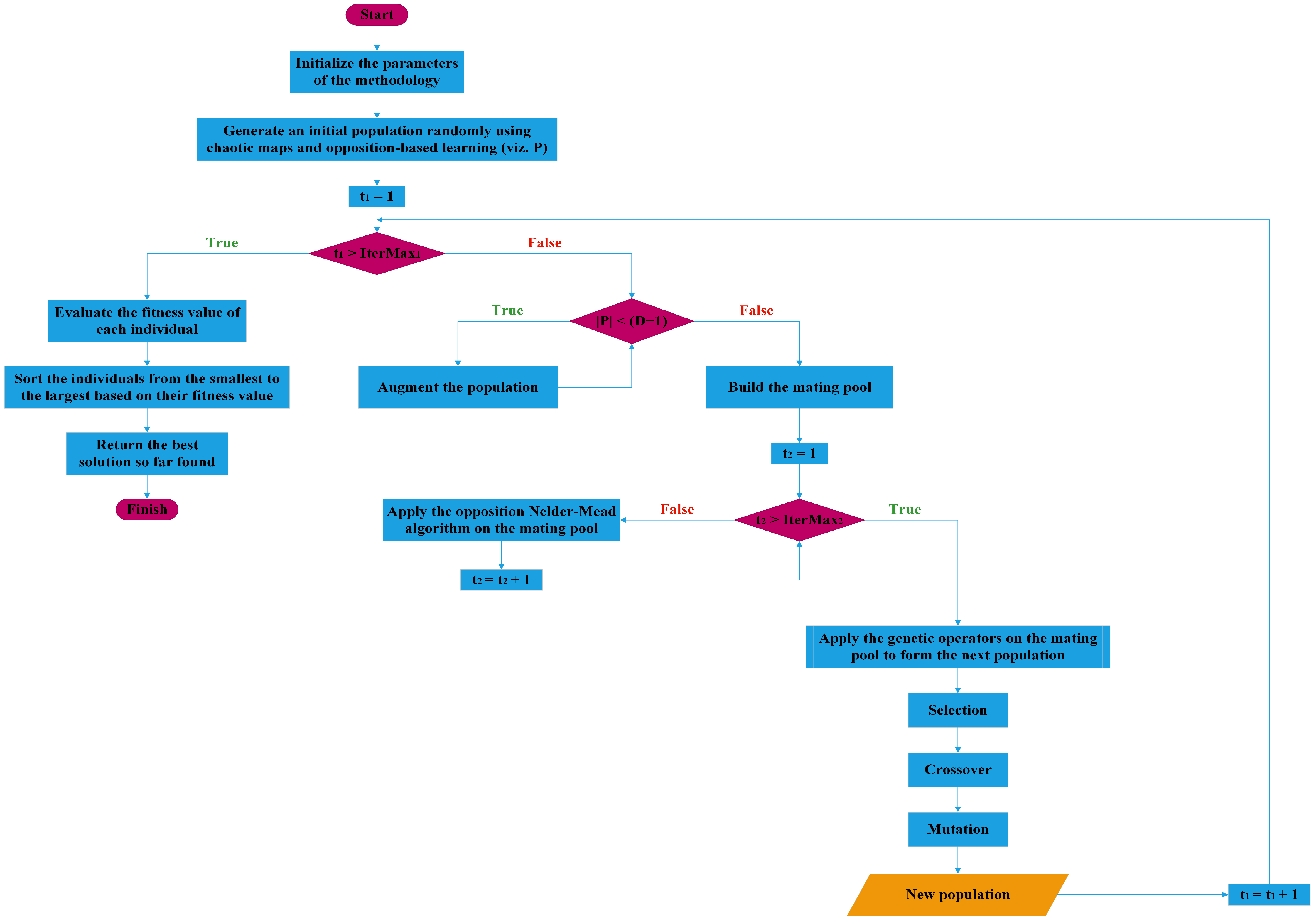
3. Proposed Methodology

In this section, we provide a comprehensive and detailed description of the proposed methodology, which involves the integration of the Nelder–Mead algorithm into the selection phase of the genetic algorithm. We delve into the specific steps and procedures involved in this integration, elucidating how the two algorithms interact and complement each other. Furthermore, we present the mathematical formulations and algorithms employed, providing a clear and systematic explanation of the modified selection process. By providing a thorough and meticulous description, we aim to ensure that readers have a comprehensive understanding of the proposed methodology and its underlying mechanisms. The flowchart presented in Figure 1 depicts the main phases of the proposed methodology. In the subsequent sections, we provide a detailed description of each phase.

3.1. Phase 1: Initialization of Parameters

The initial phase of our methodology involves the crucial step of parameter initialization, which lays the foundation for the subsequent stages. In this phase, we meticulously define and set the values of the parameters that govern the different algorithms and techniques of the proposed methodology. These parameters act as the guiding principles and variables that influence its behavior and performance. It is essential to establish appropriate initial values for these parameters, as they significantly impact the overall effectiveness and accuracy of the subsequent computations. Thus, by conscientiously determining the initial values, we ensure a solid starting point for our methodology, enabling reliable and meaningful results throughout the entire process. The parameters and symbols used are:

• D: The dimensionality of the search space.
• N: The population size.
• $x_{min}^{\left(j\right)}$: The component $x^{\left(j\right)}$ of vector $\mathbf{x}$ is bounded below by $x_{min}^{\left(j\right)}$.
• $x_{max}^{\left(j\right)}$: The component $x^{\left(j\right)}$ of vector $\mathbf{x}$ is bounded above by $x_{max}^{\left(j\right)}$.
• $\mathcal{N}(\mu ,\sigma )$: The normal distribution with mean $\mu$ and variance $\sigma$.
• $\mathrm{B}\mathrm{e}\mathrm{t}\mathrm{a}(\alpha ,\beta )$: The beta distribution, where $\alpha$ and $\beta$ are real numbers.
• $\mathrm{I}\mathrm{t}\mathrm{e}\mathrm{r}\mathrm{M}\mathrm{a}{\mathrm{x}}_1$: The maximum number of iterations for the GA.
• $\mathrm{I}\mathrm{t}\mathrm{e}\mathrm{r}\mathrm{M}\mathrm{a}{\mathrm{x}}_2$: The maximum number of iterations for the Nelder–Mead algorithm.
• $\rho$: The coefficients of reflection.
• $\chi$: The coefficients of expansion.
• $\gamma$: The coefficients of contraction.
• $\sigma$: The coefficients of shrinkage.
• $r_c$: The probability of performing crossover between pairs of selected individuals during reproduction.
• $r_m$: The probability of introducing random changes or mutations in the offspring to promote diversity.

3.2. Phase 2: Generation of the First Population

Chaotic maps are employed to initialize the first population in metaheuristics. These maps provide a stochastic and highly randomized approach to generating diverse and exploratory initial solutions within the search space. By leveraging the chaotic dynamics of these maps, initial population agents are assigned initial positions in a manner that ensures wide coverage and dispersion across the solution space. This initial diversity is essential for promoting exploration and preventing premature convergence, allowing the metaheuristic algorithm to effectively explore the search space and discover promising regions that may contain optimal or near-optimal solutions. By incorporating chaotic maps in the initialization process, our methodology can enhance its ability to escape local optima and improve the overall performance and convergence characteristics. Equation (10) serves as a fundamental tool for generating the positions of individuals within the initial population.

$${\mathbf{x}}_i=[{\phi }_i^{\left(1\right)}(x_{max}^{\left(1\right)}-x_{min}^{\left(1\right)})+x_{min}^{\left(1\right)},\dots ,{\phi }_i^{\left(D\right)}(x_{max}^{\left(D\right)}-x_{min}^{\left(D\right)})+x_{min}^{\left(D\right)}],i\in \{1,\dots ,N\}$$

(10)

We compare seven distinct chaotic schemes [67], which are Tent (Equation (11)), Sinusoidal (Equation (12)), Iterative (Equation (13)), Singer (Equation (14)), Sine (Equation (15)), Chebyshev (Equation (16)), and Circle maps (Equation (17)), to determine which one exhibits the best performance. The initial term ${\phi }_1$ of the chaotic sequence ${\phi }_1,\dots ,{\phi }_N$ is a random number drawn from the interval $[0,1]$.

$${\phi }_{z+1}=\left\{\begin{array}{ccc}\frac{{\phi }_z}{0.7}\hfill & ,\hfill & {\phi }_z<0.7\hfill \\ & \hfill & \\ \frac{10}{3}(1-{\phi }_z)\hfill & ,\hfill & {\phi }_z\ge 0.7\hfill \end{array}\right.$$

(11)

$${\phi }_{z+1}=2.3{\phi }_z^{2}sin\left(\pi {\phi }_z\right)$$

(12)

$${\phi }_{z+1}=sin\left(\frac{0.7\pi }{{\phi }_z}\right)$$

(13)

$${\phi }_{z+1}=\mu \left(7.86{\phi }_z-23.31{\phi }_z^2+28.75{\phi }_z^3-13.302875{\phi }_z^4\right),\mu =1.07$$

(14)

$${\phi }_{z+1}=sin\left(\pi {\phi }_z\right)$$

(15)

$${\phi }_{z+1}=cos\left(z{cos}^{-1}{\phi }_z\right)$$

(16)

$${\phi }_{z+1}=mod({\phi }_z+0.2-\left(\frac{0.5}{2\pi }\right)sin\left(2\pi {\phi }_z\right),1)$$

(17)

Although chaotic maps have proven to be useful in generating population members with higher diversity levels, they can lead to the initialization of candidate solutions that are far from the global optimum, particularly in real-world optimization problems where the global optimum is often unknown. This undesirable situation can impede the rapid convergence of solutions toward promising regions in the search space, compromising the algorithm’s convergence characteristics. To address these limitations of chaotic maps, an OBL strategy is incorporated into the initialization scheme of our methodology. The purpose of this strategy is to explore the broader coverage of the search space by searching for the opposite information of the chaotic population. The inclusion of OBL allows for the simultaneous evaluation of the original chaotic population and its opposite information, thereby increasing the probability of finding fitter solutions in the search space. We compare six distinct OBL strategies, named Strategy 1 [65] (Equation (18)), Strategy 2 [68] (Equation (19)), Strategy 3 [69] (Equation (20)), Strategy 4 [70] (Equation (21)), Strategy 5 [71] (Equation (22)), and Strategy 6 [71] (Equation (23)), to determine which one exhibits the best performance. Let $\mathbf{x}=[x^{\left(1\right)},\dots ,x^{\left(D\right)}]$ be a point in the n-dimensional space, where $x^{\left(1\right)},\dots ,x^{\left(D\right)}$ are real numbers and $x^{\left(j\right)}\in [x_{min}^{\left(j\right)},x_{max}^{\left(j\right)}],j=1,\dots ,D$. The opposite point of $\mathbf{x}$ is denoted by $\breve{\mathbf{x}}=[{\breve{x}}^{\left(1\right)},\dots ,{\breve{x}}^{\left(D\right)}]$ and can be calculated using one of Equations (18)–(22), or (23).

$${\breve{x}}^{\left(j\right)}=x_{min}^{\left(j\right)}+x_{max}^{\left(j\right)}-x^{\left(j\right)}$$

(18)

$${\breve{x}}^{\left(j\right)}=\mathrm{r}\mathrm{a}\mathrm{n}\mathrm{d}\left(\frac{x_{min}^{\left(j\right)}+x_{max}^{\left(j\right)}}{2},x_{min}^{\left(j\right)}+x_{max}^{\left(j\right)}-x^{\left(j\right)}\right)$$

(19)

$${\breve{x}}^{\left(j\right)}=\frac{x_{min}^{\left(j\right)}+x_{max}^{\left(j\right)}}{2}+\left({\upsilon }^{\left(j\right)}cos\left(\pi \mathcal{N}(1,0.25)\right)-{\nu }^{\left(j\right)}sin\left(\pi \mathcal{N}(1,0.25)\right)\right)$$

(20)

$${\upsilon }^{\left(j\right)}=x^{\left(j\right)}-\frac{x_{min}^{\left(j\right)}+x_{max}^{\left(j\right)}}{2}$$

$${\nu }^{\left(j\right)}=\sqrt{(x^{\left(j\right)}-x_{min}^{\left(j\right)})(x_{max}^{\left(j\right)}-x^{\left(j\right)})}$$

$${\breve{\mathbf{x}}}_i=2\times \left(\frac{{\mathbf{x}}_1+\dots +{\mathbf{x}}_N}{N}\right)-{\mathbf{x}}_i$$

(21)

$${\breve{x}}^{\left(j\right)}=(x_{max}^{\left(j\right)}-x_{min}^{\left(j\right)})·\mathrm{B}\mathrm{e}\mathrm{t}\mathrm{a}(\alpha ,\beta )+x_{min}^{\left(j\right)}$$

(22)

$${\breve{x}}^{\left(j\right)}=(x_{max}^{\left(j\right)}-x_{min}^{\left(j\right)})·\mathrm{B}\mathrm{e}\mathrm{t}\mathrm{a}(\alpha ,\beta )+x_{min}^{\left(j\right)}$$

(23)

$$\alpha =\left\{\begin{array}{ccc}s·p\hfill & ,\hfill & M<0.5\hfill \\ s\hfill & ,\hfill & M\ge 0.5\hfill \end{array}\right.$$

$$\beta =\left\{\begin{array}{ccc}s\hfill & ,\hfill & M<0.5\hfill \\ s·p\hfill & ,\hfill & M\ge 0.5\hfill \end{array}\right.$$

$$s={\left(\frac{1}{\sqrt{\nu }}\right)}^{1+\mathcal{N}(0,0.5)},\mathrm{f}\mathrm{o}\mathrm{r} \mathrm{E}\mathrm{q}\mathrm{u}\mathrm{a}\mathrm{t}\mathrm{i}\mathrm{o}\mathrm{n}\left(22\right)$$

$$s=0.1\sqrt{\nu }+0.9,\mathrm{f}\mathrm{o}\mathrm{r} \mathrm{E}\mathrm{q}\mathrm{u}\mathrm{a}\mathrm{t}\mathrm{i}\mathrm{o}\mathrm{n}\left(23\right)$$

$$p=\left\{\begin{array}{ccc}\frac{(s-2)M+1}{s(1-M)}\hfill & ,\hfill & M<0.5\hfill \\ \hfill & \hfill & \\ \frac{2-s}{s}+\frac{s-1}{s·M}\hfill & ,\hfill & M\ge 0.5\hfill \end{array}\right.$$

$$M=\frac{x_{max}^{\left(j\right)}-x^{\left(j\right)}}{x_{max}^{\left(j\right)}-x_{min}^{\left(j\right)}},\mathrm{f}\mathrm{o}\mathrm{r} \mathrm{E}\mathrm{q}\mathrm{u}\mathrm{a}\mathrm{t}\mathrm{i}\mathrm{o}\mathrm{n}\left(22\right)$$

$$M=\frac{x^{\left(j\right)}-x_{min}^{\left(j\right)}}{x_{max}^{\left(j\right)}-x_{min}^{\left(j\right)}},\mathrm{f}\mathrm{o}\mathrm{r} \mathrm{E}\mathrm{q}\mathrm{u}\mathrm{a}\mathrm{t}\mathrm{i}\mathrm{o}\mathrm{n}\left(23\right)$$

$$\nu =\frac{1}{N}\sum _{i=1}^N\underset{\mathbf{c}\in \{{\mathbf{x}}_1,\dots ,{\mathbf{x}}_N\}-\left\{{\mathbf{x}}_i\right\}}{argmin}\sqrt{\frac{1}{D}\sum _{j=1}^D{\left(\frac{x^{\left(j\right)}-c^{\left(j\right)}}{x_{max}^{\left(j\right)}-x_{min}^{\left(j\right)}}\right)}^2}$$

Algorithm 1 serves as a valuable tool for demonstrating the operational principles of the initialization phase within our methodology. By presenting a step-by-step procedure, it effectively showcases how the initial population of candidate solutions is generated. Through Algorithm 1, we highlight the specific techniques and strategies employed to create a diverse and representative set of individuals at the beginning of the optimization process. It is worth pointing out that if a candidate solution exceeds the boundaries of the search space after undergoing an opposition operation, it is subsequently restored to within the valid range utilizing Equation (24).

$$\left\{\begin{array}{ccc}{x}^{\left(j\right)}\leftarrow x_{max}^{\left(j\right)}\hfill & ,\hfill & x^{\left(j\right)}>x_{max}^{\left(j\right)}\hfill \\ x^{\left(j\right)}\leftarrow x_{min}^{\left(j\right)}\hfill & ,\hfill & x^{\left(j\right)}<x_{min}^{\left(j\right)}\hfill \end{array}\right.$$

(24)

Algorithm 1: The pseudocode for the initialization phase of our methodology.
	Input: D: The dimensionality of the search space.
	Input: N: The population size.
	Input: $x_{min}^{\left(1\right)},\dots ,x_{min}^{\left(D\right)}$: The lower boundaries of entries $x^{\left(1\right)},\dots ,x^{\left(D\right)}$.
	Input: $x_{max}^{\left(1\right)},\dots ,x_{max}^{\left(D\right)}$: The upper boundaries of entries $x^{\left(1\right)},\dots ,x^{\left(D\right)}$.
	Input: $f(.)$: The multivariate function to be minimized.
1	for $i\leftarrow 1$ to N do
2		for $j\leftarrow 1$ to D do
3			if ($i=1$) then
4				${\phi }_i^{\left(j\right)}\leftarrow \mathrm{rand}(0,1)$
5			end
6			else
7				${\phi }_i^{\left(j\right)}$ is updated using the selected chaotic map (Equations (11)–(16) or (17);
8			end
9		end
10		Compute ${\mathbf{x}}_i$ using Equation (10);
11		Compute ${\breve{\mathbf{x}}}_i$ using the selected opposition-based learning strategy (Equations (18)–(22) or (23);
12		${\mathbf{x}}_i\leftarrow argmin\{f\left({\mathbf{x}}_i\right),f\left({\breve{\mathbf{x}}}_i\right)\}$;
13	end

3.3. Phase 3: Augmentation of the Population

The Nelder–Mead algorithm requires the construction of a simplex with exactly $D+1$ vertices, where D represents the dimensionality of the problem. However, in some cases, the number of individuals available in the initial population is smaller than $D+1$, i.e., $N<(D+1)$. To overcome this limitation and enable the application of the Nelder–Mead algorithm, we augment the population size by generating additional individuals. By introducing these extra individuals, we ensure that the simplex can be properly formed, allowing the algorithm to proceed as intended. This augmentation step ensures that the optimization process can fully leverage the capabilities of the Nelder–Mead algorithm, even when the initial population size is insufficient to construct the required simplex.

In optimization, when the population size is insufficient or does not meet the requirements of certain algorithms, techniques can be employed to augment or expand the population. These techniques aim to increase the diversity, coverage, or exploration capabilities of the population to enhance the optimization process. Some common techniques used to augment a population in optimization include:

• Scaling: Scaling a vector $\mathbf{x}$ in an n-dimensional search space involves adjusting the magnitude of its components uniformly. Mathematically, the scaled vector $\acute{\mathbf{x}}$ can be obtained by multiplying each component of the original vector $\mathbf{x}$ by a scaling factor s (Equation (25)) [72].

  $$\acute{\mathbf{x}}=s\times \mathbf{x}$$

  (25)

  where $\mathbf{x}$ represents the original vector in n-dimensional space, and $\acute{\mathbf{x}}$ represents the scaled vector. The scaling factor s determines the magnitude of the scaling applied to the vector, allowing for the contraction ($s<1$) or expansion ($s>1$) of its length. In our methodology, the scaling factor s is generated randomly from the normal distribution $\mathcal{N}(0,1-\frac{t_1}{{\mathrm{IterMax}}_1})$.
• Rotation: Rotating a vector $\mathbf{x}$ in an n-dimensional search space involves changing its direction or orientation while preserving its magnitude. Mathematically, the rotated vector $\acute{\mathbf{x}}$ can be obtained by multiplying the original vector $\mathbf{x}$ by a rotation matrix R (Equation (26)) [72].

  $$\acute{\mathbf{x}}=R\times \mathbf{x}$$

  (26)

  $$R=\left\{\begin{array}{ccc}{r}_{kk}=1\hfill & ,\hfill & k\notin \{p,q\}\hfill \\ r_{kk}=cos\theta \hfill & ,\hfill & k\in \{p,q\}\hfill \\ r_{ij}=0\hfill & ,\hfill & \mathrm{otherwise}\hfill \\ r_{xy}=sin\theta \hfill & \hfill & \\ r_{yx}=-sin\theta \hfill & \hfill & \end{array}\right.$$

  where $\mathbf{x}$ represents the original vector in the n-dimensional space, $\acute{\mathbf{x}}$ represents the rotated vector, p and q represent the spanned plane, and $\theta$ is the rotation angle. The rotation matrix R depends on the specific rotation operation being applied and is typically constructed using a combination of trigonometric functions, such as sine and cosine, to represent the desired rotation angles and axes in the n-dimensional space. In our methodology, the rotation angle $\theta$ is computed using the expression $\theta =\mathcal{B}\left(0.5\right)·\mathrm{r}\mathrm{a}\mathrm{n}\mathrm{d}(-\pi ,\pi )$, where the term $\mathcal{B}\left(0.5\right)$ denotes the Bernoulli distribution with a probability of success equal to 0.5.
• Translation: Translating a vector $\mathbf{x}$ in an n-dimensional search space involves shifting its position without changing its direction or magnitude. Mathematically, the translated vector $\acute{\mathbf{x}}$ can be obtained by adding a translation vector $\mathbf{t}$ to the original vector $\mathbf{x}$ (Equation (27)) [72].

  $$\acute{\mathbf{x}}=\mathbf{x}+\mathbf{t}$$

  (27)

  where $\mathbf{x}$ represents the original vector in the n-dimensional space, $\acute{\mathbf{x}}$ represents the translated vector, and $\mathbf{t}$ represents the translation vector. The translation vector $\mathbf{t}$ contains the amounts by which each component of the original vector is shifted along its respective axes. In our methodology, the vector $\mathbf{t}$ is generated randomly from the normal distribution $\mathcal{N}(0,1-\frac{t_1}{\mathrm{I}\mathrm{t}\mathrm{e}\mathrm{r}\mathrm{M}\mathrm{a}{\mathrm{x}}_1})$.
• Reflection: Reflecting a vector $\mathbf{x}$ in an n-dimensional search space involves creating its mirror image across a specified line or plane while preserving its magnitude. Mathematically, the reflected vector $\acute{\mathbf{x}}$ can be obtained by subtracting the original vector $\mathbf{x}$ from the double of the projection of $\mathbf{x}$ onto the reflection line or plane (Equation (28)) [72].

  $$\acute{\mathbf{x}}=2\times (\mathbf{x}·\mathbf{v})\times \mathbf{v}-\mathbf{x}$$

  (28)

  where $\mathbf{x}$ represents the original vector in the n-dimensional space, $\acute{\mathbf{x}}$ represents the reflected vector, $\mathbf{v}$ represents the normal vector of the reflection line or plane, and · denotes the dot product between two vectors. The reflection operation effectively flips the sign of the component along the reflection axis, resulting in the mirror image of the original vector. In our methodology, the vector $\mathbf{v}$ is generated randomly from the normal distribution $\mathcal{N}(0,1-\frac{t_1}{\mathrm{I}\mathrm{t}\mathrm{e}\mathrm{r}\mathrm{M}\mathrm{a}{\mathrm{x}}_1})$.
• Similarity transformation: The similarity transformation of a vector $\mathbf{x}$ in an n-dimensional search space involves scaling and rotating the vector while preserving its shape. Mathematically, the transformed vector $\acute{\mathbf{x}}$ can be obtained by first scaling the original vector $\mathbf{x}$ by a scaling factor s and then rotating it using a rotation matrix R (Equation (29)) [72].

  $$\acute{\mathbf{x}}=s\times R\times \mathbf{x}$$

  (29)

  where $\mathbf{x}$ represents the original vector in the n-dimensional space, $\acute{\mathbf{x}}$ represents the transformed vector, s is the scaling factor, and R is the rotation matrix. The similarity transformation allows for modifications in size and orientation while preserving the relative positions of the vector’s components.

Algorithm 2 serves as a concise representation, capturing the key stages of the augmentation phase. This algorithm effectively distills the fundamental procedures and essential processes involved in augmenting a given population. By encapsulating the primary steps in a succinct form, Algorithm 2 enables a clear understanding of the augmentation phase, offering a compact yet comprehensive guide for implementing this crucial component of our methodology. It is worth mentioning that if the generated candidate solution exceeds the boundaries of the search space after undergoing a geometric transformation, it is subsequently restored to within the valid range utilizing Equation (24).

Algorithm 2: The pseudocode for the augmentation phase of our methodology.
	Input: D: The dimensionality of the search space.
	Input: $x_{min}^{\left(1\right)},\dots ,x_{min}^{\left(D\right)}$: The lower boundaries of entries $x^{\left(1\right)},\dots ,x^{\left(D\right)}$.
	Input: $x_{max}^{\left(1\right)},\dots ,x_{max}^{\left(D\right)}$: The upper boundaries of entries $x^{\left(1\right)},\dots ,x^{\left(D\right)}$.
	Input: $P=\{{\mathbf{x}}_1,\dots ,{\mathbf{x}}_N\}$: The candidate solutions within the current population.
1	while $\left(\left|P\right|<(D+1)\right)$ do
2		Select a random vector ${\mathbf{x}}_r$, where $r\in \{1,\dots ,|P\left|\right\}$, using roulette-wheel selection;
3		Compute the vector ${\acute{\mathbf{x}}}_r$ using the selected augmentation operation (Equations (25)–(28) or (29);
4		Compute ${\breve{\stackrel{´}{\mathbf{x}}}}_r$ using the selected opposition-based learning strategy (Equations (18)–(22) or (23);
5		${\acute{\mathbf{x}}}_r\leftarrow argmin\{f\left({\acute{\mathbf{x}}}_r\right),f\left({\breve{\stackrel{´}{\mathbf{x}}}}_r\right)\}$;
6		Add the new vector ${\acute{\mathbf{x}}}_r$ to the population P;
7	end

3.4. Phase 4: Building the Mating Pool

During this phase, the individuals within the population undergo a sorting process to identify the most promising candidates. The goal is to select $D+1$ candidate solutions, where D represents the dimensionality of the problem. These selected individuals will serve as the entry points for the subsequent application of the opposition Nelder–Mead algorithm. By carefully sorting and choosing these initial candidates, the mating pool is effectively formed, paving the way for further optimization and refinement through the proposed methodology. This critical phase ensures that the subsequent steps of our methodology are initiated with a set of highly competitive solutions, maximizing the potential for successful optimization and convergence.

In the process of building the mating pool, we employ the roulette-wheel selection method [73]. The specific approach varies depending on the size of the population. In the case where the population size is equal to or less than $D+1$, we apply roulette-wheel selection to the augmented population. This augmented population includes additional individuals that have been generated to meet the minimum population size requirement. However, if the population size exceeds $D+1$, we solely utilize roulette-wheel selection on the current population without any augmentation.

3.5. Phase 5: Application of the Opposition Nelder–Mead Algorithm

Algorithm 3 serves as a demonstration of the working principle underlying the opposition Nelder–Mead algorithm, which plays a pivotal role in our methodology. By following the steps outlined in Algorithm 3, we can witness firsthand how the opposition Nelder–Mead algorithm operates to optimize a given objective function. This algorithm showcases the dynamic interplay between reflection, expansion, contraction, and shrinking, allowing us to iteratively refine and improve the selection phase of the GA. Algorithm 3 encapsulates the essence of the opposition Nelder–Mead algorithm’s working principle, providing a clear and practical illustration of its effectiveness in guiding the selection phase of the GA on the one hand, and the optimization process within our methodology on the other hand. It is worth mentioning that if a vertex exceeds the boundaries of the search space after undergoing the operations described in Algorithm 3, it is consequently restored to within the valid range using Equation (24).

$${\mathbf{y}}_1=\underset{{\mathbf{x}}_i\in \{{\mathbf{x}}_1,\dots ,{\mathbf{x}}_{D+1}\}}{argmin}\left\{f\left({\mathbf{x}}_i\right)\right\}$$

(30)

$${\mathbf{y}}_{D+1}=\underset{{\mathbf{x}}_i\in \{{\mathbf{x}}_1,\dots ,{\mathbf{x}}_{D+1}\}}{argmax}\left\{f\left({\mathbf{x}}_i\right)\right\}$$

(31)

$${\mathbf{y}}_D=\underset{{\mathbf{x}}_i\in \{{\mathbf{x}}_1,\dots ,{\mathbf{x}}_{D+1}\}-\left\{{\mathbf{y}}_{D+1}\right\}}{argmax}\left\{f\left({\mathbf{x}}_i\right)\right\}$$

(32)

$$\overline{\mathbf{x}}=\frac{1}{D}\sum _{{\mathbf{x}}_i\in \{{\mathbf{x}}_1,\dots ,{\mathbf{x}}_{D+1}\}-\left\{{\mathbf{y}}_{D+1}\right\}}{\mathbf{x}}_i$$

(33)

Algorithm 3: The pseudocode for the opposition Nelder–Mead algorithm.
	Input: $x_{min}^{\left(1\right)},\dots ,x_{min}^{\left(D\right)}$: The lower boundaries of entries $x^{\left(1\right)},\dots ,x^{\left(D\right)}$.
	Input: $x_{max}^{\left(1\right)},\dots ,x_{max}^{\left(D\right)}$: The upper boundaries of entries $x^{\left(1\right)},\dots ,x^{\left(D\right)}$.
	Input: $\{{\mathbf{x}}_1,\dots ,{\mathbf{x}}_{D+1}\}$: The candidate solutions within the mating pool.
	Input: $\rho$, $\chi$, $\gamma$, and $\sigma$: The coefficients of reflection, expansion, contraction, and shrinkage, respectively.
	Input: $f(.)$: The multivariate function to be minimized.
1	for $t_2\leftarrow 1$ to $IterMa{x}_2$ do
2		Compute the best vertex ${\mathbf{y}}_1$ using Equation (30);
3		Compute the worst vertex ${\mathbf{y}}_{D+1}$ using Equation (31);
4		Compute the next-worst vertex ${\mathbf{y}}_D$ using Equation (32);
5		Compute the centroid $\overline{\mathbf{x}}$ excluding the worst vertex using Equation (33);
6		Compute the reflection vertex ${\mathbf{x}}_r$ using Equation (5);
7		Compute ${\breve{\mathbf{x}}}_r$ using the selected opposition-based learning strategy (Equations (18)–(22) or (23);
8		if $\left(f\left({\mathbf{y}}_1\right)\le f\left({\mathbf{x}}_r\right)<f\left({\mathbf{y}}_D\right)\right)$ then
9			${\mathbf{x}}_{D+1}\leftarrow argmin\{f\left({\mathbf{x}}_r\right),f\left({\breve{\mathbf{x}}}_r\right)\}$;
10		end
11		if $\left(f\left({\mathbf{x}}_r\right)<f\left({\mathbf{y}}_1\right)\right)$ then
12			Compute the expansion vertex ${\mathbf{x}}_e$ using Equation (6);
13			Compute ${\breve{\mathbf{x}}}_e$ using the selected opposition-based learning strategy (Equations (18)–(22) or (23);
14			if $\left(f\left({\mathbf{x}}_e\right)<f\left({\mathbf{x}}_r\right)\right)$ then
15				${\mathbf{x}}_{D+1}\leftarrow argmin\{f\left({\mathbf{x}}_e\right),f\left({\breve{\mathbf{x}}}_e\right)\}$
16			end
17			else
18				${\mathbf{x}}_{D+1}\leftarrow argmin\{f\left({\mathbf{x}}_r\right),f\left({\breve{\mathbf{x}}}_r\right)\}$
19			end
20		end
21		if $\left(f\left({\mathbf{x}}_r\right)\ge f\left({\mathbf{y}}_D\right)\right)$ then
22			if $\left(f\left({\mathbf{y}}_D\right)\le f\left({\mathbf{x}}_r\right)<f\left({\mathbf{y}}_{D+1}\right)\right)$ then
23				Compute the outside contraction vertex ${\mathbf{x}}_{oc}$ using Equation (7);
24				Compute ${\breve{\mathbf{x}}}_{oc}$ using the selected opposition-based learning strategy (Equations (18)–(22) or (23);
25				if $\left(f\left({\mathbf{x}}_{oc}\right)<f\left({\mathbf{x}}_r\right))\right)$ then
26					${\mathbf{x}}_{D+1}\leftarrow argmin\{f\left({\mathbf{x}}_{oc}\right),f\left({\breve{\mathbf{x}}}_{oc}\right)\}$
27				end
28			end
29			if $\left(f\left({\mathbf{x}}_r\right)\ge f\left({\mathbf{y}}_{D+1}\right)\right)$ then
30				Compute the inside contraction vertex ${\mathbf{x}}_{ic}$ using Equation (8);
31				Compute ${\breve{\mathbf{x}}}_{ic}$ using the selected opposition-based learning strategy (Equations (18)–(22) or (23);
32				if $\left(f\left({\mathbf{x}}_{ic}\right)<f\left({\mathbf{y}}_{D+1}\right)\right)$ then
33					${\mathbf{x}}_{D+1}\leftarrow argmin\{f\left({\mathbf{x}}_{ic}\right),f\left({\breve{\mathbf{x}}}_{ic}\right)\}$
34				end
35			end
36		end
37		for ${\mathbf{x}}_i\in \{{\mathbf{x}}_1,\dots ,{\mathbf{x}}_{D+1}\}$ do
38			Update the vertex ${\mathbf{x}}_i$ using Equation (9);
39			Compute ${\breve{\mathbf{x}}}_i$ using the selected opposition-based learning strategy (Equations (18)–(22) or (23);
40			${\mathbf{x}}_i\leftarrow argmin\{f\left({\mathbf{x}}_i\right),f\left({\breve{\mathbf{x}}}_i\right)\}$
41		end
42	end

3.6. Phase 6: Application of Genetic Operators

The presented study provides a comprehensive understanding of the GA by delineating its key components into distinct sections. Section 3.6.1 elucidates the intricate details of the selection process, where individuals from the population are carefully chosen to pass on to the next generation. Section 3.6.2 focuses on the reproduction process, outlining how the selected parents generate offspring through recombination operations. Lastly, in Section 3.6.3, the mutation process takes center stage, elucidating the mechanisms through which the genetic material of the individuals undergoes random modifications to introduce novel genetic information. It is worth pointing out that if an individual exceeds the boundaries of the search space after undergoing the genetic operators, it is consequently restored to within the valid range using Equation (24).

3.6.1. Selection

Genetic algorithms are a type of evolutionary algorithm that mimics the process of natural selection to solve optimization problems. In GAs, the selection mechanism determines which individuals from a given population will be passed to the next generation. The selection process is crucial in driving the search for better solutions over successive generations. Several common selection mechanisms are used in GAs [74]. In our methodology, we use elitism [75]. Elitism involves selecting a certain number of the best individuals from the current population and directly transferring them to the next generation without any changes. This ensures that the best solutions found so far are preserved across generations, preventing the loss of fitness during the evolution process.

3.6.2. Crossover

The crossover technique used to deal with continuous values in genetic algorithms is known as BLX-$\alpha$ (Blend Crossover) [76]. BLX-$\alpha$ is a variation of the traditional crossover operator used in genetic algorithms, which is typically designed for binary or discrete variables. BLX-$\alpha$ allows for the combination of parent solutions that have continuous values.

In the BLX-$\alpha$ crossover, a new offspring is created by blending the values of corresponding variables from two parent solutions. The process involves selecting a random value within a defined range for each variable and using the blending factor to determine the range of values for the offspring. The blending factor, denoted as alpha ($\alpha$), controls the amount of exploration and exploitation during the crossover process. The following steps present a high-level description of the BLX-$\alpha$ crossover technique used in our methodology. Steps 1, 2, and 3 are iteratively performed until the size of the next population becomes N. It is worth highlighting that two parent individuals will undergo a crossover process based on a specified crossover rate ($r_c$):

• Select two parent individuals ${\mathbf{x}}_{p_1}$ and ${\mathbf{x}}_{p_2}$ from the mating pool using roulette-wheel selection [73].
• Compute the offspring ${\mathbf{x}}_o$ using Equation (34).

  $${\mathbf{x}}_o=[\mathrm{r}\mathrm{a}\mathrm{n}\mathrm{d}({\lambda }_1-\alpha {\pi }_i,{\omega }_1+\alpha {\pi }_i),\dots ,\mathrm{r}\mathrm{a}\mathrm{n}\mathrm{d}({\lambda }_D-\alpha {\pi }_D,{\omega }_D+\alpha {\pi }_D)]$$

  (34)

  $${\lambda }_j=min(x_{p_1}^{\left(j\right)},x_{p_2}^{\left(j\right)})$$

  $${\omega }_j=max(x_{p_1}^{\left(j\right)},x_{p_2}^{\left(j\right)})$$

  $${\pi }_j=|{\omega }_j-{\lambda }_j|$$

  $$\alpha =1-\mathrm{r}\mathrm{a}\mathrm{n}\mathrm{d}(0,1)\times \left(1-\frac{t_1}{\mathrm{I}\mathrm{t}\mathrm{e}\mathrm{r}\mathrm{M}\mathrm{a}{\mathrm{x}}_1}\right)$$
• Add the new offspring to the next population.

The value of $\alpha$ determines the extent of exploration and exploitation during crossover. A smaller value of $\alpha$ encourages more exploration, allowing for a wider range of values in the offspring. Conversely, a larger value of $\alpha$ encourages more exploitation, resulting in offspring closer to the parent solutions. The BLX-$\alpha$ crossover technique enables the combination of continuous variables in genetic algorithms and provides a way to effectively explore and exploit the search space.

3.6.3. Mutation

The mutation technique, commonly used to deal with continuous values in genetic algorithms, is known as Gaussian mutation or normal distribution mutation [77]. This technique introduces random perturbations to the values of the variables in a continuous search space, mimicking the behavior of a Gaussian or normal distribution. In Gaussian mutation, a random value is generated from a Gaussian distribution with a mean of zero and a predefined standard deviation. This random value is then added to each variable of an individual in the population, causing a small random change in its value. The standard deviation determines the magnitude of the mutation, controlling the exploration and exploitation trade-off during the search process. It is worth emphasizing that an individual will undergo a mutation process based on a designated mutation rate ($r_m$). The following steps introduce a high-level description of the Gaussian mutation technique used in our methodology:

• For each variable in an individual, generate a random value from a Gaussian distribution with a mean of zero and a predefined standard deviation.

  $$\sigma =\left(1-\frac{t_1}{\mathrm{I}\mathrm{t}\mathrm{e}\mathrm{r}\mathrm{M}\mathrm{a}{\mathrm{x}}_1}\right)$$
• Generate a random number drawn from the uniform distribution. If the generated number is less than or equal to the specified mutation rate, then add the mutation amount to the current value of the variable to obtain the mutated value.
• Repeat steps 1 and 2 for all individuals in the population.

The standard deviation parameter plays a crucial role in Gaussian mutation. A smaller standard deviation leads to smaller random perturbations, resulting in finer exploration and a higher likelihood of converging to a local optimum. Conversely, a larger standard deviation allows for larger random perturbations, promoting broader exploration and the potential to escape local optima. Gaussian mutation enables the exploration of the continuous search space in genetic algorithms by introducing random perturbations to the individuals. It provides a way to balance exploration and exploitation, aiding the algorithm’s ability to search for optimal or near-optimal solutions in continuous domains.

3.7. Time Complexity of the Proposed Methodology

In this section, we delve into the time complexity of the proposed methodology. The efficiency of the methodology is intricately tied to its various phases, namely Phase 2, Phase 3, Phase 4, Phase 5, and Phase 6. The time complexity analysis of each stage provides valuable insights into the overall performance of the methodology. By understanding the time complexities of these individual stages, we gain a comprehensive understanding of how the methodology scales with larger dimensions or more complex problems. Through this examination, we can assess the computational demands and make informed decisions regarding the feasibility and efficiency of implementing the proposed methodology in real-world scenarios.

Table 1. Time complexity of the proposed methodology.

Phase	Time Complexity
Phase 2	$\mathcal{O}\left(n^3\right)$
Phase 3	$\mathcal{O}\left(n^3\right)$
Phase 4	$\mathcal{O}\left(n^3\right)$
Phase 5	$\mathcal{O}\left(n^3\right)$
Phase 6	$\mathcal{O}\left(n^3\right)$
Methodology’s time complexity	$\mathcal{O}\left(n^3\right)$

provides a comprehensive summary of the time complexity associated with each phase of the proposed methodology. Finally, by computing the complexities of all phases, we can determine the global complexity of the methodology. It is worth mentioning that the time complexity of a function evaluation is $\mathcal{O}\left(n^2\right)$.

4. Experimental Results and Discussion

The workstation utilized for conducting the experimental study is equipped with a well-suited hardware and software configuration to support the required tasks. The workstation runs on a Windows 11 Home operating system, providing a user-friendly interface and compatibility with a wide range of software applications. The hardware configuration features an Intel(R) Core(TM) i7-9750H CPU, with a base frequency of 2.60 GHz and a maximum turbo frequency of 4.50 GHz. This high-performance processor ensures the efficient execution of computational tasks and data processing. Additionally, the workstation includes 16.0 GB of RAM, enabling the handling of complex calculations with ease. The software suite installed on the workstation consists of Matlab R2020b, a powerful programming language and environment for numerical computing and algorithm development. Furthermore, the IBM SPSS Statistics 26 software is also installed on the workstation, providing a comprehensive platform for statistical analysis and conducting various statistical tests. This combination of hardware and software configurations offers a robust and capable environment for conducting the experimental study, effectively facilitating data analysis, statistical modeling, and computational tasks.

The effectiveness of the proposed methodology was assessed through rigorous testing on the CEC 2022 (https://github.com/P-N-Suganthan/2022-SO-BO (accessed on 28 June 2023)) benchmark, which comprises a set of 12 hard and challenging test functions. Among these functions, one is unimodal in nature, whereas four are multimodal. Additionally, three functions are designed as hybrid, and the remaining four functions are composite. The use of the unimodal function aims to evaluate the methodology’s exploitation capability, as it requires focusing on refining solutions within a simple search space. The inclusion of multimodal functions allows for assessing the methodology’s exploration capability, as it necessitates exploring a complex search space with multiple optima. Furthermore, the hybrid and composite functions were employed to evaluate the methodology’s ability to strike a balance between exploration and exploitation, as they combine different characteristics and complexities. The comprehensive testing on this diverse set of test functions provided valuable insights into the performance and robustness of the proposed methodology across various optimization scenarios.

Table 2. Information and features of the test problems suite.

	N°	Functions	${\mathit{F}}_{\mathit{i}}^{*}$
Unimodal function	1	Shifted and full Rotated Zakharov Function	300
Basic functions	2	Shifted and full Rotated Rosenbrock’s Function	400
	3	Shifted and full Rotated Expanded Schaffer’s $f_6$ Function	600
	4	Shifted and full Rotated Non-Continuous Rastrigin’s Function	800
	5	Shifted and full Rotated Lévy Function	900
Hybrid functions	6	Hybrid Function 1 (N = 3)	1800
	7	Hybrid Function 2 (N = 6)	2000
	8	Hybrid Function 3 (N = 5)	2200
Composition functions	9	Composition Function 1 (N = 5)	2300
	10	Composition Function 2 (N = 4)	2400
	11	Composition Function 3 (N = 5)	2600
	12	Composition Function 4 (N = 6)	2700
Search range: ${[-100,100]}^D$

D: The dimensionality of the search space.

depicts the features of the test problems suite.

To thoroughly assess the effectiveness of the proposed methodology, it was subjected to a comparative analysis against 11 highly influential and powerful algorithms, specifically:

• Co-PPSO: Performance of Composite PPSO on Single Objective Bound Constrained Numerical Optimization Problems of CEC 2022 [78].
• EA4eigN100-10: Eigen Crossover in Cooperative Model of Evolutionary Algorithms applied to CEC 2022 Single Objective Numerical Optimization [79].
• IMPML-SHADE: Improvement of Multi-Population ML-SHADE [80].
• IUMOEAII: An improved IMODE algorithm based on Reinforcement Learning [81].
• jSObinexpEig: An adaptive variant of jSO with multiple crossover strategies employing Eigen transformation [82].
• MTT-SHADE: Multiple Topology SHADE with a tolerance-based composite framework for CEC 2022 Single Objective Bound Constrained Numerical Optimization [83].
• NL-SHADE-LBC: NL-SHADE-LBC algorithm with linear parameter adaptation bias change for CEC 2022 Numerical Optimization [84].
• NL-SHADE-RSP-MID: A version of the NL-SHADE-RSP algorithm with Midpoint for CEC 2022 Single Objective Bound Constrained Problems [85].
• OMCSOMA: Opposite Learning and Multi-Migrating Strategy-Based Self-Organizing Migrating algorithm with a convergence monitoring mechanism [86].
• S-LSHADE-DP: Dynamic Perturbation for Population Diversity Management in Differential Evolution [87].
• NLSOMACLP: NL-SOMA-CLP for Real Parameter Single Objective Bound Constrained Optimization [88].

Each of these algorithms represents a significant approach in the field of optimization. The comparison was conducted by measuring and reporting the average and standard deviation values for each algorithm. This comprehensive evaluation allowed for a comprehensive understanding of the proposed methodology’s performance in relation to other well-established algorithms. By considering a diverse range of state-of-the-art algorithms, we were able to gain valuable insights into the strengths, weaknesses, and comparative performance of the proposed methodology. To enhance clarity, the algorithms originally labeled Co-PPSO are renamed $A_2$, and the algorithms originally labeled EA4eigN100-10 are renamed $A_3$. This renaming convention was also used for the remaining algorithms. By utilizing the new nomenclature ($A_2,A_3,\dots ,A_{12}$), the presentation and interpretation of the results are more straightforward and unambiguous. Finally, our methodology is renamed $A_1$.

Table 3. Different diversity measurements obtained for the chosen configurations.

	OBL Strategies	Equation (18)		Equation (19)		Equation (20)		Equation (21)		Equation (22)		Equation (23)
Chaotic Schemes		$\mathit{D}=\mathbf{10}$	$\mathit{D}=\mathbf{20}$	$\mathit{D}=\mathbf{10}$	$\mathit{D}=\mathbf{20}$	$\mathit{D}=\mathbf{10}$	$\mathit{D}=\mathbf{20}$	$\mathit{D}=\mathbf{10}$	$\mathit{D}=\mathbf{20}$	$\mathit{D}=\mathbf{10}$	$\mathit{D}=\mathbf{20}$	$\mathit{D}=\mathbf{10}$	$\mathit{D}=\mathbf{20}$
Equation (11)		38.67	39.45	33.89	32.74	44.32	45.24	37.59	36.75	43.48	43.38	45	46.17
Equation (12)		39.49	40.32	34.01	32.44	44.65	46.3	36.28	37.35	43.49	43.36	44.92	46.22
Equation (13)		38.22	39.43	34.28	32.56	44.44	45.95	37.33	37.31	43.48	43.37	45.15	45.61
Equation (14)		38.77	40.43	33.76	33.04	44.3	45.43	38.72	38.39	43.5	43.38	45.57	46.26
Equation (15)		38.77	39.88	33.91	32.56	44.2	45.54	37.9	38.19	43.5	43.37	45.4	45.95
Equation (16)		39.93	39.56	34.07	32.61	44.63	45.71	37.46	36.5	43.58	43.37	45.3	46.28
Equation (17)		39.73	40.15	33.66	33.11	44.79	45.32	37.25	38.02	43.49	43.37	45.14	46.05

presents the diversity measurements ($\Delta$) calculated using Equation (35) during the initialization of the initial population. The diversity values were examined for two different dimensions, $D=10$ and $D=20$. For $D=10$, it was observed that the highest diversity value was achieved when employing the chaotic map outlined in Equation (13) in conjunction with the opposition-based learning technique provided in Equation (23). On the other hand, for $D=20$, the maximum diversity value was obtained when utilizing the chaotic map described in Equation (11) and the opposition-based learning technique provided in Equation (20). Consequently, these specific parameters were chosen to conduct the comparative study, as they demonstrated superior diversity in the initial population.

$$\Delta =\frac{1}{D}\sum _{j=1}^D\left(\frac{1}{N}\sum _{i=1}^N\parallel \overline{\mathbf{x}}-{\mathbf{x}}_i\parallel \right)$$

(35)

$$\overline{\mathbf{x}}=\frac{{\mathbf{x}}_1+\dots +{\mathbf{x}}_N}{N}$$

Table 4. Initial values of parameters utilized in our methodology.

Parameter	Initial Value
D	10 or 20
N	50
$\rho$	1
$\chi$	2
$\gamma$	0.5
$\sigma$	0.5
$r_c$	0.7
$r_m$	0.05
Stopping criterion of the genetic algorithm	The error value is smaller than ${10}^{-8}$
Stopping criterion of the Nelder–Mead algorithm	The V value is smaller than ${10}^{-8}$

presents the initial values selected for the various parameters of the proposed methodology. This table serves as a comprehensive reference for the parameter configurations utilized during the initial stages of the study. Additionally, it is important to note that the initialization of the parameters for the algorithms employed in the comparative study was derived from their respective papers. By incorporating the parameters outlined in the original research papers, we ensure consistency and comparability between our study and previous works. This approach allows for a fair evaluation and unbiased comparison of the performance and effectiveness of the proposed methodology against existing algorithms. The proposed methodology was executed 30 times in order to facilitate the application of the Friedman statistical test. The Cayley–Menger determinant is a determinant that provides the volume of a simplex in D dimensions. If S is a D-simplex in ${\mathbb{R}}^D$ with vertices $\{{\mathbf{x}}_1,\dots ,{\mathbf{x}}_{D+1}\}$ and $B=\left({\beta }_{ij}\right)$ denotes the $(D+1)\times (D+1)$ matrix modeled in Equation (36), then the volume of the simplex S, denoted by $V\left(S\right)$, is computed using Equation (37).

$${\beta }_{ij}={\parallel {\mathbf{x}}_i-{\mathbf{x}}_j\parallel }^2$$

(36)

$$V\left(S\right)=\sqrt{\frac{{(-1)}^{D+1}}{2^D{(D!)}^2}det\left(\widehat{B}\right)}$$

(37)

where $\widehat{B}$ is the $(D+2)\times (D+2)$ matrix obtained from B by bordering B with a top vector $[0,1,...,1]$ and a left column ${[0,1,...,1]}^T$. Here, the vector L2-norms $|{\mathbf{x}}_i-{\mathbf{x}}_j{|}_2$ are the edge lengths, and the determinant in Equation (37) is the Cayley–Menger determinant [89,90].

Table 5. Statistical results obtained for $D=10$.

		${\mathit{F}}_1$	${\mathit{F}}_2$	${\mathit{F}}_3$	${\mathit{F}}_4$	${\mathit{F}}_5$	${\mathit{F}}_6$	${\mathit{F}}_7$	${\mathit{F}}_8$	${\mathit{F}}_9$	${\mathit{F}}_{10}$	${\mathit{F}}_{11}$	${\mathit{F}}_{12}$	$\mathit{Rank}$
$A_1$	avg	0.00E+00	0.00E+00	0.00E+00	1.30E+00	0.00E+00	1.80E-02	0.00E+00	2.50E-02	0.00E+00	1.00E+02	0.00E+00	1.60E+02	4.17
	std	0.00E+00	0.00E+00	0.00E+00	2.40E-01	0.00E+00	3.30E-03	0.00E+00	9.70E-02	0.00E+00	1.80E+01	0.00E+00	3.00E+01
$A_2$	avg	0.00E+00	1.70E+00	0.00E+00	6.70E+00	0.00E+00	3.33E+02	8.84E+00	1.54E+01	2.30E+02	1.00E+02	2.50E+01	1.65E+02	8.04
	std	0.00E+00	2.42E+00	0.00E+00	2.60E+00	0.00E+00	4.30E+02	9.81E+00	9.20E+00	8.70E-02	6.54E-02	7.96E+01	4.31E-01
$A_3$	avg	8.31E-09	1.50E+00	8.59E-09	1.30E+00	8.04E-09	1.74E-02	8.54E-09	7.09E-02	1.90E+02	1.00E+02	9.10E-09	1.50E+02	7.00
	std	1.34E-09	2.00E+00	9.98E-10	1.00E+00	1.62E-09	3.57E-02	1.17E-09	6.81E-02	5.78E-14	3.60E-02	1.06E-09	3.90E+00
$A_4$	avg	0.00E+00	1.20E-03	2.51E-05	4.00E+00	0.00E+00	4.50E-01	5.70E-04	6.00E-01	2.30E+02	2.70E+01	0.00E+00	1.60E+02	6.38
	std	0.00E+00	1.80E-03	2.80E-05	9.70E-01	0.00E+00	3.50E-01	2.40E-03	5.60E-01	0.00E+00	3.40E+01	0.00E+00	5.10E-01
$A_5$	avg	0.00E+00	0.00E+00	0.00E+00	1.12E+01	0.00E+00	2.02E-01	0.00E+00	2.06E-01	2.22E+02	1.50E+01	0.00E+00	1.62E+02	6.21
	std	0.00E+00	0.00E+00	0.00E+00	2.67E+00	0.00E+00	1.33E-01	0.00E+00	5.48E-01	4.19E+01	3.43E+01	0.00E+00	1.00E+00
$A_6$	avg	7.68E-09	5.20E+00	8.72E-09	3.20E+00	8.04E-09	4.36E-02	3.50E-07	1.31E-01	2.30E+02	1.00E+02	9.04E-09	1.60E+02	6.67
	std	1.77E-09	2.40E+00	1.04E-09	8.13E-01	1.47E-09	7.30E-02	1.19E-06	7.94E-02	8.67E-14	2.39E-02	7.83E-10	9.18E-01
$A_7$	avg	0.00E+00	5.00E+00	0.00E+00	4.01E+00	0.00E+00	3.10E-01	8.47E-02	6.43E+00	2.29E+02	1.04E+02	0.00E+00	1.62E+02	6.79
	std	0.00E+00	2.31E+00	0.00E+00	1.56E+00	0.00E+00	1.42E-01	8.56E-02	7.02E+00	0.00E+00	1.91E+01	0.00E+00	1.66E+00
$A_8$	avg	0.00E+00	1.33E-01	0.00E+00	1.30E+00	0.00E+00	1.24E-01	0.00E+00	4.60E-02	2.29E+02	1.00E+02	0.00E+00	1.65E+02	3.5
	std	0.00E+00	7.16E-01	0.00E+00	7.78E-01	0.00E+00	1.25E-01	0.00E+00	3.80E-02	5.68E-14	2.95E-02	0.00E+00	4.04E-01
$A_9$	avg	1.00E-08	1.00E-08	1.00E-08	1.00E+01	1.69E+00	1.67E-01	1.00E-08	2.38E-01	2.29E+02	4.53E+00	1.01E-08	1.65E+02	6.38
	std	0.00E+00	0.00E+00	0.00E+00	4.55E+00	3.88E+00	2.45E-01	0.00E+00	2.78E-01	0.00E+00	1.83E+01	6.50E-10	9.72E-01
$A_{10}$	avg	9.39E-09	7.22E-03	1.03E-07	7.20E+00	8.93E-09	7.44E-01	1.33E-01	3.97E-01	2.22E+02	7.90E-01	9.79E-09	1.64E+02	9.17
	std	8.68E-10	1.31E-02	3.52E-07	3.04E+00	1.08E-09	6.36E-01	3.38E-01	2.98E-01	4.12E+01	1.27E+00	2.45E-09	1.30E+00
$A_{11}$	avg	0.00E+00	0.00E+00	0.00E+00	4.72E+00	0.00E+00	2.60E-01	0.00E+00	1.89E-01	1.91E+02	1.25E-02	0.00E+00	1.62E+02	5.29
	std	0.00E+00	0.00E+00	0.00E+00	1.33E+00	0.00E+00	1.27E-01	0.00E+00	2.73E-01	8.54E+01	6.35E-02	0.00E+00	1.77E+00
$A_{12}$	avg	9.09E-09	1.98E-01	2.07E-08	1.02E+01	9.47E-09	7.50E-01	3.32E-02	3.37E-01	2.29E+02	3.42E-01	9.30E-09	1.64E+02	8.42
	std	5.55E-10	8.15E-01	6.21E-08	3.26E+00	4.52E-10	4.67E-01	1.79E-01	2.99E-01	5.68E-14	6.10E-01	4.94E-10	1.61E+00

and

Table 6. Statistical results obtained for $D=20$.

		${\mathit{F}}_1$	${\mathit{F}}_2$	${\mathit{F}}_3$	${\mathit{F}}_4$	${\mathit{F}}_5$	${\mathit{F}}_6$	${\mathit{F}}_7$	${\mathit{F}}_8$	${\mathit{F}}_9$	${\mathit{F}}_{10}$	${\mathit{F}}_{11}$	${\mathit{F}}_{12}$	$\mathit{Rank}$
$A_1$	avg	0.00E+00	4.50E+01	0.00E+00	7.61E+00	0.00E+00	9.85E-02	2.97E+00	2.13E+01	0.00E+00	0.00E+00	5.56E-02	2.32E+02	3.79
	std	0.00E+00	8.21E+00	0.00E+00	1.39E+00	0.00E+00	1.80E-02	5.42E-01	3.89E+00	0.00E+00	0.00E+00	1.02E-02	4.24E+01
$A_2$	avg	0.00E+00	1.66E+01	6.48E-05	1.92E+01	5.36E-01	5.59E+03	2.96E+01	2.18E+01	1.80E+02	1.17E+02	3.13E+02	1.96E+02	8.04
	std	0.00E+00	1.16E+00	2.71E-04	6.02E+00	9.21E-01	5.62E+03	7.31E+00	1.29E+00	3.76E-01	7.37E+01	9.73E+01	1.00E+00
$A_3$	avg	8.74E-09	1.10E+00	9.14E-09	8.70E+00	9.07E-09	1.49E-01	3.50E+00	1.70E+01	1.70E+02	1.10E+02	3.20E+02	2.00E+02	7.00
	std	1.14E-09	1.80E+00	9.38E-10	4.10E+00	8.89E-10	1.16E-01	4.80E+00	7.50E+00	2.89E-14	3.04E+01	4.30E+01	2.07E+00
$A_4$	avg	3.76E-08	2.55E+00	4.14E-05	7.60E+00	0.00E+00	2.42E+01	1.44E+01	1.83E+01	1.81E+02	8.12E+00	2.41E+00	2.32E+02	6.38
	std	6.84E-08	1.49E+00	2.69E-05	1.26E+00	0.00E+00	6.81E+00	6.30E+00	4.56E+00	1.86E-13	1.02E+01	3.61E+00	7.97E-01
$A_5$	avg	0.00E+00	4.04E+01	0.00E+00	6.91E+01	4.83E+02	3.45E+00	2.97E+00	1.81E+01	1.87E+02	0.00E+00	2.80E+02	2.38E+02	6.83
	std	0.00E+00	1.59E+01	0.00E+00	1.01E+01	3.88E+02	3.07E+00	2.66E+00	5.66E+00	8.67E-14	0.00E+00	7.61E+01	2.07E+00
$A_6$	avg	8.82E-09	4.50E+01	9.12E-09	8.92E+00	9.07E-09	9.88E-02	5.40E+00	1.53E+01	1.81E+02	1.00E+02	3.07E+02	2.31E+02	5.63
	std	9.51E-10	7.65E-01	6.96E-10	1.72E+00	7.60E-10	1.02E-01	5.47E+00	7.67E+00	2.89E-14	3.59E-02	2.54E+01	1.15E+00
$A_7$	avg	0.00E+00	4.84E+01	2.66E-09	8.13E+00	0.00E+00	1.45E+00	1.20E+01	1.98E+01	1.81E+02	9.70E+01	3.03E+02	2.35E+02	6.25
	std	0.00E+00	1.59E+00	1.46E-08	1.65E+00	0.00E+00	1.21E+00	6.32E+00	2.85E+00	8.67E-14	1.83E+01	1.83E+01	2.83E+00
$A_8$	avg	0.00E+00	4.73E+01	0.00E+00	4.45E+00	0.00E+00	6.36E-01	2.58E+00	1.65E+01	1.81E+02	1.00E+02	3.03E+02	2.39E+02	5.13
	std	0.00E+00	8.82E+00	0.00E+00	1.40E+00	0.00E+00	5.60E-01	5.74E+00	6.33E+00	0.00E+00	2.29E-02	1.80E+01	4.13E+00
$A_9$	avg	1.00E-08	8.93E+00	1.00E-08	2.79E+01	1.47E+02	6.35E+00	1.16E+01	2.00E+01	1.81E+02	2.08E-03	1.50E+02	2.43E+02	7.25
	std	0.00E+00	1.67E+01	0.00E+00	7.83E+00	7.61E+01	5.41E+00	8.99E+00	1.18E+00	0.00E+00	7.92E-03	1.53E+02	3.99E+00
$A_{10}$	avg	9.46E-09	4.13E+01	9.46E-09	2.30E+01	1.49E-02	3.26E+02	8.84E+00	2.13E+01	1.78E+02	3.50E-01	1.79E-05	2.38E+02	8.17
	std	6.32E-10	1.64E+01	4.95E-10	6.37E+00	4.06E-02	6.30E+02	9.95E+00	6.98E-01	1.42E+01	6.59E-01	8.03E-05	7.11E+00
$A_{11}$	avg	0.00E+00	4.03E-01	0.00E+00	1.34E+01	2.98E-03	2.14E+00	1.31E+01	1.87E+01	1.81E+02	0.00E+00	3.00E+01	2.34E+02	5.96
	std	0.00E+00	1.21E+00	0.00E+00	2.94E+00	1.61E-02	2.72E+00	8.57E+00	4.88E+00	5.68E-14	0.00E+00	9.00E+01	2.08E+00
$A_{12}$	avg	9.48E-09	3.55E+01	9.29E-09	3.30E+01	6.61E-02	4.47E+01	5.46E+00	2.05E+01	1.81E+02	2.52E-01	1.38E-03	2.37E+02	7.58
	std	5.23E-10	2.07E+01	6.85E-10	9.67E+00	1.28E-01	1.70E+01	6.33E+00	1.29E+00	5.68E-14	2.92E-01	7.42E-03	2.67E+00

report the mean and standard deviation values derived using our methodology and the algorithms employed in our comparative study. These values were calculated for the 12 test functions outlined in Table 2, providing a comprehensive analysis of their performance and reliability. The computed values were based on $D=10$ and $D=20$, representing the dimensions considered in our analysis. It is worth emphasizing that as the standard deviation value approaches 0, it signifies better algorithm performance, indicating that the algorithm has discovered a solution that is close to optimal. The optimal scenario occurs when the standard deviation value is exactly 0, indicating that the algorithm has successfully identified the optimal solution reported in Table 2. Moreover, to assess the behavior of the algorithms, the standard deviation values underwent a comprehensive analysis. Following a Friedman test, which evaluated the statistical significance of the differences among the multiple algorithms, Dunn’s post hoc test was applied. This post hoc test allows for further examination of pairwise comparisons, enabling a more detailed understanding of the variations in the performance of the algorithms and identifying significant differences between specific algorithms. The significance level used for the statistical analysis was set at 0.05, indicating that any observed differences between algorithms must have a p-value less than 0.05 to be considered statistically significant. Additionally, a confidence interval of $95\%$ was employed, which means that there is a $95\%$ probability that the true population parameter falls within the calculated interval. This level of confidence provides a reliable estimation of the performance of the algorithms and allows for robust conclusions to be drawn from the analysis.

Friedman’s two-way analysis of variance by ranks test conducted on related samples yielded p-values of $1.80\times {10}^{-03}$ for $D=10$ and $1.16\times {10}^{-01}$ for $D=20$. These p-values indicate the statistical significance of differences in the performance of the algorithms across the tested dimensions. Specifically, for $D=10$, the obtained p-value of $1.80\times {10}^{-03}$ suggests a highly significant difference in the performance of the algorithms, whereas for $D=20$, the p-value of $1.16\times {10}^{-01}$ indicates that the observed differences were not statistically significant at the chosen significance level. The obtained ranks are reported in the final rows of Table 5 and Table 6. Notably, our methodology achieved the second rank for $D=10$, indicating its strong performance compared to the other algorithms considered. In the case of $D=20$, our methodology secured the first rank, demonstrating its superior performance relative to the other algorithms in this dimension. These rankings highlight the effectiveness and competitiveness of our methodology across different problem complexities.

For $D=10$, the comparison of the performance of the algorithms is presented, highlighting the differences between the algorithms ($1.80\times {10}^{-03}$$\le 0.05$). Since for $D=20$, there was no observed difference in performance ($1.16\times {10}^{-01}$$>0.05$), the focus is solely on showcasing the variations in performance among the algorithms for $D=10$. In

Table 7. Pairwise comparisons of the p-values obtained using Dunn’s test.

	${\mathit{A}}_1$	${\mathit{A}}_2$	${\mathit{A}}_3$	${\mathit{A}}_4$	${\mathit{A}}_5$	${\mathit{A}}_6$	${\mathit{A}}_7$	${\mathit{A}}_8$	${\mathit{A}}_9$	${\mathit{A}}_{10}$	${\mathit{A}}_{11}$	${\mathit{A}}_{12}$
$A_1$		1.00E-02	5.00E-02	1.30E-01	1.70E-01	9.00E-02	7.00E-02		1.30E-01	6.82E-04	4.40E-01	0.00E+00
$A_2$										4.40E-01		8.00E-01
$A_3$		4.80E-01								1.40E-01		3.40E-01
$A_4$		2.60E-01	6.70E-01			8.40E-01	7.80E-01		1.00E+00	6.00E-02		1.70E-01
$A_5$		2.10E-01	5.90E-01	9.10E-01		7.60E-01	6.90E-01		9.10E-01	4.00E-02		1.30E-01
$A_6$		3.50E-01	8.20E-01				9.30E-01			9.00E-02		2.30E-01
$A_7$		4.00E-01	8.90E-01							1.10E-01		2.70E-01
$A_8$	6.50E-01	0.00E+00	2.00E-02	5.00E-02	7.00E-02	3.00E-02	3.00E-02		5.00E-02	1.18E-04	2.20E-01	8.37E-04
$A_9$		2.60E-01	6.70E-01			8.40E-01	7.80E-01			6.00E-02		1.70E-01
$A_{10}$
$A_{11}$		6.00E-02	2.50E-01	4.60E-01	5.30E-01	3.50E-01	3.10E-01		4.60E-01	1.00E-02		3.00E-02
$A_{12}$										6.10E-01

, the p-values obtained using Dunn’s test for $D=10$ are presented, illustrating the pairwise comparisons of the performance of the algorithms. A value in bold signifies that the algorithm listed in the row outperformed the algorithm listed in the corresponding column. Conversely, a value not in bold indicates that there was no statistically significant difference in terms of performance between the compared algorithms. The values in bold provide a clear indication of the superior performers within the set of algorithms analyzed.

5. Conclusions and Future Scope

In conclusion, this paper introduced a novel methodology that integrates the opposition Nelder–Mead algorithm into the selection phase of the genetic algorithm, aiming to improve its performance. Through a comprehensive comparative study, our methodology was rigorously evaluated against 11 highly regarded state-of-the-art algorithms known for their exceptional performance in the 2022 IEEE Congress on Evolutionary Computation (CEC 2022). The evaluation included Dunn’s post hoc test following a Friedman test. The results obtained were highly promising, showcasing the outstanding performance of our algorithm. In the majority of cases examined, our methodology demonstrated equal or superior performance compared to the competing algorithms. These findings affirm the effectiveness and competitiveness of our proposed approach for solving optimization problems.

In future work, we plan to further explore and refine the integration of the opposition Nelder–Mead algorithm with other stages of the genetic algorithm. Additionally, we aim to conduct more extensive experiments on diverse benchmark problems to evaluate the robustness and generalizability of our methodology. Furthermore, investigating the scalability and efficiency of our approach for larger problem dimensions will be an important area of future research. Overall, we believe that our proposed methodology opens up promising avenues for advancements in evolutionary optimization techniques.

References

1. Boyd, S.P.; Vandenberghe, L. Convex Optimization; Cambridge University Press: Cambridge, MA, USA, 2004. [Google Scholar]
2. Bertsimas, D.; Tsitsiklis, J.N. Introduction to Linear Optimization; Athena Scientific: Belmont, MA, USA, 1997; Volume 6. [Google Scholar]
3. Bazaraa, M.S.; Sherali, H.D.; Shetty, C.M. Nonlinear Programming: Theory and Algorithms; John Wiley & Sons: Hoboken, NJ, USA, 2013. [Google Scholar]
4. Bertsekas, D. Convex Optimization Algorithms; Athena Scientific: Belmont, MA, USA, 2015. [Google Scholar]
5. Fletcher, R. An Overview of Unconstrained Optimization; Springer: Berlin/Heidelberg, Germany, 1994. [Google Scholar]
6. Gill, P.E.; Murray, W.; Wright, M.H. Practical Optimization; SIAM: Philadelphia, PA, USA, 2019. [Google Scholar]
7. Winston, W.L.; Venkataramanan, M.; Goldberg, J.B. Introduction to Mathematical Programming: Operations Research; Thomson/Brooks/Cole: Pacific Grove, CA, USA, 2003; Volume 1. [Google Scholar]
8. Kochenderfer, M.J.; Wheeler, T.A. Algorithms for Optimization; Mit Press: Cambridge, MA, USA, 2019. [Google Scholar]
9. Wolsey, L.A. Integer Programming; John Wiley & Sons: Hoboken, NJ, USA, 2020. [Google Scholar]
10. Bertsekas, D.P. Dynamic Programming and Optimal Control, 4th ed.; Athena Scientific: Belmont, MA, USA, 2015; Volume 2. [Google Scholar]
11. Skiena, S.S. The Algorithm Design Manual; Springer: Berlin/Heidelberg, Germany, 1998; Volume 2. [Google Scholar]
12. Mitzenmacher, M.; Upfal, E. Probability and Computing: Randomization and Probabilistic Techniques in Algorithms and Data Analysis; Cambridge University Press: Cambridge, MA, USA, 2017. [Google Scholar]
13. Kirkpatrick, S.; Gelatt, C.D., Jr.; Vecchi, M.P. Optimization by simulated annealing. Science 1983, 220, 671–680. [Google Scholar] [CrossRef] [PubMed]
14. Sampson, J.R. Adaptation in Natural and Artificial Systems; Holland, J.H., Ed.; Mit Press: Cambridge, MA, USA, 1976. [Google Scholar]
15. Kennedy, J.; Eberhart, R. Particle swarm optimization. In Proceedings of the ICNN’95-International Conference on Neural Networks, Perth, WA, Australia, 27 November–1 December 1995; IEEE: Piscataway, NJ, USA, 1995; Volume 4, pp. 1942–1948. [Google Scholar]
16. Dorigo, M. The Any System Optimization by a colony of cooperating agents. IEEE Trans. Syst. Man Cybern. Part B 1996, 26, 1–13. [Google Scholar] [CrossRef] [PubMed]
17. Cauchy, A. Méthode générale pour la résolution des systemes d’équations simultanées. Comp. Rend. Sci. 1847, 25, 536–538. [Google Scholar]
18. Quarteroni, A.; Sacco, R.; Saleri, F. Numerical Mathematics; Springer Science & Business Media: Berlin/Heidelberg, Germany, 2010; Volume 37. [Google Scholar]
19. Dennis, J.E., Jr.; Schnabel, R.B. Numerical Methods for Unconstrained Optimization and Nonlinear Equations; SIAM: Philadelphia, PA, USA, 1996. [Google Scholar]
20. Floudas, C.A.; Pardalos, P.M. Encyclopedia of Optimization; Springer Science & Business Media: Berlin/Heidelberg, Germany, 2008. [Google Scholar]
21. Sluijk, N.; Florio, A.M.; Kinable, J.; Dellaert, N.; Van Woensel, T. Two-echelon vehicle routing problems: A literature review. Eur. J. Oper. Res. 2023, 304, 865–886. [Google Scholar] [CrossRef]
22. Wang, Y.; Roy, N.; Zhang, B. Multi-objective transportation route optimization for hazardous materials based on GIS. J. Loss Prev. Process. Ind. 2023, 81, 104954. [Google Scholar] [CrossRef]
23. Zhang, G.; Jia, N.; Zhu, N.; Adulyasak, Y.; Ma, S. Robust drone selective routing in humanitarian transportation network assessment. Eur. J. Oper. Res. 2023, 305, 400–428. [Google Scholar] [CrossRef]
24. Rines, M.R.; Balchanos, M.G.; Mavris, D.N. Application of Reinforcement Learning Agents to Space Habitat Resource Management. In Proceedings of the AIAA SCITECH 2023 Forum, National Harbor, MD, USA, 23–27 January 2023; p. 2376. [Google Scholar]
25. Kouka, N.; BenSaid, F.; Fdhila, R.; Fourati, R.; Hussain, A.; Alimi, A.M. A novel approach of many-objective particle swarm optimization with cooperative agents based on an inverted generational distance indicator. Inf. Sci. 2023, 623, 220–241. [Google Scholar] [CrossRef]
26. Du, X.; Du, C.; Chen, J.; Liu, Y. An energy-aware resource allocation method for avionics systems based on improved ant colony optimization algorithm. Comput. Electr. Eng. 2023, 105, 108515. [Google Scholar] [CrossRef]
27. Taheri, M.; Amalnick, M.S.; Taleizadeh, A.A.; Mardan, E. A fuzzy programming model for optimizing the inventory management problem considering financial issues: A case study of the dairy industry. Expert Syst. Appl. 2023, 221, 119766. [Google Scholar] [CrossRef]
28. Alina, P. Improvement of Methods for Estimation of the Construction Investment Projects Efficiency. Ph.D. Thesis, Technical University of Moldova, Chisinau, Moldova, 2004. [Google Scholar]
29. Muhammad, F.; Jalal, S. Optimization of stirrer parameters by Taguchi method for a better ceramic particle stirring performance in the production of Aluminum Alloy Matrix Composite. Cogent Eng. 2023, 10, 2154005. [Google Scholar] [CrossRef]
30. Shafi, I.; Mazhar, M.F.; Fatima, A.; Alvarez, R.M.; Miró, Y.; Espinosa, J.C.M.; Ashraf, I. Deep Learning-Based Real Time Defect Detection for Optimization of Aircraft Manufacturing and Control Performance. Drones 2023, 7, 31. [Google Scholar] [CrossRef]
31. Lu, S.; Chen, C.; Wang, Y.; Li, Z.; Li, X. Coordinated scheduling of production and logistics for large-scale closed-loop manufacturing using Benders decomposition optimization. Adv. Eng. Inform. 2023, 55, 101848. [Google Scholar] [CrossRef]
32. Khan, F.A.; Ullah, K.; ur Rahman, A.; Anwar, S. Energy optimization in smart urban buildings using bio-inspired ant colony optimization. Soft Comput. 2023, 27, 973–989. [Google Scholar] [CrossRef]
33. Yuan, X.; Karbasforoushha, M.A.; Syah, R.B.; Khajehzadeh, M.; Keawsawasvong, S.; Nehdi, M.L. An Effective Metaheuristic Approach for Building Energy Optimization Problems. Buildings 2023, 13, 80. [Google Scholar] [CrossRef]
34. Chiatti, C.; Fabiani, C.; Pisello, A.L. Toward the energy optimization of smart lighting systems through the luminous potential of photoluminescence. Energy 2023, 266, 126346. [Google Scholar] [CrossRef]
35. Salawu, S.; Obalalu, A.; Shamshuddin, M. Nonlinear solar thermal radiation efficiency and energy optimization for magnetized hybrid Prandtl–Eyring nanoliquid in aircraft. Arab. J. Sci. Eng. 2023, 48, 3061–3072. [Google Scholar] [CrossRef]
36. Dhandapani, S.; Jerald Rodriguez, A.R. Poor and rich dolphin optimization algorithm with modified deep fuzzy clustering for COVID-19 patient analysis. Concurr. Comput. Pract. Exp. 2023, 35, e7456. [Google Scholar] [CrossRef]
37. Fan, Z.; Gou, J. Predicting body fat using a novel fuzzy-weighted approach optimized by the whale optimization algorithm. Expert Syst. Appl. 2023, 217, 119558. [Google Scholar] [CrossRef]
38. Bajaj, N.S.; Patange, A.D.; Jegadeeshwaran, R.; Pardeshi, S.S.; Kulkarni, K.A.; Ghatpande, R.S. Application of metaheuristic optimization based support vector machine for milling cutter health monitoring. Intell. Syst. Appl. 2023, 18, 200196. [Google Scholar] [CrossRef]
39. Elkhovskaya, L.O.; Kshenin, A.D.; Balakhontceva, M.A.; Ionov, M.V.; Kovalchuk, S.V. Extending Process Discovery with Model Complexity Optimization and Cyclic States Identification: Application to Healthcare Processes. Algorithms 2023, 16, 57. [Google Scholar] [CrossRef]
40. Wang, S. Optimization health service management platform based on big data knowledge management. Optik 2023, 273, 170412. [Google Scholar] [CrossRef]
41. Navaneethan, M.; Janakiraman, S. An optimized deep learning model to ensure data integrity and security in IoT based e-commerce block chain application. J. Intell. Fuzzy Syst. 2023, 44, 8697–8709. [Google Scholar] [CrossRef]
42. Pethuraj, M.S.; bin Mohd Aboobaider, B.; Salahuddin, L.B. Analyzing QoS factor in 5 G communication using optimized data communication techniques for E-commerce applications. Optik 2023, 272, 170333. [Google Scholar] [CrossRef]
43. Hu, X.; Chuang, Y.F. E-commerce warehouse layout optimization: Systematic layout planning using a genetic algorithm. Electron. Commer. Res. 2023, 23, 97–114. [Google Scholar] [CrossRef]
44. Pan, L.; Shan, M.; Li, L. Optimizing Perishable Product Supply Chain Network Using Hybrid Metaheuristic Algorithms. Sustainability 2023, 15, 10711. [Google Scholar] [CrossRef]
45. Mzili, T.; Mzili, I.; Riffi, M.E.; Dhiman, G. Hybrid Genetic and Spotted Hyena Optimizer for Flow Shop Scheduling Problem. Algorithms 2023, 16, 265. [Google Scholar] [CrossRef]
46. Gunay-Sezer, N.S.; Cakmak, E.; Bulkan, S. A Hybrid Metaheuristic Solution Method to Traveling Salesman Problem with Drone. Systems 2023, 11, 259. [Google Scholar] [CrossRef]
47. Rizwanullah, M.; Alsolai, H.K.; Nour, M.; Aziz, A.S.A.; Eldesouki, M.I.; Abdelmageed, A.A. Hybrid Muddy Soil Fish Optimization-Based Energy Aware Routing in IoT-Assisted Wireless Sensor Networks. Sustainability 2023, 15, 8273. [Google Scholar] [CrossRef]
48. Wang, X.; Zhou, J.; Yu, X.; Yu, X. A Hybrid Brain Storm Optimization Algorithm to Solve the Emergency Relief Routing Model. Sustainability 2023, 15, 8187. [Google Scholar] [CrossRef]
49. Kiani, F.; Nematzadeh, S.; Anka, F.A.; Findikli, M.A. Chaotic Sand Cat Swarm Optimization. Mathematics 2023, 11, 2340. [Google Scholar] [CrossRef]
50. Hayat, I.; Tariq, A.; Shahzad, W.; Masud, M.; Ahmed, S.; Ali, M.U.; Zafar, A. Hybridization of Particle Swarm Optimization with Variable Neighborhood Search and Simulated Annealing for Improved Handling of the Permutation Flow-Shop Scheduling Problem. Systems 2023, 11, 221. [Google Scholar] [CrossRef]
51. Singla, M.K.; Gupta, J.; Singh, B.; Nijhawan, P.; Abdelaziz, A.Y.; El-Shahat, A. Parameter Estimation of Fuel Cells Using a Hybrid Optimization Algorithm. Sustainability 2023, 15, 6676. [Google Scholar] [CrossRef]
52. Michaloglou, A.; Tsitsas, N.L. A Brain Storm and Chaotic Accelerated Particle Swarm Optimization Hybridization. Algorithms 2023, 16, 208. [Google Scholar] [CrossRef]
53. Feng, Y.; Wang, H.; Cai, Z.; Li, M.; Li, X. Hybrid Learning Moth Search Algorithm for Solving Multidimensional Knapsack Problems. Mathematics 2023, 11, 1811. [Google Scholar] [CrossRef]
54. Beasley, D.; Bull, D.R.; Martin, R.R. An overview of genetic algorithms: Part 1, fundamentals. Univ. Comput. 1993, 15, 56–69. [Google Scholar]
55. Beasley, D.; Bull, D.R.; Martin, R.R. An overview of genetic algorithms: Part 2, research topics. Univ. Comput. 1993, 15, 170–181. [Google Scholar]
56. Goldberg, D.E.; Deb, K. A comparative analysis of selection schemes used in genetic algorithms. In Foundations of Genetic Algorithms; Elsevier: Amsterdam, The Netherlands, 1991; Volume 1, pp. 69–93. [Google Scholar]
57. Lagarias, J.C.; Reeds, J.A.; Wright, M.H.; Wright, P.E. Convergence properties of the Nelder–Mead simplex method in low dimensions. SIAM J. Optim. 1998, 9, 112–147. [Google Scholar] [CrossRef]
58. Deb, K. Multi-Objective Optimisation Using Evolutionary Algorithms: An Introduction; Springer: Berlin/Heidelberg, Germany, 2011. [Google Scholar]
59. Jh, H. Adaptation in natural and artificial systems. SIAM Rev. 1976, 18. [Google Scholar] [CrossRef]
60. Haupt, R.L.; Haupt, S.E. Practical Genetic Algorithms; John Wiley & Sons: Hoboken, NJ, USA, 2004. [Google Scholar]
61. Whitley, D. A genetic algorithm tutorial. Stat. Comput. 1994, 4, 65–85. [Google Scholar] [CrossRef]
62. Mitchell, M. An Introduction to Genetic Algorithms; MIT Press: Cambridge, MA, USA, 1998. [Google Scholar]
63. Eiben, A.E.; Smith, J.E. Introduction to Evolutionary Computing; Springer: Berlin/Heidelberg, Germany, 2015. [Google Scholar]
64. Nelder, J.A.; Mead, R. A simplex method for function minimization. Comput. J. 1965, 7, 308–313. [Google Scholar] [CrossRef]
65. Tizhoosh, H.R. Opposition-based learning: A new scheme for machine intelligence. In Proceedings of the International Conference on Computational Intelligence for Modelling, Control and Automation and International Conference on Intelligent Agents, Web Technologies and Internet Commerce (CIMCA-IAWTIC’06), Vienna, Austria, 28–30 November 2005; IEEE: Piscataway, NJ, USA, 2005; Volume 1, pp. 695–701. [Google Scholar]
66. El-Abd, M. Opposition-based artificial bee colony algorithm. In Proceedings of the 13th Annual Conference on Genetic and Evolutionary Computation, Dublin, Ireland, 12–16 July 2011; pp. 109–116. [Google Scholar]
67. Ahmad, M.F.; Isa, N.A.M.; Lim, W.H.; Ang, K.M. Differential evolution with modified initialization scheme using chaotic oppositional based learning strategy. Alex. Eng. J. 2022, 61, 11835–11858. [Google Scholar] [CrossRef]
68. Rahnamayan, S.; Tizhoosh, H.R.; Salama, M.M. Quasi-oppositional differential evolution. In Proceedings of the 2007 IEEE Congress on Evolutionary Computation, Singapore, 25–28 September 2007; IEEE: Piscataway, NJ, USA, 2007; pp. 2229–2236. [Google Scholar]
69. Liu, H.; Wu, Z.; Li, H.; Wang, H.; Rahnamayan, S.; Deng, C. Rotation-based learning: A novel extension of opposition-based learning. In Proceedings of the PRICAI 2014: Trends in Artificial Intelligence: 13th Pacific Rim International Conference on Artificial Intelligence, Gold Coast, QLD, Australia, 1–5 December 2014; Springer: Berlin/Heidelberg, Germany, 2014; pp. 511–522. [Google Scholar]
70. Rahnamayan, S.; Jesuthasan, J.; Bourennani, F.; Salehinejad, H.; Naterer, G.F. Computing opposition by involving entire population. In Proceedings of the 2014 IEEE Congress on Evolutionary Computation (CEC), Beijing, China, 6–11 July 2014; IEEE: Piscataway, NJ, USA, 2014; pp. 1800–1807. [Google Scholar]
71. Park, S.Y.; Lee, J.J. Stochastic opposition-based learning using a beta distribution in differential evolution. IEEE Trans. Cybern. 2015, 46, 2184–2194. [Google Scholar] [CrossRef] [PubMed]
72. Rogers, D.F.; Adams, J.A. Mathematical Elements for Computer Graphics; McGraw-Hill, Inc.: New York, NY, USA, 1989. [Google Scholar]
73. Deb, K. Genetic algorithm in search and optimization: The technique and applications. In Proceedings of the International Workshop on Soft Computing and Intelligent Systems, ISI, Calcutta, India, 12–13 January 1998; pp. 58–87. [Google Scholar]
74. Jebari, K.; Madiafi, M. Selection methods for genetic algorithms. Int. J. Emerg. Sci. 2013, 3, 333–344. [Google Scholar]
75. Yadav, S.L.; Sohal, A. Comparative study of different selection techniques in genetic algorithm. Int. J. Eng. Sci. Math. 2017, 6, 174–180. [Google Scholar]
76. Takahashi, M.; Kita, H. A crossover operator using independent component analysis for real-coded genetic algorithms. In Proceedings of the 2001 Congress on Evolutionary Computation (IEEE cat. no. 01th8546), Seoul, Republic of Korea, 27–30 May 2001; IEEE: Piscataway, NJ, USA, 2001; Volume 1, pp. 643–649. [Google Scholar]
77. Lan, K.T.; Lan, C.H. Notes on the distinction of Gaussian and Cauchy mutations. In Proceedings of the 2008 Eighth International Conference on Intelligent Systems Design and Applications, Kaohsiung, Taiwan, 26–28 November 2008; IEEE: Piscataway, NJ, USA, 2008; Volume 1, pp. 272–277. [Google Scholar]
78. Sun, B.; Li, W.; Huang, Y. Performance of composite PPSO on single objective bound constrained numerical optimization problems of CEC 2022. In Proceedings of the 2022 IEEE Congress on Evolutionary Computation (CEC), Padua, Italy, 18–23 July 2022; IEEE: Piscataway, NJ, USA, 2022; pp. 1–8. [Google Scholar]
79. Bujok, P.; Kolenovsky, P. Eigen crossover in cooperative model of evolutionary algorithms applied to CEC 2022 single objective numerical optimisation. In Proceedings of the 2022 IEEE Congress on Evolutionary Computation (CEC), Padua, Italy, 18–23 July 2022; IEEE: Piscataway, NJ, USA, 2022; pp. 1–8. [Google Scholar]
80. Tseng, T.R. Improvement-of-multi-population ML-SHADE. In Proceedings of the Congress on Evolutionary Computation, Padua, Italy, 18–23 July 2022; IEEE: Piscataway, NJ, USA, 2022. [Google Scholar]
81. Sallam, K.M.; Abdel-Basset, M.; El-Abd, M.; Wagdy, A. IMODEII: An Improved IMODE algorithm based on the Reinforcement Learning. In Proceedings of the 2022 IEEE Congress on Evolutionary Computation (CEC), Padua, Italy, 18–23 July 2022; IEEE: Piscataway, NJ, USA, 2022; pp. 1–8. [Google Scholar]
82. Kolenovsky, P.; Bujok, P. An adaptive variant of jSO with multiple crossover strategies employing Eigen transformation. In Proceedings of the 2022 IEEE Congress on Evolutionary Computation (CEC), Padua, Italy, 18–23 July 2022; IEEE: Piscataway, NJ, USA, 2022; pp. 1–8. [Google Scholar]
83. Sun, B.; Sun, Y.; Li, W. Multiple topology SHADE with tolerance-based composite framework for CEC2022 single objective bound constrained numerical optimization. In Proceedings of the 2022 IEEE Congress on Evolutionary Computation (CEC), Padua, Italy, 18–23 July 2022; IEEE: Piscataway, NJ, USA, 2022; pp. 1–8. [Google Scholar]
84. Stanovov, V.; Akhmedova, S.; Semenkin, E. NL-SHADE-LBC algorithm with linear parameter adaptation bias change for CEC 2022 Numerical Optimization. In Proceedings of the 2022 IEEE Congress on Evolutionary Computation (CEC), Padua, Italy, 18–23 July 2022; IEEE: Piscataway, NJ, USA, 2022; pp. 1–8. [Google Scholar]
85. Biedrzycki, R.; Arabas, J.; Warchulski, E. A version of NL-SHADE-RSP algorithm with midpoint for CEC 2022 single objective bound constrained problems. In Proceedings of the 2022 IEEE Congress on Evolutionary Computation (CEC), Padua, Italy, 18–23 July 2022; IEEE: Piscataway, NJ, USA, 2022; pp. 1–8. [Google Scholar]
86. Gu, Y.; Ding, H.; Wu, H.; Zhou, J. Opposite learning and multi-migrating strategy-based self-organizing migrating algorithm with the convergence monitoring mechanism. In Proceedings of the Genetic and Evolutionary Computation Conference Companion, Boston, MA, USA, 9–13 July 2022; pp. 7–8. [Google Scholar]
87. Van Cuong, L.; Bao, N.N.; Phuong, N.K.; Binh, H.T.T. Dynamic perturbation for population diversity management in differential evolution. In Proceedings of the Genetic and Evolutionary Computation Conference Companion, Boston, MA, USA, 9–13 July 2022; pp. 391–394. [Google Scholar]
88. Ding, H.; Gu, Y.; Wu, H.; Zhou, J. NL-SOMA-CLP for real parameter single objective bound constrained optimization. In Proceedings of the Genetic and Evolutionary Computation Conference Companion, Boston, MA, USA, 9–13 July 2022; pp. 5–6. [Google Scholar]
89. Sommerville, D. MY Introduction to the Geometry of N Dimensions; Courier Dover Publications: Mineola, NY, USA, 2020. [Google Scholar]
90. Gritzmann, P.; Klee, V. On the complexity of some basic problems in computational convexity: II. Volume and mixed volumes. In Proceedings of the Polytopes: Abstract, Convex and Computational; Springer: Berlin/Heidelberg, Germany, 1994; pp. 373–466. [Google Scholar]
Figure 1. Flowchart of the proposed methodology.
Asi 06 00080 g001