1. Introduction
An important factor when designing heat exchange equipment and increasing its efficiency is the use of fins of different configurations. These designs have proven themselves well in contact with gas coolants. Currently, many designs of compact heat exchange surfaces for heat exchangers of the “gas–liquid” system have been developed, which are characterized by a large ratio of heat exchange surface to volume [
1]. In industry, convective surfaces from pipes are used with transverse spiral, tapered, round, corrugated, bispiral, wire fins [
1,
2,
3,
4,
5]. The replacement of typical structures with smooth pipes on fins makes it possible to significantly increase the efficiency of heat exchange equipment and reduce material consumption. In modern electronics and personal computers, finned surfaces are used as passive or active radiators to cool chips and processors.
The main tasks of the design calculation of heat exchange equipment are thermal and hydraulic calculations [
6,
7]. The purpose of the thermal one is to determine the heat flows between heat carriers and the hydraulic one is to determine the power of the auxiliary equipment to overcome the frictional forces and resistance of the heat carrier in the channels.
Fins can have various configurations and, as a rule, complex geometry. It is obvious that in such cases, to determine thermo-aerodynamic characteristics, experimental research methods are used. However, this requires the direct manufacture of a new configuration at the design stage, which is not entirely expedient from the point of view of its optimization and the expenditure of time and money. Numerical modelling methods using CAD can be an alternative [
8,
9,
10,
11]. This study is devoted to the determination of the aerodynamic drag coefficient by means of computer modelling in the SolidWorks Flow Simulation.
Qiulei Wang and others in their work investigate the impact of fitting fins at the corners of a square cylinder on its aerodynamic characteristics [
12]. The study utilizes both wind tunnel tests and large eddy simulations (LES) to systematically evaluate the effect of corner fins on the aerodynamics of the square cylinder. The research explores three types of corner fin configurations: fins fitted to leading corners only, fins fitted to trailing corners only, and fins fitted to both leading and trailing corners. The study aims to provide a comprehensive understanding of how these different configurations influence aerodynamic characteristics, including mean drag coefficient, fluctuating lift coefficient, and vortex shedding of the cylinder. The article discusses the potential practical significance of the findings, such as reducing aerodynamic forces, wind-induced vibrations of infrastructures, and enhancing wind-induced vibration-based energy harvesting. However, the specific applications and practical implementations of these findings are not deeply explored. Future research could delve into specific engineering applications and assess the feasibility and effectiveness of implementing corner fins in real-world scenarios.
The primary objective of Ladommatos’s article is to investigate and present measurements of the drag coefficients for a variety of air rifle pellets with a predominant caliber of 4.5 mm (0.177 in) [
13]. The research includes systematic alterations to the geometry of some pellets to understand how specific features impact the drag coefficient. The article focuses on the influence of pellet geometry, nose shape, and tail length on the drag coefficient. Additionally, the study explores the effects of air velocity on drag coefficients for various types of sports pellets. However, the study primarily focuses on a small object with a size of 4.5 mm without significant fins which could not give comprehensive understanding of how aerodynamic characteristics vary with different sizes.
Tripathi, Sucheendran, and others investigate the impact of different grid fin patterns on subsonic flow aerodynamics, specifically focusing on their respective aerodynamic forces [
14]. The study further explores the influence of gap variations on the aerodynamics of these grid fin patterns. The results highlight enhanced aerodynamic efficiency, lift slope, and performance for certain grid fin patterns compared to a baseline model, providing insights for optimizing grid fin design based on aerodynamic efficiency, stall angle requirements, and construction cost. The article briefly mentions previous studies comparing grid fins with conventional planar fins.
The study of Rustan Tarakka aims to investigate the impact of both passive control (in the form of a fin) and active control (via suction) on the aerodynamic characteristics of a modified Ahmed’s body vehicle model [
15]. The primary focus is on analyzing the flow characteristics, pressure field, and aerodynamic drag. The goal is to identify effective strategies for reducing aerodynamic drag, delaying flow separation, and increasing pressure at the rear of the vehicle to enhance fuel efficiency.
Amin Etminan and others in their work investigate flow and heat transfer around a slender bluff body with a rectangular cross-section at low Reynolds numbers. Various parameters such as Reynolds number, Prandtl number, aspect ratio, and angle of incidence are considered. Simulation is conducted using a finite volume code employing the SIMPLEC algorithm. Spatial resolution, grid independence, and instantaneous flow parameter variations are analyzed. The study also computes global quantities such as pressure, viscous drag, lift coefficients, RMS of drag and lift, and Strouhal number. The results show the angle of incidence relocates the stagnation point, with verification against the existing literature [
16].
All studies have been conducted for a variety of surface structures that create aerodynamic resistance, but there are no research studies for the pipes used in heat exchange equipment, which would allow for optimization of the structures of heat exchangers not only by the coefficient of heat transfer, but also by hydraulic resistance. If there are studies for the specific industry, they are made for the pipe bundle, not a single nozzle, which narrows the possibilities of optimizing structures based on the use of specific fins.
The scientific novelty of the article lies in the combination of a novel fin design, numerical modelling techniques, and the exploration of drag coefficients under different conditions, with potential applications in heat exchange equipment and beyond. The findings contribute to the understanding of aerodynamic behavior in specific fin configurations and provide insights for optimizing designs in various engineering applications.
2. Theory of the Emergence of Aerodynamic Drag
Drag forces are caused by two different types of stress acting on the surface of the body. The first is shear stress near the surface. These stresses are caused by frictional forces and act tangentially to the surface at every point of the body and arise due to the viscosity of the fluid. The second are pressure stresses; they act perpendicular to the surface of the body and are caused by how the pressure is distributed around the object. The drag force is the result of these two stresses and acts in the direction of the flow. So, if we know exactly how the stresses are distributed over the surface of the object S, we can integrate them to obtain the resulting resistance force
FD:The drag component due to shear stresses is called friction drag
τw, and the drag component due to pressure forces is called pressure drag or shape resistance
PD. Pressure drag is more significant for bodies with poor flow (blunt front). In fact, it is caused by the difference in pressure between the front and back of the body. The pressure resistance increases significantly when a flow break occurs, that is, when the fluid boundary layer separates from the body, creating a band of recirculating flow. This creates an area of low pressure behind the body, called a separation region, and results in a large drag force. To reduce the drag force, it is necessary to minimize the zone of flow separation [
17].
The reason for the separation of the flow is the following: when a liquid or gas passes along the surface of an obstacle and goes around it, it first increases its speed, because it has to travel a greater distance in the same time. At the same time, based on the Bernoulli equation, the pressure in this zone rapidly decreases in the direction of the flow—this is called a favorable pressure gradient.
where
Pf—the pressure in the fluid flow, [Pa];
(ρ⸱υ2)/2—velocity pressure or dynamic pressure of fluid, [Pa].
After a certain point on the surface of the obstacle, the flow begins to slow down, while the pressure in the direction of the flow begins to increase—this increase is called an adverse pressure gradient. It has a great influence on the flow in the wall boundary layer of the liquid. If the increase in pressure turns out to be large enough in value, then the flow will change its direction to the opposite. In this zone, vorticity, turbulence, and separation of the flow will occur, which in turn will lead to the separation of the flow. In practice, for example, for spherical bodies, flow separation occurs during laminar motion at angles less than 90° and when turbulent—about 120°—which indicates better resistance to flow separation. Objects that move quickly in the flow, such as the wings of airplanes or submarines, have a streamlined (drop-like) shape to minimize the effect of flow separation.
For very streamlined bodies with small angles of attack, the pressure drag is small because flow separation occurs with a significant delay or does not occur at all. For such bodies, the largest contribution to the total resistance force is the shear stress near the wall. The component of resistance caused by these stresses is called frictional resistance. The force of frictional resistance increases with increasing fluid viscosity and is most significant for bodies that have a large surface area aligned with the direction of flow. It was previously noted that turbulence delays flow separation and reduces drag caused by pressure. However, for frictional resistance, it has the opposite effect. Laminar and turbulent boundary layers have very different velocity profiles. The wall velocity gradient is steeper in turbulent boundary layers than in laminar boundary layers, so turbulence creates higher shear stresses. Therefore, in order to reduce the frictional resistance, it is necessary to delay the transition to the turbulent regime and maintain the laminar regime at the maximum possible distance around the object [
17].
It is obvious that the value of pressure resistance and frictional resistance depends on the geometry of the body relative to the flow direction. The most obvious example of this is a flat plate. If we place it perpendicular to the direction of the oncoming flow, it will be a body with poor flow (
Figure 1a). The flow will easily separate and create a separation zone behind the plate and, accordingly, a pressure drop, so the pressure resistance will be large. However, the frictional resistance will be very small because the shear stresses do not align with the direction of resistance. If we turn the body 90°, we will achieve a very streamlined body; the pressure resistance will be small because there is no separation region, but the frictional resistance will be significant (
Figure 1b).
This logic can also be applied to airfoils, where the angle of attack has a large effect on the drag force. At large angles of attack, flow separation occurs, which significantly increases the drag force. When optimizing body shape to reduce aerodynamic drag, it must be understood that frictional resistance will increase as pressure resistance decreases, so these two aspects must be carefully balanced. The shape of the geometry, which has the smallest total resistance force, will not necessarily be the most streamlined [
17,
18].
It was mentioned above that in order to obtain the value of the total resistance force, it is necessary to integrate Equation (1), which contains pressure stresses and shear stresses. The problem is that it is practically impossible to establish a detailed distribution of these stresses. Therefore, the total drag force is usually represented using the equation:
where
CX—coefficient of frontal drag, which takes into account all parameters that are difficult to measure, for example, the effect of the geometry of the object and the flow mode. This coefficient can be determined experimentally using a wind tunnel or by numerical simulation;
ρ—fluid density, [kg/m
3];
υ—linear speed fluid flow, [m/s];
Se—effective surface area, [m
2].
For well-streamlined bodies, the plan area is usually taken, and for poorly streamlined bodies, it is the projected frontal area. The drag coefficient can vary significantly from the value of the Reynolds number.
where
υ—linear speed of the coolant in the channel, [m/s];
d—characteristic length in flow, [m];
ρ—fluid density, [kg/m3];
μ—dynamic viscosity of the fluid, [Pa⸱s].
Figure 2 shows estimated graphs of the change in the drag coefficient as a function of the Reynolds number for bodies with different shapes. This diagram was created based on the analysis of the data given in the literature source [
18].
For a flat plate located perpendicular to the oncoming flow, the resistance coefficient remains unchanged (CX = 2) in different modes of motion because the plate is a poorly streamlined body and flow separation occurs at the edges of the plate, regardless of whether the flow is laminar or turbulent.
For disk-like forms, a significant decrease in the drag coefficient is observed when transitioning between laminar and turbulent regimes (CX = 1.56 and 0.25), as flow separation is delayed when the boundary becomes turbulent, reducing drag forces.
In the case of well-streamlined bodies (drop shape or flat horizontal plate), the drag coefficient gradually decreases with increasing Reynolds number because the viscous forces are smaller. But the drag coefficient begins to increase after the transition to developed turbulent motion, since the turbulent boundary layer creates greater shear stresses. However, such bodies are considered to be well-streamlined with an average drag coefficient less than
CX = 0.1 [
18].
There are quite a few studies devoted to the resistance coefficient of complex geometric shapes, such as fins, so this research is aimed at determining the resistance coefficients of the proposed geometry.
In previous studies, the team of authors of this article proposed a model of a new rib design, for which a patent was obtained in Ukraine [
19]. In addition, a mathematical model of heat exchange under conditions of forced convection and computer simulation was developed to determine the thermal efficiency of heat exchange pipes with special fins this geometry [
20,
21].
The purpose of the study is to determine the coefficient of aerodynamic drag of the fins of a special design using numerical modelling methods, which are often used in research and engineering calculations [
22,
23].
Research objectives:
For the patented design of the fins, conduct a numerical calculation to determine the coefficient of aerodynamic resistance for three variants of its location in the flow.
Conduct an analysis and assign this ribbing to one of the types of aerodynamic surfaces, according to the existing classification.
3. Materials and Methods for Computer Simulation
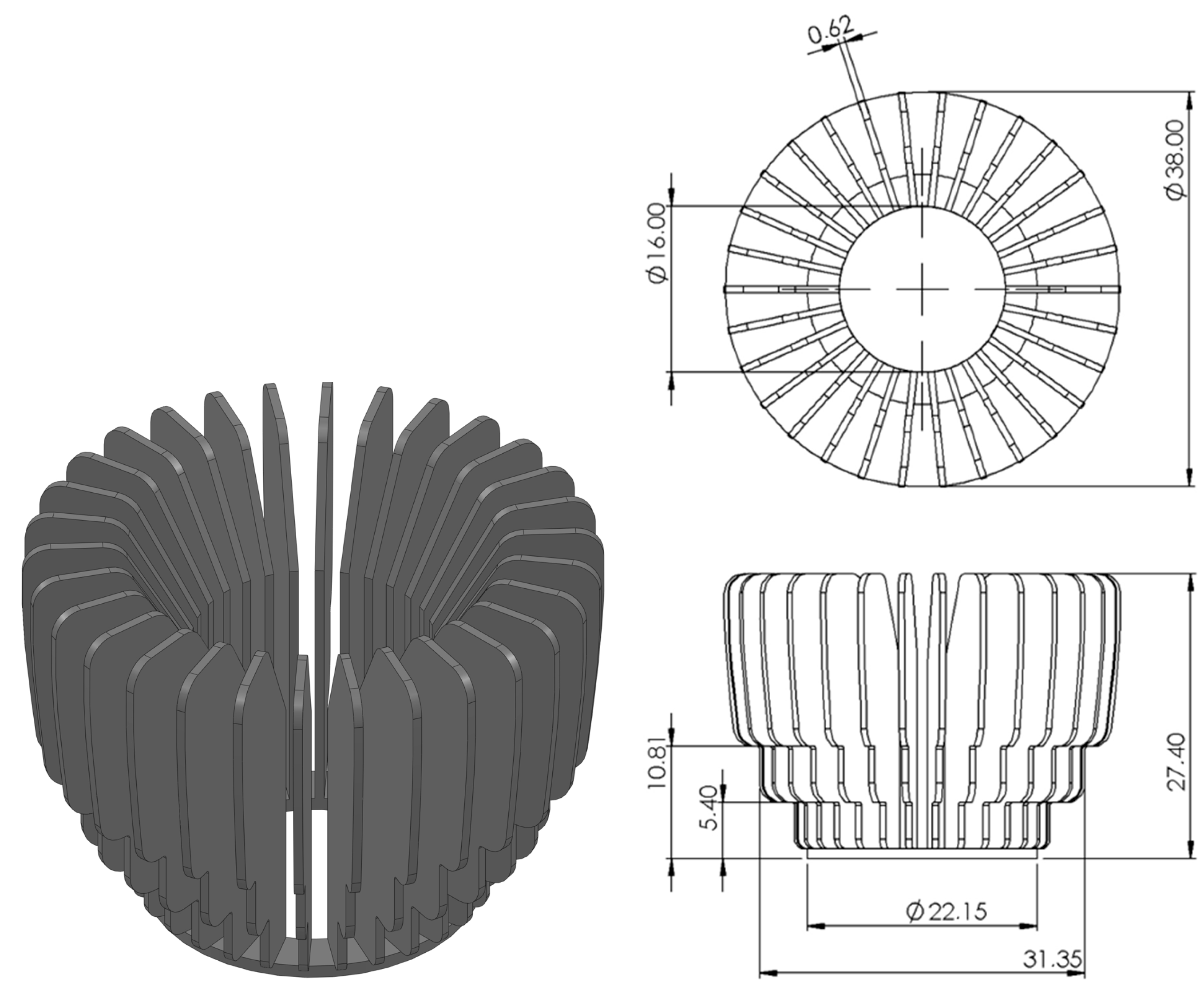
To achieve the goal and solve the problems, a 3D model of the rib design was built in SolidWorks, the geometric features of which are presented in
Figure 3. The version of the software that was used for the computer simulation was SolidWorks Premium 2020 SP2.0.
Computer simulation was carried out using the SolidWorks Flow Simulation Premium add-on, which solves the classical stationary problem of body flow in a channel. Flow Simulation can be used to study flow around objects and to determine the resulting lift and drag forces on the objects due to the flow. We used the method described in the tutorial SolidWorks Flow Simulation [
24]. There, an example of flow modeling is considered to determine the resistance coefficient of a round cylinder immersed in a homogeneous fluid flow. The axis of the cylinder is oriented perpendicular to the flow. Calculations are performed for the range of Reynolds number from 1 to 10
5 [
24]. In our research, fins (
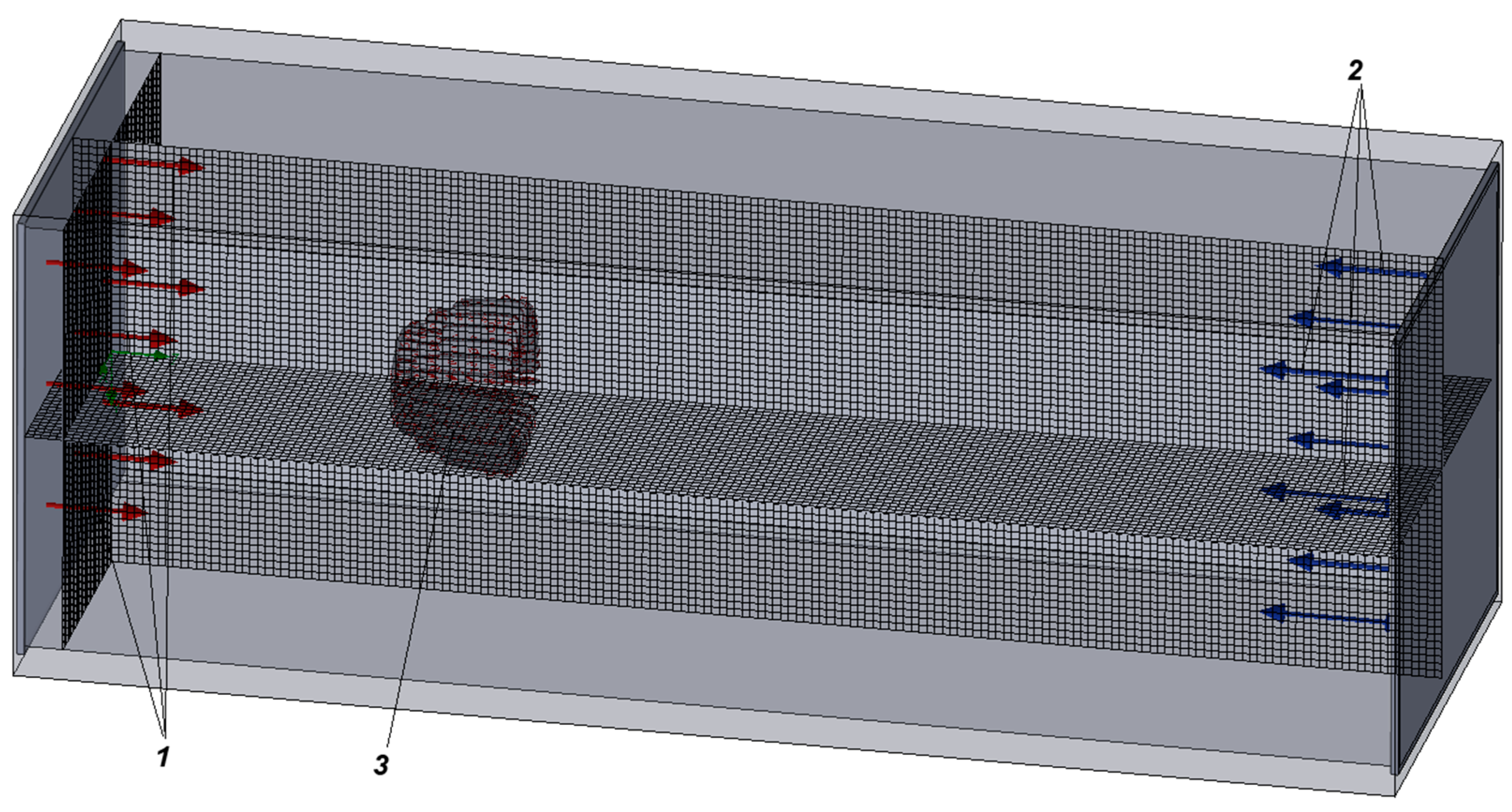
Figure 4) were placed in a rectangular channel with dimensions of 100 mm × 100 mm and a length of 500 mm, while three cases of location were considered. The fins were located in the fluid flow oriented in three different ways: longitudinal flow around the fins from the smaller diameter side; longitudinal flow around the ribbing from the side of the larger diameter; and transverse flow of fins.
For the simulation, we chose to use the default configurations, chose SI as the unit system, and chose the analysis type Internal. The Internal problem was set, without heat exchange with ideal walls. From the menu for gases, “Air” was selected and added to the list of liquids in the project. Thermophysical properties of air are taken from the built-in library SolidWorks Premium 2020 at a temperature of t = 20 °C. A goal was added to find the force in the direction of the axis Z. In addition, a goal was added to the equation using the “insert equation goal” to find the drag coefficient. To implement the finite element method, the design areas are divided into elements of the main determining dimensions using the module Mesh (
Figure 4). SolidWorks Flow Simulation technology uses Cartesian-based meshes for CAD-embedded CFD, where meshes play a key role. Through this approach, cells are fully within solid bodies (solid cells), in the fluid (fluid cells), or intersecting the immersed boundary (termed “partial cells”). A partial cell consists of two control volumes: one fluid CV and one solid CV, each fully within a solid or fluid. Geometric parameters, such as volume and cell center coordinates, are calculated for each CV. Additionally, data on areas and normal vector direction for bounding faces are obtained from the native CAD model. This enables detailed specification of geometry aspects within partial cells, such as solid edges. The Grid Setup Options that are applied follow [
24,
25,
26]. The division into finite elements is performed by the “Mesh” operation, the quality of the mesh is “medium”, and the basic element is tetrahedron with the size 2.8⸱× 10
−5 m. When constructing a grid, the function is included «Use Adaptive Sizing» setting the parameter «Resolution» equal to 6.
Boundary conditions:
Air velocity at the inlet: boundary type “inlet velocity”; boundary conditions: velocity in range from 0.1 m/s to 6 m/s; size 100 mm × 100 mm (
Figure 4, position 1).
Ambient pressure from the channel: boundary type “outlet pressure”; boundary conditions: static pressure 101,300 Pa; size 100 mm × 100 mm (
Figure 4, position 2).
The surface of the ribbing: boundary type “ideal wall”, smooth without roughness and without slipping; area 8172.23 mm
2 (
Figure 4, position 3).
Research was conducted for the range of velocities from 0.1 m/s to 6 m/s, which for this channel corresponds to a change in Reynolds number from 400 to 30,000. For higher velocities and, accordingly, Reynolds numbers, no research was conducted, since the operating speed in industrial heat exchange equipment rarely exceeds 10 m/s. In the case of numerical modelling at values higher than 7 m/s, there is a need to change the calculation model from I-L to k-epsilon, which will make it impossible to compare the results. To solve the problem, model I-L (inviscid–laminar) was chosen, which is used in the case of low-viscosity liquids. Experience shows, however, that when some bodies flow around a low-viscosity fluid (such as water, air), braking due to viscous friction covers only a thin wall layer. Beyond this layer, viscosity has a negligible effect on the distribution of velocities and pressures. Therefore, to study external flow, it is possible to use methods of ideal fluid dynamics, which significantly simplifies the problem compared to the dynamics of a viscous fluid. Neglecting viscosity also helps solve one-dimensional flow problems as a first approximation. Inviscid analysis neglects the effect of viscosity on the flow and is appropriate for high Reynolds number applications where inertial forces dominate the viscous forces. In this simulation, the velocity is high and we can assume it to be inviscid. In general, the flow of an incompressible fluid can be described by the Navier–Stokes equation [
27]:
where
ρ—density of the coolant, [kg/m
3];
Dυ/Dt—rate of change of fluid velocity at a point;
∇P—part responsible for the pressure exerted on the particle;
μ∇2υ—part responsible for the viscosity of the liquid;
f—external forces that we apply to a fluid.
When viscous forces are neglected, such as in the case of inviscid flow, the Navier–Stokes equation can be simplified to a form known as the Euler equation. This simplified equation is applicable to inviscid flow as well as flow with low viscosity and a Reynolds number much greater than one [
27].
where
ρ—density of the coolant, [kg/m
3];
Dυ/Dt—rate of change of fluid velocity at a point;
∇P—part responsible for the pressure exerted on the particle;
f—external forces that we apply to a fluid.
The results were obtained for different variables: flow rate, total pressure, dynamic pressure, and turbulence energy. For each experiment, the value of Δ
P was determined—the pressure difference before and after finning and the value of the dynamic pressure (
ρ⸱
υ2)/2 (the value was taken as the average for the channel section at a distance of up to 2 cm before the fin and 5 cm behind it). The ratio of these two values is the value of the drag coefficient:
In this way, an array of values of drag coefficients was obtained for three different variants of the location of the fins in the air flow at different Reynolds numbers. In the framework of this study, the mode of motion was determined by the Reynolds number, where Re < 2300 is a laminar mode, 2300 < Re < 10,000 is a transitional mode, and Re > 10,000 is a turbulent mode.
To ensure the convergence of the calculation, a convergence goal was automatically set for the Total Pressure with a criterion of 4.1 Pa. The target of convergence was reached in 155 iterations, after which the results were obtained.
4. Validation
Solution verification is a very important step in FEM modelling research. To verify the results, it is necessary to compare the actual simulation model with certain and correct results. The peculiarity of the geometry of the objects under study in our work requires a search for scientific works on similar geometric shapes. However, there are practically no works devoted to the aerodynamics of single-finned nozzles, with the exception of studies of the aerodynamic resistance of a bundle of finned heater tubes. For this reason, we had to look for papers that conduct similar studies for similar geometries. An article devoted to the study of the drag coefficients of bullets for air rifles with a wide range of geometries provides a table of coefficient values for 30 typical bullet geometries for air guns. In particular, the drag coefficient for each bullet using 4.5 mm caliber bullets was tested at Ma ~ 0.57, Re ~56,000 and 5.5 mm caliber bullets at Ma ~ 0.57, Re ~ 68,000, and the effect on the coefficient aerodynamic drag of detailed geometries of simple cylinders and cones at the same Mach and Reynolds numbers [
13].
We compared the values of the aerodynamic drag coefficients for shapes close to the geometry of our nozzle, and the values turned out to be very close. Conical shapes with different apex angles (60°, 45°, 30°, 15°, 15° cut cone) lie in the range between
CX = 1.044 and 0.385 [
13]. For 30 bullet shapes with skirts that are close to our geometry, the aerodynamic drag coefficient values are in the range between
CX = 0.358 and 0.777 [
13]. The average value of the drag coefficient for our nozzle with orientation (from smaller to larger diameter) for the turbulent regime is
CX = 0.96.
In addition, based on the graph given by Hoerner for conical bodies, it appears that the drag coefficient is almost linear with a half-peak angle between 0° and 90°. This information makes it possible to obtain an equation that approximates the experimental data for the drag coefficient by the angle of the half apex of the cone [
28]. The given empirical dependence allows you to analytically calculate the resistance coefficient of the conical element depending on the angle
ξ of its semi-vertex:
We used this equation to calculate the drag coefficient; the corresponding angle for our nozzle was chosen to be 60° (for orientation from smaller to larger diameter), resulting in a value of CX = 0.834.
Both verification options provide fairly high convergence, which makes it possible to assert the adequacy of the results obtained.
Mesh independence was verified to ensure the reliability of the simulation results. A series of research tests were conducted for three fin packing orientations to determine the effect of mesh quality on simulation accuracy. Dimensional resolutions from 3 to 7 were used to create the mesh and calculate the drag coefficient. The number of elements in the aerodynamic channel with a finned nozzle for dimensional resolution 6 was 598,792, and for dimensional resolution 7, the number of elements was 1,707,896. The difference in the average aerodynamic drag coefficient between the results for mesh systems with 598,792 and 1,707,896 elements was less than 2% (
Table 1). A further increase in the number of elements is not advisable, since the accuracy of calculations does not increase significantly, and the calculation time increases several times. Therefore, a dimensional resolution of 6 was confirmed and used in this study. The same level of accuracy was obtained for all finned attachment orientations.
5. Results and Discussion
The contour of velocity, pressure, and dynamic pressure are given for three variants of orientation of fins in the channel and for a velocity of 2 m/s. All other values were fixed and entered into the data table, as a result of which a graph was constructed.
Velocity contours during longitudinal and transverse flow around fins are presented in
Figure 5. In case of longitudinal flow, only the plane of the Y–Z contour is shown, since the picture in the X–Z plane at this location is absolutely similar—this is caused by the symmetrical shape of the fins. However, the contours for transverse flow are given for two planes X–Y and X–Z, since in this case, the arrangement of the pattern on the contours is of a different nature and has certain features.
Velocity distribution contours for the placement of transverse flow of fins (
Figure 5d) fully correspond to the results obtained in the study of Filip and Edward Lisowski with the drop-shaped contour of the low pressure zone immediately behind the nozzle and a pressure increase from the upper and lower parts of the fins [
29].
This representation of the results also applies to the value of total pressure (
Figure 6) and dynamic pressure (
Figure 7).
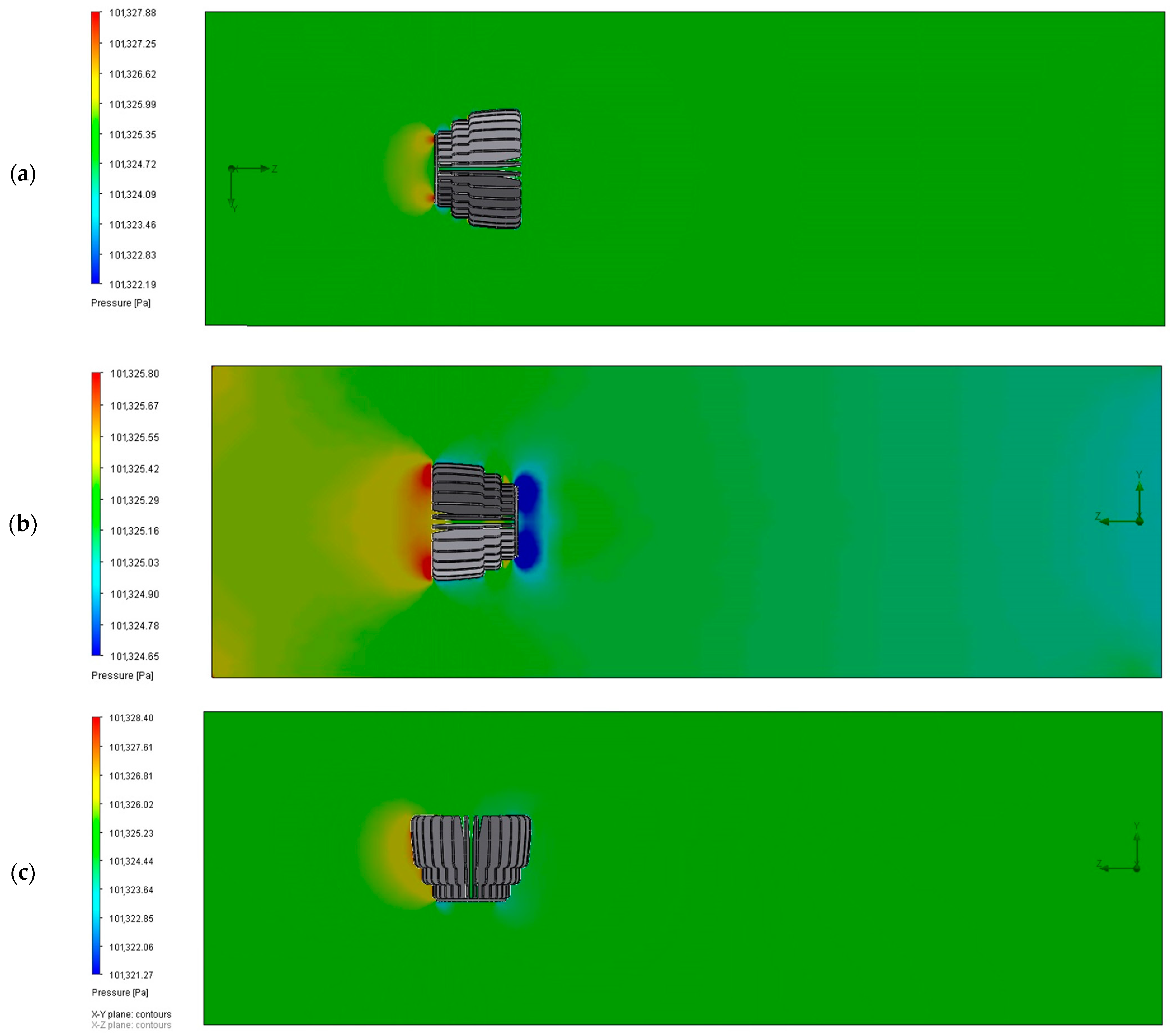
In
Figure 6, the pressure contour during longitudinal and transverse flow around the fins is given.
In
Figure 7, the contour of dynamic pressure (velocity pressure) during longitudinal and transverse flow around the fins is given.
The analysis of the obtained plots allows a qualitative assessment of the character of the aerodynamics of the flow near the fins for three orientations in the channel. In the case of longitudinal flow around the fins with blowing from the smaller diameter side, the maximum velocity values are 2.29 m/s (
Figure 5a), the maximum pressure value is 101,327.6 Pa (
Figure 6a), and the maximum dynamic pressure value (speed pressure) is 3.44 Pa (
Figure 7a).
In the case of longitudinal flow around fins with blowing from the larger diameter side, the maximum velocity values are 2.43 m/s (
Figure 5b), the maximum pressure value is 101,325.8 Pa (
Figure 6b), and the maximum dynamic pressure value (speed pressure) is 3.71 Pa (
Figure 7b).
In the case of transverse flow around the fins, the maximum velocity values are 2.48 m/s (
Figure 5c), the maximum pressure value is 101,327.65 Pa (
Figure 6c), and the maximum dynamic pressure value (velocity pressure) is 3.73 Pa (
Figure 7c).
An important difference between the transverse location of the fins and the longitudinal fins is the difference in the distribution of physical parameters in the main cross-sections, especially the pulsations of velocities and pressures that cause the separation of the flow behind the fins. Turbulence in this case is large-scale, so this orientation of the fins can be considered poorly streamlined. For longitudinal blowing, the geometric shape of the fins is symmetrical, while the ribs are directed in such a way that they form channels that coincide with the direction of the flow and the highly turbulent areas are more local in nature. When comparing the longitudinal orientations, a significant difference in the values of the resistance coefficients was found. The orientation of the fins with flow from a larger diameter to a smaller one is more aerodynamic than the opposite orientation. In our opinion, this is explained by the fact that the flow that hits the ribs is well dissected by it, and the subsequent decrease in diameter contributes to the reduction in turbulence and flow distribution, which positively affects the drag coefficient.
On the basis of numerous simulations, an array of data was obtained and, based on them, a graphical dependence of the Reynolds number on the drag coefficient was constructed, which is presented in
Figure 8.
Analyzing the obtained arrays of values, the following can be noted: the lowest value of the drag coefficient is observed when the fins are oriented in flow from a larger diameter to a smaller one (
Figure 8, red curve 2). The values of the drag coefficient significantly depend on the flow regime. In the laminar flow regime (Re < 2300), the average value of
CX = 1.04, in the transitional flow regime (2300 < Re < 10,000),
CX = 0.74, and in the turbulent regime (Re > 10,000),
CX = 0.22. This case is characterized by a significant decrease in the drag coefficient during the transition from the laminar to the turbulent flow regime; the minimum is observed at the flow speed in the range between 2 and 3 m/s, which corresponds to the range between number Re = 9668 and 14,503, while for the transition from the transitional to the turbulent movement regime, the value is in the range between
CX = 0.18 and 0.14. A further increase in speed leads to a smooth, slight increase in the drag coefficient. This variant of fin orientation can be attributed to a well-streamlined body in which flow separation occurs weakly, which affects small values of the drag coefficient. A different situation is observed with the orientation of the fins in the flow from a smaller diameter to a larger one (
Figure 8, green curve 1). In the laminar mode (Re < 2300), the average value of
CX = 1.74, in the transitional mode (2300 < Re < 10,000),
CX = 1.68, and in the turbulent mode (Re > 10,000),
CX = 0.96. Characteristic for this case of rib orientation are higher values of the drag coefficient than in the previous version, over the entire speed range, although it has a noticeable tendency to decrease with increasing Reynolds numbers. This variant of the orientation of the fins can be attributed to a poorly streamlined body, in which the separation of the flow occurs more pronounced, which affects the higher values of the resistance coefficient.
With the orientation of the fins with transverse flow, the maximum values of the drag coefficient are achieved in the entire range of Reynolds numbers (
Figure 8, purple curve 3). In the laminar mode (Re < 2300), the average value of the aerodynamic resistance coefficient is
CX = 1.74, in the transitional mode (2300 < Re < 10,000),
CX = 1.68, and in the turbulent mode (Re > 10,000),
CX = 0.96. Characteristic of this variant of orientation is a slight change in drag coefficients in different modes of fluid movement. Therefore, for this range of studies, the value of the coefficient can be considered averaged for these modes of movement—
CX = 1.96. This variant of finning can be attributed to bodies with a blunt frontal part, which strongly divides the flow into a zone of high and low pressure, which causes a high coefficient of frontal resistance.
For nozzles with eight ribs in their study, Lisowski obtained the value of the coefficient of aerodynamic drag in CFD modeling—
CX = 1.14 at a speed of 10.03 m/s [
29]. Analyzing the change in the coefficient of aerodynamic drag, according to the graph obtained in our simulation (
Figure 8, curve 3), it can be stated that the drag coefficient at values of the Reynolds number Re > 10,000 tends to decrease. The limiting value in our study corresponds to
CX = 1.83 at 6 m/s, and the reduction in the drag coefficient in the interval 10,000 < Re < 30,000 is 15%. Using the simulation data, it can be assumed that at a speed of 10 m/s, the difference in the coefficients of aerodynamic drag of the fins of our geometry and those studied by Lisowski will not exceed 25%. Such a discrepancy is quite acceptable, since in our study, the nozzle contains thirty ribs, compared to the nozzle with eight ribs in Lisowski’s study [
29]. A denser rib structure can cause an increase in the component of form resistance or friction, which is the result of a higher value of the aerodynamic drag coefficient. However, if our finned nozzle is used as a heat or mass exchange element, then in addition to the coefficient of aerodynamic drag, the developed surface area should be taken into account, which is almost four times greater than the surface of the nozzle in the study by Lisowski [
29].
The obtained values of drag coefficients can be used to carry out estimated aerodynamic calculations of heat exchange elements of a similar geometric configuration. To clarify the obtained values, it is necessary to conduct additional field studies in a wind tunnel, which will be the subject of future research.
6. Conclusions
For the patented design of the fins, a computer simulation was carried out in the SolidWorks Flow Simulation environment, with the coefficients of aerodynamic resistance determined for three variants of its location in the flow. The averaged values are given in the work and allow estimation of the influence of the orientation of the fins on the aerodynamic resistance.
The analysis of the simulation results made it possible to classify the fins and assign them to bodies with poor flow, which is expressed in high values of the frontal drag coefficient CX. An exception is the situation with orientation in flow from a larger diameter to a smaller one for the turbulent flow regime, in which a drop in the value of the drag co-efficient is observed.
The lowest value of the drag coefficient is observed when the fins are oriented from a larger diameter to a smaller one. In the laminar regime (Re < 2300), the average value of CX = 1.04, in the transitional regime (2300 < Re < 10,000), CX = 0.74, and in the turbulent regime (Re > 10,000), CX = 0.22.
The research allows us to conclude that, in practice, during the design of heat exchange elements, it is rational to use fins of the proposed geometry by orienting them in the flow of the coolant exclusively from a larger to a smaller diameter. This orientation of the fins gives the lowest values of the drag coefficient over the entire range of Reynolds numbers.
The results of this study will be useful for researchers and engineers who design a heat exchanger in which finned tubular elements are use, e.g., radiators of cooling systems for computer chips and processors and devices in which advanced heat and mass exchange surfaces are used as regular nozzles (scrubbers, absorbers, and bioreactors).


