Article

Predictive Modeling of Light–Matter Interaction in One Dimension: A Dynamic Deep Learning Approach

by
Özüm Emre Aşırım
1,*,
Ece Z. Asirim
2,* and
Mustafa Kuzuoğlu
3
1
TUM School of Computation, Information and Technology, Technical University of Munich, Hans-Piloty-Str. 1, 85748 Garching, Germany
2
Department of Informatics, University of Zurich, Binzmühlestrasse 14, CH-8050 Zurich, Switzerland
3
Department of Electrical and Electronics Engineering, Middle East Technical University, 06800 Ankara, Turkey
*
Authors to whom correspondence should be addressed.
Appl. Syst. Innov. 2024, 7(1), 4; https://doi.org/10.3390/asi7010004
Submission received: 27 October 2023 / Revised: 24 November 2023 / Accepted: 20 December 2023 / Published: 25 December 2023
(This article belongs to the Section Applied Mathematics)

Abstract

:
The mathematical modeling and the associated numerical simulation of the light–matter interaction (LMI) process are well-known to be quite complicated, particularly for media where several electronic transitions take place under electromagnetic excitation. As a result, numerical simulations of typical LMI processes usually require a high computational cost due to the involvement of a large number of coupled differential equations modeling electron and photon behavior. In this paper, we model the general LMI process involving an electromagnetic interaction medium and optical (light) excitation in one dimension (1D) via the use of a dynamic deep learning algorithm where the neural network coefficients can precisely adapt themselves based on the past values of the coefficients of adjacent layers even under the availability of very limited data. Due to the high computational cost of LMI simulations, simulation data are usually only available for short durations. Our aim here is to implement an adaptive deep learning-based model of the LMI process in 1D based on available temporal data so that the electromagnetic features of LMI simulations can be quickly decrypted by the evolving network coefficients, facilitating self-learning. This enables accurate prediction and acceleration of LMI simulations that can run for much longer durations via the reduction in the cost of computation through the elimination of the requirement for the simultaneous computation and discretization of a large set of coupled differential equations at each simulation step. Our analyses show that the LMI process can be efficiently decrypted using dynamic deep learning with less than 1% relative error (RE), enabling the extension of LMI simulations using simple artificial neural networks.

1. Introduction

Modeling the behavior of electromagnetic waves in free space and also in complex media is well-known to be an involved procedure that requires the concurrent solution of Maxwell’s equations with the Schrödinger wave equation in order to fully capture the wave behavior under time-varying electron dynamics [1,2,3,4]. Various computational methods, such as the Finite-Difference Time-Domain (FDTD) Method, Finite Element Method, Method of Moments, Discontinuous Galerkin Method, etc., have been proposed for solving the Maxwell equations in simple and complex media [5,6,7]. These methods vary in their success in capturing electromagnetic wave behavior in spatial and temporal domains through media that are simple and complex (bi-anisotropic, in-homogenous, nonlinear, etc.).
Under an interaction medium with slowly varying electron dynamics, solving the Maxwell equation is usually sufficient, in which case the electron dynamics can be modeled using the rate equations. The most commonly used method for dealing with complex media in microwave theory, optics, and photonics is the FDTD method. The FDTD method, besides being theoretically simple, is straightforward to implement computationally and can be applied to model wave dynamics in almost all kinds of complex media [5]. However, the FDTD method is limited in its ability to model geometrically complex media or media with rough surfaces and significant shape irregularities. In this study, we will focus on using the FDTD method for modeling the light–matter interaction (LMI) process in nonlinear dispersive media, typically encountered in optics/photonics.
To model the behavior of light, we use the wave equation derived from Maxwell’s equations by substituting the equation for Ampere’s law into the equation for Faraday’s law [5,7]. The dynamics of the electrons are accounted for via the polarization term (also involved in the wave equation) [8,9,10,11,12], which is modeled using the Lorentz dispersion equations [5,6]. The wave equation and the Lorentz dispersion equations are coupled to each other through the polarization term [7]. Under a particle-based treatment of the electrons, the electron dynamics are modeled using the rate equations, helping to identify the population of electrons at each energy level in the medium [5]. The set of all coupled differential equations is modeled based on the FDTD discretization. Importantly, the stability of the numerical solutions relies heavily on the preciseness of the spatial and temporal FDTD discretization. If the discretization step size is too large in the temporal domain, then the solutions can become unstable, meaning that the model can produce non-physical values that jump to infinity [5,6,7]. Hence, for the stability of the numerical solutions, it is very important to choose a sufficiently small temporal step size. Note that the temporal step size must be selected in accordance with the spatial step size. This is because one would be interested in capturing every detail of the propagating light wave through the spatial domain of the involved medium, and for that, the spatial step size should be selected as small (how small depends on the medium properties and the desired resolution of the light wave). Once an adequately small spatial step size is determined, the corresponding temporal step size must satisfy the Courant stability criterion, which states that the temporal step size must be smaller than the spatial step size divided by the speed of light c in free space t < x / c [5,6,7]. Given this condition, one is left with the conclusion that in order to simulate and predict the light behavior in complex media with high spatial resolution over a long duration, one must select the temporal and spatial step sizes to be very small, which leads to an enormous computational cost [10,11,12].
Here a major problem occurs because the wavelength of optical waves (mid-infrared–visible–ultraviolet–X-ray) is quite small, often less than 1 µm [13,
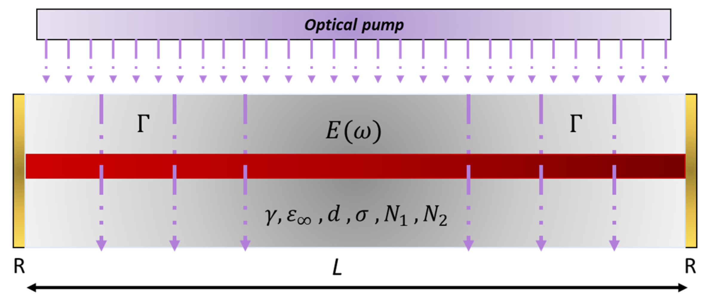
14]. However, many optical phenomena, such as four-wave mixing and parametric amplification, produce a noticeable effect on the macroscale, which is usually much greater than 1 mm. In addition, some optical phenomena, such as interference and laser build-up in a cavity (Figure 1), are only noticeable after relatively long durations (microseconds or milliseconds) [15,16]. In such cases, modeling wave dynamics is a substantial challenge [17,18] which demands the use of supercomputers even under the use of a simple computational algorithm such as FDTD. Therefore, this study aims to come up with a cost-effective alternative solution that extrapolates the solution after a small amount of simulation time.
To achieve this, we resort to deep learning, which can uncover all features of the underlying problem based on a given input-output dataset [19,20,21,22]. Here, we initially define and numerically solve a given problem using the FDTD method under an ultra-fine grid size to ensure stability. Then, for a given input dataset, we achieve an output dataset for a limited simulation duration. We use multilayer perceptrons to form a deep neural network whose coefficients evolve throughout the simulation. After identifying all the coefficients that connect the artificial neurons at each time step, we extrapolate the problem for longer durations by predicting the future values of the network coefficients from their temporal behavior and compare the extrapolated solution with the one that would be attained by running the simulation for the same amount of time for error quantification. Our deep learning model is based on a series of linear-time-invariant (LTI) system expansions that are based on the segmentation of the training data (partitioning of the entire signal data), assuming that the system response changes slowly in time with respect to the period/frequency of the analyzed light wave (which is usually the case in practice) over each of these segments. This is quite accurate because the mathematical model of a multilayer perceptron reduces to multiple LTI system expansions for slowly time-varying systems over segmented training data, where a system can also be approximated as linear [5,6]. Consequently, we use the identified LTI system coefficients at each layer and record their values for all times to extrapolate the wave behavior for longer durations and measure the corresponding extrapolation error by comparing the extrapolated results with the ones obtained via simulation.
Deep learning is based on multilayer neural networks that relate the input data to the output data through a series of coefficient values via inner-product operation [23,24,25,26,27,28,29,30,31,32]. Due to the dramatic increase in the processing power of computers, in the last few decades machine learning has been applied extensively in the field of optics and photonics as it has also been in many other fields [27,28,29]. Over the years, a huge number of papers have focused on machine learning algorithms to uncover hidden physical models in electromagnetics [23,24,25,26,27,28,29]. Notably, research papers that apply machine learning algorithms to predict the nonlinear dynamics of optical systems have received strong attention. These papers have successfully modeled optical systems as robust neural networks that can imitate the behavior of the underlying system with ultimate precision [23,24,25,26,27,28,29,30,31,32]. A striking observation in many of these papers is that the concern is to identify the originally unknown system within the duration of the performed experiments with no extrapolation of the system coefficients for predicting future system behavior. This is problematic because the input signal characteristics often change, leading to a response that differs from the trained model. This unpredictability forms the core challenge in forecasting system behavior, highlighting a crucial battle between traditional machine learning and advanced deep learning algorithms. Deep learning, distinguished from machine learning by its use of multiple layers, offers a solution to this challenge. Each additional layer in a deep learning model extracts more nuanced features of the underlying system, enhancing the model’s predictive capabilities. Predicting the future weights of each layer enables more accurate predictions of subsequent layers’ weights and, consequently, the future samples of an output dataset. This approach requires the adaptive identification of network coefficients over time, segment by segment, a process we refer to as dynamic deep learning. In this study, we will apply dynamic deep learning to both accelerate and predict complex light–matter interaction (LMI) scenarios where conventional prediction methods fall short, enabling accurate and cost-effective simulations in the field of optics and photonics.

2. Methods

2.1. FDTD-Based LMI Model Based on Two Energy Levels

We first investigate the case where photons and electrons interact based on two energy levels with the corresponding frequencies υ 1 and υ 2 . In this case, there are only two transitions, which are 1 2 and 2 1 . Correspondingly, there is only one transition frequency, which is ω R = 2 π ( υ 2 υ 1 ) . Hence, the polarization density goes into resonance only at this frequency. When the interaction material has a single electronic transition frequency, upon excitation of the interaction medium via an optical beam of electric field intensity E, the corresponding wave, polarization, and electron dynamics are modeled as follows [5,6,7].
  • Numerical model for wave dynamics (the wave equation):
2 E μ 0 ε 2 E t 2 = μ 0 σ E t + μ 0 d 2 P d t 2    
  • Numerical model for polarization dynamics (Lorentz dispersion eq. up to the 3rd order):
d 2 P d t 2 + γ R d P d t + ω R 2 P ω R 2 P 2 2 ( N 1 N 2 ) e d + ω R 2 P 3 6 ( N 1 N 2 ) 2 e 2 d 2 = ( N 1 N 2 ) e 2 E m e
  • Numerical model for electron dynamics:
d N 1 d t = Γ N 1 + N 2 τ 21 1 ( h / 2 π ) ω R E d P d t  
d N 2 d t = Γ N 1 + 1 ( h / 2 π ) ω R E d P d t N 2 τ 21    
E: Electric field, μ0: Free space permeability, ε: Background permittivity, t: Time, h: Planck constant, σ: Conductivity, P: Polarization density, γR: Polarization damping rate, ωR: Angular resonance frequency, N1: Electron density at the first level, N2: Electron density at the second level, τ21: Transition lifetime (level 2 to level 1), d: Atom diameter, me: Electron mass, e: Elementary charge, and Γ: Electron pump rate.
Here, Equation (1) represents the electric field wave equation for isotropic media that can be easily derived from equations representing Ampere’s Law and Faraday’s Law (also known as Maxwell’s First and Second Equations) [5]. Equation (2) is the famous Lorentz dispersion equation, which governs the temporal behavior of the polarization density of bound electrons under electric field excitation. The Lorentz dispersion equation is analogous to the spring model, which describes the position of a mass that is attached to a spring on which a certain amount of force is exerted. In this case, the electrons are under damped oscillation due to the force that is exerted by the atomic nucleus and the electric field. The damping occurs mainly due to collisions with other electrons. Equations (3) and (4) represent the electron populations at level 1 (ground level) and level 2 (excited level). Since the polarization density in Equation (2) is created by the electron population difference between level 1 and level 2, and since the electric field intensity in Equation (1) depends on the polarization density (which is the source term), Equations (1)–(4) are coupled to each other and must be solved simultaneously. The situation is more complicated in an interaction medium with more energy levels (see next section).

2.2. FDTD-Based LMI Model Based on Three Energy Levels

If there are three energy levels involved in the electron/photon dynamics, then the interaction medium can have six different electron transitions 1 2 ,   1 3 ,   2 3 and three electron transition frequencies ( υ 3 > υ 2 > υ 1 ,   ω 1 = 2 π ( υ 2 υ 1 ) , ω 2 = 2 π ( υ 3 υ 1 ) , and ω 3 = 2 π ( υ 3 υ 2 ) ). In this case, the associated LMI process is governed by modified versions of Equations (1)–(4), which are given as follows:
  • Numerical model for wave dynamics:
    2 E μ 0 ε 2 E t 2 = μ 0 σ E t + μ 0 d 2 P 1 + P 2 + P 3 d t 2    
  • Numerical model for polarization dynamics:
d 2 P 1 d t 2 + γ 1 d P 1 d t + ω 1 2 P 1 ω 1 2 P 1 2 2 ( N 1 N 2 ) e d + ω 1 2 P 1 3 6 ( N 1 N 2 ) 2 e 2 d 2 = ( N 1 N 2 ) e 2 E m e
d 2 P 2 d t 2 + γ 2 d P 2 d t + ω 2 2 P 2 ω 2 2 P 2 2 2 ( N 1 N 3 ) e d + ω 2 2 P 2 3 6 ( N 1 N 3 ) 2 e 2 d 2 = ( N 1 N 3 ) e 2 E m e
d 2 P 3 d t 2 + γ 3 d P 3 d t + ω 3 2 P 3 ω 3 2 P 3 2 2 ( N 2 N 3 ) e d + ω 3 2 P 3 3 6 ( N 2 N 3 ) 2 e 2 d 2 = ( N 2 N 3 ) e 2 E m e
  • Numerical model for electron dynamics:
d N 1 d t = Γ N 1 + N 2 τ 21 + N 3 τ 31 1 ( h / 2 π ) ω 1 E d P 1 d t 1 ( h / 2 π ) ω 2 E d P 2 d t ,           ( Γ = Γ 1 + Γ 2 )  
d N 2 d t = Γ 1 N 1 + 1 ( h / 2 π ) ω 1 E d P 1 d t N 2 τ 21 + N 3 τ 32
d N 3 d t = Γ 2 N 1 + 1 ( h / 2 π ) ω 2 E d P 2 d t N 3 τ 31 N 3 τ 32
Notice that in this case, the electric field wave equation (Equation (5)) is stimulated by three different polarization terms ( P 1 ,   P 2 ,   P 3 ) which are governed by Equations (6)–(8), representing the dynamics of bound charge polarization densities as induced by each electronic transition. The electron populations at each level are modeled via Equations (9)–(11), which are coupled to the Lorentz dispersion equations (Equations (6)–(8)) through the source term and the nonlinear polarization terms. Hence, to solve for the electric field intensity, one must solve all seven equations (Equations (5)–(11)).

2.3. Numerical Discretization

The numerical discretization is carried out in 1D space, considering the case of a single transition based on two-level electron dynamics, using the FDTD method. The discretization for the three-level case is similar and straightforward. Here the electric field and the associated polarization density are discretized in space and time, whereas the electron populations are discretized only in time as it is assumed that the interaction medium is homogenous in density over space. The FDTD discretization of Equations (1)–(4) is carried out as follows [5]:
x : Spatial coordinate , t : Time , E x , t = E i x , j t E i , j ,         i = 1 , 2 , , M i   ,       j = 1 , 2 , , M j E x + x , t E x , t E i + 1 , j E i , j ,       E x , t + t E x , t E i , j + 1 E i , j E x = E i + 1 , j E i 1 , j 2 x , E t = E i , j + 1 E i , j 1 2 t 2 E x 2 = E i + 1 , j 2 E i , j + E i 1 , j x 2 , 2 E t 2 = E i , j + 1 2 E i , j + E i , j 1 t 2 ,
Notice that we are using the central difference approximation for the first derivatives in time and space and applying the standard formulation for the second derivatives.
  • Discretization of the wave equation:
E i , j + 1 = E i + 1 , j 2 t 2 µ 0 x 2 σ t + 2 ε i , j + E i , j 4 µ 0 ε i , j x 2 2 t 2 µ 0 x 2 σ t + 2 ε i , j + E i 1 , j 2 t 2 µ 0 x 2 σ t + 2 ε i , j + E i , j 1 σ t 2 ε i , j σ t + 2 ε i , j 2 σ t + 2 ε i , j P i , j + 1 2 P i , j + P i , j 1
  • Discretization of the Lorentz dispersion equation:
P i , j + 1 = P i , j 1 γ t 2 γ t + 2 + 2 N 1 j N 2 j e 2 t 2 E i , j γ t + 2 m + 2 γ t + 2 { 2 P i , j ω 0 2 t 2 P i , j + ω 0 2 t 2 P 2 i , j N 1 j N 2 j e d ω 0 2 t 2 P 3 i , j N 1 j N 2 j 2 e 2 d 2 }    
  • Discretization of the rate equations:
N 1 j + 1 = N 1 j 1 + 2 t Γ j N 1 j + N 2 j τ 21 2 h ω R E j P j + 1 P j 1
N 2 j + 1 = N 2 j 1 + 2 t Γ j N 1 j N 2 j τ 21 + 2 h ω R E j P j + 1 P j 1
These discretized equations are solved together with the initial and boundary conditions of a given problem, which will be stated in the analyzed cases in Section 3. For the stability of the numerical solutions, the time step t must be chosen to be smaller than the spatial step divided by the speed of light in free space ( t < x / c ) , which is known as the Courant condition [5].

2.4. Multilayer-Perceptron-Based Neural Networks for Modeling 1D Light-Matter Interaction under the Slowly Varying Envelope Approximation

The FDTD simulations generate an output dataset for each input dataset given by the user. To process these input/output datasets for modeling the underlying system, we consider the simplest neural network that can be mathematically expressed through plain matrix multiplication between the network weights and the input data. In matrix notation, the output data y of a single-layer neural network are expressed in terms of the given input data x (we use brackets for representing network weights and parenthesis for input/output data).
y 1 . y n = L 1 w 1 1 ; 1 w 1 1 ; K 1 w 1 n ; 1 w 1 n ; K 1 x 1 . x K 1
y = L 1 { w 1 x }
y = y 1 , y 2 , , y n ,     x = x 1 , x 2 , , x n
where w 1 is the coefficient matrix containing the weights that connect/relate the network nodes, and the activation operator L 1 can be either a linear or a nonlinear operator that transforms the elements of the result vector of the matrix multiplication to fit within a certain range in accordance with the analyzed problem and the underlying system.
For a given output sample y n , Equation (16) can also be expressed via the following summation term:
y n = L 1 k = 1 K 1 w 1 n ; k x ( k )
In system theory, Equation (17) represents the response of a nonlinear time-varying (NTV) system [33,34]. For slowly (time) varying systems, an NTV system can be approximated as a linear time-invariant (LTI) system within narrow time intervals, in which case Equation (17) can be expressed by the time shift between the input and output samples in the form of a convolution operation [34]:
y n = L 1 k = 1 K 1 w 1 k x ( n k ) = L 1 k = 1 K 1 w 1 n k x ( k ) ,     n > K 1
which can be rewritten as a matrix equation ( L 1 is now an identity operator):
y K 1 + 1 . y n = L 1 w 1 K 1 w 1 1 w 1 n 1 w 1 n K 1 x 1 . x K 1
Equation (19) has much fewer unknowns to solve for (compared to Equation (16)), as the weight (unknown) matrix can now be vectorized as a time shift vector. For this reason, the LTI system approximation provides a great reduction in the computational cost for slowly time-varying systems that are trained gradually over small data segments [35,36,37,38] (see Section 2.5).
In this study, we extend the formulation in Equation (19) for a three-layer neural network, which is considered as a deep learning network with two hidden layers. The use of hidden layers provides more accuracy in determining all features of a given system. In this case, the input–output relationship is modified as follows:
y 1 . y n = L 3 w 3 1 ; 1 w 3 1 ; K 3 w 3 n ; 1 w 3 n ; K 3 L 2 w 2 1 ; 1 w 2 1 ; K 2 w 2 K 3 ; 1 w 2 K 3 ; K 2 L 1 w 1 1 ; 1 w 1 1 ; K 1 w 1 K 2 ; 1 w 1 K 2 ; K 1 x 1 . x K 1
Based on Equation (20), one can deduce that each output sample is related to the input samples through the following mathematical relation:
y n = L 3 k = 1 K 3 w 3 n ; k L 2 l = 1 K 2 w 2 k ; l L 1 q = 1 K 1 w 1 l ; m x ( m )
Just as in the case for a single-layer network, assuming a slowly time-varying system and using small segments of training data, Equation (21) can be expressed in terms of the time shift between the input and output samples over each given training segment (LTI system approximation), which is represented as a serial convolution operation between the network weights and the input data:
y n = k = 1 K 3 l = 1 K 2 m = 1 K 1 w 3 [ n k ] w 2 k l w 1 l m x ( m )
in which case the activation functions are identity operators. In this study, we will base our approach on Equation (22) to train a 3-layer network for identifying the systems that govern an LMI process.

2.5. Segmentation of a Given Input/Output Dataset for Neural Network Training

In order to evaluate the weights of the three-layer neural network adaptively using many narrow time intervals, one has to divide a given signal into many small segments, each containing M samples that can be used to train the neural network for identifying the local behavior of the underlying system. Each segment should be small compared to the size of the entire signal so that both the linearity and the slowly time-varying system approximation can be made. By computing the coefficients of a 3-layer network at each and every segment and then combining them, one can determine the temporal evolution of the coefficients (thus the network) through the duration of the entire signal, thereby performing dynamic deep learning that facilitates a self-learning network for precise prediction of future output values even under very limited input data. The segmentation can be performed in different ways, as stated below.
  • Use a segment window of M samples and a segment period of N (N = M) samples:
Under this segmentation, all segments are adjacent to each other and there is no overlap between them. If the entire signal S is divided into P segments, this is stated as follows:
S n ; 1 = s 1 , s 2 , , s M ,       S n ; 2 = s M + 1 , s M + 2 , , s 2 M , , S n ; P = s M × P 1 + 1 , s M × P 1 + 2 , , s M × P    
  • Use a segment window of M samples and a segment period of N (N M) samples:
For this case, the segments may or may not be overlapping depending on N and M:
S n ; 1 = s 1 , s 2 , , s M ,       S n ; 2 = s N + 1 , s N + 2 , , s N + M , , S n ; P = s N × P 1 + 1 , s N × P 1 + 2 , , s N × P 1 + M
If N < M, the overlap ratio is ( M N ) / M . Whereas if N > M, then the overlap ratio is zero. However, if N is much larger than M, then many samples remain idle, which leads to an inefficient use of data. Hence, if no overlap is desired, one should choose N = M.
  • Use a segment window of M samples and a segment period of N (N M) samples:
Here, the overlap ratio is ( M N ) / M 1 . This means that each subsequent segment is nearly identical to its neighbor but not completely the same. This is an efficient use of data in cases where the underlying system is strongly time-variant. Whereas if the system is weakly time-variant, this can cause the unnecessary creation of new segments, which would bring little new information about the system (a slow update of the neural network weights would be sufficient) at the cost of drastically increased computation time.
  • Use a segment window of M samples and a segment period of N = 1 sample:
In this scenario, each consecutive segment differs only through a single sample shift. This means that subsequent segments totally overlap with each other, except for a single sample such that
S n ; i = s M × i 1 , s M × i 1 + 1 , , s M × i 1 , S n ; i + 1 = s M × i 1 + 1 , s M × i 1 + 2 , , s M × i i = 1 , 2 , P               i : S e g m e n t   n u m b e r  
This form of segmentation (Figure 2) enables a very efficient use of data under fast time-variation of the system coefficients. Despite our assumption of a slowly time-varying system, we will make use of this segmentation for a sample-by-sample computation of the neural network coefficients in order to see their temporal evolution in full resolution.
Under such sample-by-sample segmentation, to predict the upcoming samples of the output vector y, one has to solve for the set of coefficients at each layer and for each estimated sample. This means that to predict N future samples, the coefficient vectors w 1 , w 2 , w 3 must be solved based on Equation (22), which can be expanded as three consecutive matrix multiplications:
y M + 1 . y M + N = w 3 1 w 3 K 3 w 3 N w 3 N K 3 + 1 z M . z M K 3 + 1
z M K 3 + 1 . z M = w 2 1 w 2 K 2 w 2 K 3 w 2 K 3 K 2 q M K 3 . q M K 3 K 2 + 1
q M K 3 K 2 + 1 . q M K 3 = w 1 1 w 1 K 1 w 1 K 2 w 1 K 2 K 1 x M K 3 K 2 . x M K 3 K 2 K 1 + 1          
where x is the input vector and {q, z} are intermediate outputs that ultimately yield the output vector y. Simplified forms of Equations (26)–(29) will be referred to for carrying out the dynamic coefficient (system) identification procedures in the next section based on the least-squares method, using sample-by-sample segmentation under the use of linear operators. Note that Equations (26)–(28) imply M K 3 + K 2 + K 1 ,   K 3 > K 2 ,     a n d   K 2 > K 1 .

2.6. Training of the Multilayer Perceptron over Each Data Segment Based on Output Data

The system coefficients can be evaluated solely based on past samples of the output data y . Hence, one does not necessarily need the input data to perform a prediction. Also, one can simply use Equation (22) over each training segment where nonlinear operators are not required due to the limited size of the involved segment. By re-labeling the coefficients as a, b, and c, Equation (22) can be rewritten as follows (note that x[m] is replaced with y[m] as past samples of the output data are considered input signal samples in the case of prediction):
y n = k = n K 3 n 1 a [ n k ] l = k K 2 k 1 b k l m = l K 1 l 1 c l m y ( m ) ,     n > k
Using the following operational tricks, Equation (29) can be converted into Equation (36):
y n = k = n K 3 n 1 a [ n k ] z ( k ) = k = n K 3 n 1 a [ k ] z ( n k )
y n = k = 1 K 3 a [ k ] l = n k 1 n k K 2 b n k l m = 1 K 1 c m y ( l m )
l   n k l
y n = k = 1 K 3 a [ k ] l = 1 K 2 b l m = 1 K 1 c m y ( n k l m )
k   k l
y n = k = l + 1 l + K 3 a [ k l ] l = 1 K 2 b l m = 1 K 1 c m y ( n k m )
l   l m
y n = k = l m + 1 l m + K 3 a [ k l + m ] l = m + 1 m + K 2 b l m m = 1 K 1 c m y ( n k m )
k   k m
y n = k = l + 1 l + K 3 a [ k l ] l = m + 1 m + K 2 b l m m = 1 K 1 c m y ( n k )
y n = k = l + 1 l + K 3 l = m + 1 m + K 2 m = 1 K 1 c m b l m a k l y ( n k )
The good thing about Equation (36) is that it can be nicely decoupled into the following three equations:
y n = k = 1 K 3 a k y ( n k )
a k = l = 1 K 2 b l a k l
b l = m = 1 K 1 c m b l m                
where the output signal can be directly expressed in terms of its past values in a single equation.
Equations (37)–(39) can be rewritten using matrix equations that describe the prediction of N upcoming samples based on the past M samples (segmental training data):
y M + 1 . y M + N = y M y M + 1 K 3 y M + N 1 y M + N K 3 a [ 1 ] . a [ K 3 ]
a [ K 2 + 1 ] . a [ K 3 ] = a K 2 a 1 a K 3 1 a K 3 K 2 b [ 1 ] . b [ K 2 ]          
b [ K 1 + 1 ] . b [ K 2 ] = b K 1 b 1 b K 2 1 b K 2 K 1 c [ 1 ] . c [ K 1 ]          
Using Equation (40), one can solve for the set of K 3 coefficients for the first layer via the least-squares method. The same goes for the second- and third-layer coefficients. The coefficient matrices always depend on the past values of the coefficients of the previous layer ( K 2 coefficients for the second layer and K 1 coefficients for the first layer). Once all the coefficients for each layer are solved, future samples of y(n) can be predicted using sequential matrix updates and multiplication. However, Equations (40)–(42) do not yield the time-dependent values of the coefficients, which prevents the prediction of future values of the coefficients and hinders the adaptive prediction of future output samples. For a self-learning or self-adaptive neural network, the coefficients must evolve with each and every new sample so that the future values of the coefficients can also be predicted from their time series, enabling more accurate output signal prediction under the limited availability of input data. This enables a dynamic evolution of multilayer perceptrons through segmental training where each segment differs only via a single sample shift so that the coefficients are instantly adapted for an “infinitesimal” (unit sample) change. To attain the matrices that contain the time variation (past values) of the coefficients, every set of coefficients needs to be solved per new sample. Therefore, over each segment, the training of the network should be carried out as follows:
y n T M . y n T 1 = y n T M 1 y n T M K 3 y n T 2 y n T K 3 1 a 1 n T 1 . a K 3 n T 1
a 1 n T 1 . a K 3 n T 1 = a 1 n T 2 a 1 n T K 2 1 a K 3 n T 2 a K 3 n T K 2 1 b 1 n T 1 . b K 2 n T 1
b 1 n T 1 . b K 2 n T 1 = b 1 n T 2 b 1 n T K 1 1 b K 2 n T 2 b K 2 n T K 1 1 c 1 n T 1 . c K 1 n T 1
n : S a m p l e   n u m b e r ,   M : S e g m e n t   s i z e ,   T : T i m e   s h i f t ,     T = 1 , 2 , 3 , 4 , , L M
Using Equations (43)–(45), one can perform an adaptive prediction at every instantaneous sample of the output signal based on the 3-layer network. This requires the instantaneous solution of each set of coefficients through the least-squares method, as follows:
y = Y T a ,     a = A T b ,     b = B T c ,           A ,   B ,   Y : C o e f f i c i e n t   m a t r i c e s
a = ( Y T Y ) 1 Y T y ,     b = ( A T A ) 1 A T a ,     c = ( B T B ) 1 B T B              
Therefore, once the coefficients over a certain segment are identified, the future samples of the output signal y can be predicted via Equation (48):
y = Y T A T B T c = B A Y T c    
Note that the coefficient matrices are constructed from past samples of the coefficients themselves. Hence, once a certain coefficient vector (a, b) is solved, its coefficient matrix (A, B) is known, which enables the prediction in Equation (48).

3. Results

3.1. Frequency Generation via Optical Wave Mixing in a Micro-Resonator

3.1.1. Difference Frequency Generation Process

The first optical process that we model using a three-layer network is the difference frequency generation process, which is a nonlinear process that occurs when two high-amplitude waves E 1 and E 2 are simultaneously fed into a cavity. Here, the cavity is composed of two perfectly reflective walls and a Gallium–Arsenide interaction medium that is inserted between the cavity walls. The excited waves are given as follows:
E 1 x = 0   μ m , t = 0   s = 4 × 10 8 × sin 2 π 2.5 × 10 14 t   V / m           ( I n f r a r e d   w a v e   a t   250   T H z ) E 2 x = 0   μ m , t = 0   s = 3 × 10 8 × sin 2 π 1.5 × 10 14 t   V / m           ( I n f r a r e d   w a v e   a t   150   T H z )
Hence, the total excitation wave at t = 0 s is given as follows:
E t o t a l x = 0   μ m , t = 0   s = 4 × 10 8 × sin 2 π 2.5 × 10 14 t V / m + 3 × 10 8 × sin 2 π 1.5 × 10 14 t   V / m
The simulation setting and the properties of the interaction medium are given as follows:
S p a t i a l   a n d   t e m p o r a l   d i s c r e t i z a t i o n :   0 x 5   μ m ,   0 t 5   p s ,   x = 10   n m ,   t = 0.025   f s I n t e r a c t i o n   m e d i u m   r e s o n a n c e   f r e q u e n c y :     f r = 3.45 × 10 14   H z ,       C o n d u c t i v i t y : σ = 10 4   S / m P o l a r i z a t i o n   d a m p i n g   r a t e   o f   t h e   i n t e r a c t i o n   m e d i u m :     γ = 1 × 10 10   H z B a c k g r o u n d   p e r m i t t i v i t y :   ε = 13 ε 0 ,     A t o m i c   d i a m e t e r :   d = 0.3   n a n o m e t e r s ε 0 : F r e e   s p a c e   p e r m i t t i v i t y C a v i t y   r a n g e : 0   μ m < x < 5   μ m ,     E l e c t r o n   d e n s i t y :     N = 1.76 × 10 29 / m 3
As a result of the high optical intensity and the inherent nonlinearity of Gallium–Arsenide atoms, after a certain time, new harmonics will be generated at 100 THz (difference harmonic, mid-infrared) and 400 THz (sum harmonic, red) due to the nonlinear (cross) polarization terms in Equation (2). At the end of the simulation, the final spectrum of the intracavity wave (magnitude of the Fourier transform) is as given in Figure 3.
The modeling of the wave mixing process is computationally costly, and the cost of computation grows exponentially with increasing simulation duration. The efficiency of our three-layer neural network is tested in this case by predicting the temporal behavior of the electric field amplitude of the difference frequency (100 THz) from t = 5 ps to t = 8.5 ps.
The formulations in Equations (43)–(45) are applied with n = 42,500, M = 25,000, K 3 = 4, K 2 = 4, and K 1 = 4 (each layer has four coefficients). Hence, the available training data consist of M = 25,000 samples, and the number of samples to be predicted is 17,500 (n-M). The resulting prediction is shown in Figure 4. In this case, the prediction is highly accurate, with less than 0.08% relative error (RE). A comparison with the theoretical results is also given in Figure 5 regarding the electric field amplitude, based on the given formulation in [39]. The comparison is performed by considering the simulation duration as the total number of roundtrips multiplied by two times the cavity length times the square root of the background permittivity of the medium, divided by the speed of light.
The time variation of the set of four coefficients ( a 1 , a 2 , a 3 , a 4 ) for the first layer of the network is given in Figure 6. Notice that the coefficients are nearly constant as the change in percentage around their mean value is quite insignificant.
The coefficients of the second layer are shown in Figure 7. Compared to the coefficients of the first layer, the percentage of change between the minimum and maximum values of these coefficients is much greater. However, the coefficients of the second layer tend to converge to a certain value after 5 picoseconds, which indicates that the coefficients of the first layer will continue to make the same tiny oscillations around their mean values, indicating that a reliable prediction in the long term is feasible.
Finally, the coefficients of the third layer are given in Figure 8. These coefficients are used to predict whether the convergent behavior of the coefficients of the second layer will persist. There is also a tendency for convergence in this layer, which is easier to spot for the second, third, and fourth coefficients, whereas for the first coefficient, convergence is not that critical as the percentage of change is smaller. Therefore, the third-layer coefficients indicate that the convergence behavior of the second-layer coefficients will persist, which further indicates that the extremely small percentage of change for the first-layer coefficients will continue, enabling one to treat them as constant variables over time and perform a prediction for a duration that is much greater than t = 5 ps.

3.1.2. Sum Frequency Generation Process

As a result of the wave mixing process, the time evolution of the generated electric field of the sum harmonic at 400 THz is illustrated in Figure 9 for both the available data (0 < t < 5 ps) and the predicted data (5 ps < t < 8.5 ps). Expectedly, the electric field of the sum harmonic frequency gradually increases from 0 to 10 9   V/m in 8.5 ps. The available data suggest that the field amplitude reaches 4 × 10 7   V/m in 5 picoseconds, whereas the predicted data show that this amplitude will reach 10 9   V/m in the next 3.5 picoseconds. Due to the nonlinearity of the problem, the time it takes to complete the simulation in 8.5 ps is 3.7 times greater than the time it takes for the simulation to be completed in 5 ps. With the aid of the computed neural network coefficients, the entire process is simulated at a duration that is 100 times smaller. The resulting RE of the prediction is below 0.05% (Equations (43)–(45) are used with n = 42,500, M = 25,000, K 3 = 4, K 2 = 4, and K 1 = 4). A comparison with the theoretical results is given in Figure 10 regarding the electric field amplitude, based on the given formulation in [39] using the same trick as discussed in Section 3.1.1.
The time variation of the set of four coefficients ( a 1 , a 2 , a 3 , a 4 ) for the first layer of the network is given in Figure 11. Just as in the case of difference frequency generation, the coefficients are nearly constant in time, whereas the coefficients of the second layer (see Figure 12) are not constant in time. However, the coefficients of the second layer converge to a constant value over time, indicating that the coefficients of the first layer will behave similarly in the future.
Although it is not as evident as it is for the second-layer coefficients, the coefficients of the third layer also display a convergent behavior (Figure 13), supporting the stability of the second-layer coefficients around their converged value in the long term. The coefficients of the third layer can also be used to verify the convergent behavior of the second-layer coefficients through insertion in the expansion formula in Equation (39).

3.2. Optical Parametric Amplification

Next, we model the optical parametric amplification (OPA) process using our three-layer network model. Here, as opposed to the two previous cases (frequency generation), only one of the waves has a high amplitude, while the other usually has a low amplitude. Through the wave mixing process, over time, the low-amplitude wave draws energy from the cavity that is energized by the high-amplitude wave and becomes amplified while the high-amplitude wave is attenuated. In this case, we consider the amplification of an infrared signal wave at 150 THz using a high-amplitude pump wave at 250 THz. The cavity configuration remains the same as in the previous section. The signal and the pump waves are given as follows (the “signal” and “pump” designations are specific to OPA):
E 1 x = 0   μ m , t = 0   s = 4 × 10 8 × sin 2 π 2.5 × 10 14 t   V / m               ( p u m p   w a v e ) E 2 x = 0   μ m , t = 0   s = 1 × sin 2 π 1.5 × 10 14 t   V / m         ( s i g n a l   w a v e   t o   b e   a m p l i f i e d )
Therefore, the total excitation wave at t = 0 s is given as follows:
E t o t a l x = 0   μ m , t = 0   s = 4 × 10 8 × sin 2 π 2.5 × 10 14 t V / m + 1 × sin 2 π 1.5 × 10 14 t   V / m
The time evolution of the electric field is given in Figure 14 for both the computed and the predicted data. The RE in prediction accuracy was found to be 0.77% in this case. As before, the prediction is performed from t = 5 ps to t = 8.5 ps using the computed data from t = 0 s to t = 5 ps. Once again, the formulations in Equations (43)–(45) are applied with n = 42,500, M = 25,000, K 3 = 4, K 2 = 4, and K 1 = 4. The simulation time using the physical model was 141 s, whereas the computation time is 2.2 s when the derived neural network model is used.
The coefficients of the first layer of the neural network are given in Figure 15. Despite persistent fluctuations, the values of the coefficients are nearly constant over time. The coefficients of the second layer (Figure 16) indicate a convergent behavior, hinting that the temporal behavior of the process is stabilized. The third-layer coefficients (Figure 17) are observed to fluctuate within a narrow range and are stable in their temporal behavior, which hints for a lasting convergence of the second-layer coefficients, implying that the first-layer coefficients will continue to remain (nearly) constant over time.

3.3. Time Evolution of Optical Wave Amplitude in Lossy Micro-Resonators

Optical micro-resonators (or micro-cavities) are often used to confine light waves for sufficiently long durations in order to enable the effective occurrence of certain processes such as parametric amplification, supercontinuum generation, etc. For this reason, the degree of loss in a micro-resonator is of concern as it leads to a decrease in the photon lifetime. In this part, we investigate a lossy optical micro-resonator with an increased interaction medium conductivity and a greater polarization damping rate and predict the overall decay rate for the electric field amplitude within the micro-resonator, for which an analytical expression is not available in the presence of nonlinearity. Here, the total excitation wave at t = 0 s is given as follows:
E t o t a l x = 0   μ m , t = 0   s = 1 × 10 6 × sin 2 π 2.5 × 10 14 t V / m         ( I n f r a r e d   w a v e   a t   250   T H z )
The simulation setting and the properties of the interaction medium are given as follows:
S p a t i a l   a n d   t e m p o r a l   d i s c r e t i z a t i o n :   0 x 5   μ m ,   0 t 5   p s ,     x = 10   n m ,     t = 0.025   f s I n t e r a c t i o n   m e d i u m   r e s o n a n c e   f r e q u e n c y :     f r = 3.45 × 10 14   H z P o l a r i z a t i o n   d a m p i n g   r a t e   o f   t h e   i n t e r a c t i o n   m e d i u m :     γ = 1 × 10 11   H z I n t e r a c t i o n   m e d i u m   c o n d u c t i v i t y :   σ = 10 2   S / m B a c k g r o u n d   p e r m i t t i v i t y :   ε = 13 ε 0 ,     A t o m i c   d i a m e t e r :   d = 0.3   n a n o m e t e r s C a v i t y   r a n g e : 0   μ m < x < 5   μ m ,     E l e c t r o n   d e n s i t y :     N = 1.76 × 10 29 / m 3
For the sake of simplicity, the walls of the micro-cavity are assumed to be perfectly reflective, so the cavity loss is solely due to the dielectric and conduction losses in the interaction medium. The resulting computed and predicted data are shown in Figure 18. Using a three-layer neural network (Equations (43)–(45) are used with n = 65,000, M = 25,000, K 3 = 16, K 2 = 16, and K 1 = 16) with 16 coefficients at each layer, it is successfully (RE: 0.94%) predicted that the electric field amplitude in the micro-cavity will decrease by 12% within 13 picoseconds, which enables an estimation of the total decay rate in the cavity.
The time variation of the first-, second-, and third-layer coefficients are given in Figure 19, Figure 20 and Figure 21, respectively. Compared to the previously analyzed cases, the coefficients for each layer are more fluctuating due to the dominance of the interference effect in the cavity.

4. Conclusions

The light–matter interaction (LMI) process can be accurately decrypted using a three-layer neural network that can be trained during the simulation of a given LMI process that is based on the actual physical model. The network coefficients are dynamically evaluated over many consecutive segments of the available simulation data (each consecutive segment differs only by a sample shift), and their corresponding time evolution can be attained by recording their values for each segment. Based on the time evolution of the network coefficients of the second and third layers, the upcoming values of the first layer can be predicted, which can be used to extrapolate the future values of the output signal. The extrapolation can be made simply through a convolution operation between the network weights and the past values of the output data since the training of the network is performed in a piecewise manner through segmentation, where a linearization approximation can be made. Our computations show that the extrapolation error is quite low for the predicted part of the electric field (light) amplitude, which suggests that the use of a well-trained adaptive neural network can drastically reduce the computation time for the optical electric field and can be used to accelerate long simulations in optics and photonics for modeling scenarios where ultra-fine spatial and/or temporal grid-size is required.

Author Contributions

Conceptualization, Ö.E.A.; methodology, Ö.E.A.; software, Ö.E.A. and E.Z.A.; validation, Ö.E.A.; formal analysis, Ö.E.A.; investigation, Ö.E.A.; resources, Ö.E.A. and E.Z.A.; data curation, Ö.E.A.; writing—original draft preparation, Ö.E.A.; writing—review and editing, Ö.E.A. and E.Z.A.; visualization, Ö.E.A. and E.Z.A.; supervision, M.K. All authors have read and agreed to the published version of the manuscript.

Funding

This research received no external funding.

Institutional Review Board Statement

Not applicable.

Data Availability Statement

Data is contained within the article.

Conflicts of Interest

The authors declare no conflicts of interest.

References

  1. Genty, G.; Salmela, L.; Dudley, J.M.; Brunner, D.; Kokhanovskiy, A.; Kobtsev, S.; Turitsyn, S.K. Machine learning and applications in ultrafast photonics. Nat. Photonics 2021, 15, 91–101. [Google Scholar] [CrossRef]
  2. Hughes, T.W.; Minkov, M.; Williamson, I.A.D.; Fan, S. Adjoint method and inverse design for nonlinear nanophotonic devices. ACS Photonics 2018, 5, 4781–4787. [Google Scholar] [CrossRef]
  3. Närhi, M.; Salmela, L.; Toivonen, J.; Billet, C.; Dudley, J.M.; Genty, G. Machine learning analysis of extreme events in optical fibre modulation instability. Nat. Commun. 2018, 9, 4923. [Google Scholar] [CrossRef] [PubMed]
  4. Raissi, M. Deep hidden physics models: Deep learning of nonlinear partial differential equations. J. Mach. Learn. Res. 2018, 19, 932–955. [Google Scholar]
  5. Taflove, A.; Hagness, S. Computational Electrodynamics: The Finite-Difference Time-Domain Method, 3rd ed.; Artech House: Nowood, MA, USA, 2005; pp. 353–383. [Google Scholar]
  6. Aşırım, Ö. Far-IR to deep-UV adaptive supercontinuum generation using semiconductor nano-antennas via carrier injection rate modulation. Appl. Nanosci. 2021, 12, 1–16. [Google Scholar] [CrossRef]
  7. Aşırım, Ö.; Kuzuoğlu, M. Super-Gain Optical Parametric Amplification in Dielectric Micro-Resonators via BFGS Algorithm-Based Non-Linear Programming. Appl. Sci. 2020, 10, 1770. [Google Scholar] [CrossRef]
  8. Peter, R.W.; Arbouet, A.; Girard, C.; Muskens, O.L. Deep learning in nano-photonics: Inverse design and beyond. Photonics Res. 2021, 9, B182–B200. [Google Scholar]
  9. Alagappan, G.; Ong, J.R.; Yang, Z.; Ang, T.Y.L.; Zhao, W.; Jiang, Y.; Zhang, W.; Png, C.E. Leveraging AI in Photonics and Beyond. Photonics 2022, 9, 75. [Google Scholar] [CrossRef]
  10. Jiang, J.; Chen, M.; Fan, J.A. Deep Neural Networks for the Evaluation and Design of Photonic Devices. Nat. Rev. Mater. 2021, 6, 679–700. [Google Scholar] [CrossRef]
  11. Li, J.; Li, Y.; Cen, Y.; Zhang, C.; Luo, T.; Yang, D. Applications of Neural Networks for Spectrum Prediction and Inverse Design in the Terahertz Band. IEEE Photonics J. 2020, 12, 1–9. [Google Scholar] [CrossRef]
  12. Liu, D.; Tan, Y.; Khoram, E.; Yu, Z. Training Deep Neural Networks for the Inverse Design of Nanophotonic Structures. ACS Photonics 2018, 5, 1365–1369. [Google Scholar] [CrossRef]
  13. Sanchez-Gonzalez, A.; Micaelli, P.; Olivier, C.; Barillot, T.R.; Ilchen, M.; Lutman, A.A.; Marinelli, A.; Maxwell, T.; Achner, A.; Agåker, M.; et al. Accurate prediction of X-ray pulse properties from a free-electron laser using machine learning. Nat. Commun. 2017, 8, 15461. [Google Scholar] [CrossRef] [PubMed]
  14. Borhani, N.; Kakkava, E.; Moser, C.; Psaltis, D. Learning to see through multimode fibers. Optica 2018, 5, 960–966. [Google Scholar] [CrossRef]
  15. Baumeister, T.; Brunton, S.L.; Kutz, J.N. Deep learning and model predictive control for self-tuning mode-locked lasers. J. Opt. Soc. Am. B 2018, 35, 617–626. [Google Scholar] [CrossRef]
  16. Shu, S.F. Evolving ultrafast laser information by a learning genetic algorithm combined with a knowledge base. IEEE Photonics Technol. Lett. 2006, 18, 379–381. [Google Scholar] [CrossRef]
  17. Wiecha, P.R.; Muskens, O.L. Deep Learning Meets Nanophotonics: A Generalized Accurate Predictor for Near fields and far fields of Arbitrary 3D Nanostructures. Nano Lett. 2019, 20, 329–338. [Google Scholar] [CrossRef] [PubMed]
  18. Ma, W.; Liu, Z.; Kudyshev, Z.A.; Boltasseva, A.; Cai, W.; Liu, Y. Deep Learning for the Design of Photonic Structures. Nat. Photonics 2021, 15, 77–90. [Google Scholar] [CrossRef]
  19. Ghosh, K.; Stuke, A.; Todorović, M.; Jørgensen, P.B.; Schmidt, M.N.; Vehtari, A.; Rinke, P. Deep Learning Spectroscopy: Neural Networks for Molecular Excitation Spectra. Adv. Sci. 2019, 6, 1801367. [Google Scholar] [CrossRef]
  20. Ma, L.; Li, J.; Liu, Z.; Zhang, Y.; Zhang, N.; Zheng, S.; Lu, C. Intelligent Algorithms: New Avenues for Designing Nanophotonic Devices. China Opt. Express 2021, 19, 011301. [Google Scholar] [CrossRef]
  21. Ma, W.; Cheng, F.; Xu, Y.; Wen, Q.; Liu, Y. Probabilistic Representation and Inverse Design of Metamaterials Based on a Deep Generative Model with Semi-Supervised Learning Strategy. Adv. Mater. 2019, 31, 1901111. [Google Scholar] [CrossRef]
  22. Malkiel, I.; Mrejen, M.; Nagler, A.; Arieli, U.; Wolf, L.; Suchowski, H. Plasmonic Nanostructure Design and Characterization via Deep Learning. Light Sci. Appl. 2018, 7, 60. [Google Scholar] [CrossRef] [PubMed]
  23. Peurifoy, J.; Shen, Y.; Jing, L.; Yang, Y.; Cano-Renteria, F.; DeLacy, B.G.; Joannopoulos, J.D.; Tegmark, M.; Soljačić, M. Nanophotonic Particle Simulation and Inverse Design Using Artificial Neural Networks. Sci. Adv. 2018, 4, eaar4206. [Google Scholar] [CrossRef] [PubMed]
  24. Sharma, H.; Zhang, Q. Transient Electromagnetic Modeling Using Recurrent Neural Networks. In Proceedings of the IEEE MTT-S International Microwave Symposium Digest, Long Beach, CA, USA, 17 June 2005; pp. 1597–1600. [Google Scholar]
  25. So, S.; Badloe, T.; Noh, J.; Bravo-Abad, J.; Rho, J. Deep Learning Enabled Inverse Design in Nanophotonics. Nanophotonics 2020, 9, 1041–1057. [Google Scholar] [CrossRef]
  26. Zhang, Q.-J.; Gupta, K.C.; Devabhaktuni, V.K. Artificial neural networks for RF and microwave design-from theory to practice. IEEE Trans. Microw. Theory Tech. 2003, 51, 1339–1350. [Google Scholar] [CrossRef]
  27. Patnaik, A.; Mishra, R.; Patra, G.; Dash, S. An artificial neural network model for effective dielectric constant of microstrip line. IEEE Trans. Antennas Propag. 1997, 45, 1697. [Google Scholar] [CrossRef]
  28. Kabir, H.; Wang, Y.; Yu, M.; Zhang, Q.-J. Neural network inverse modeling and applications to microwave filter design. IEEE Trans. Microw. Theory Tech. 2008, 56, 867–879. [Google Scholar] [CrossRef]
  29. Pilozzi, L.; Farrelly, F.A.; Marcucci, G.; Conti, C. Machine learning inverse problem for topological photonics. Commun. Phys. 2018, 1, 57. [Google Scholar] [CrossRef]
  30. Alagappan, G.; Png, C.E. Deep learning models for effective refractive indices in silicon nitride waveguides. J. Opt. 2019, 21, 035801. [Google Scholar] [CrossRef]
  31. Kiarashinejad, Y.; Abdollahramezani, S.; Zandehshahvar, M.; Hemmatyar, O.; Adibi, A. Deep learning reveals underlying physics of light-matter interactions in nanophotonic devices. Adv. Theory Simul. 2019, 2, 1900088. [Google Scholar] [CrossRef]
  32. Sajedian, I.; Kim, J.; Rho, J. Finding the optical properties of plasmonic structures by image processing using a combination of convolutional neural networks and recurrent neural networks. Microsyst. Nanoeng. 2019, 5, 27. [Google Scholar] [CrossRef]
  33. Oppenheim, A.V.; Willsky, A.S.; Nawab, S.H. Signals & Systems, 2nd ed.; Prentice-Hall, Inc.: Englewood Cliffs, NJ, USA, 1996. [Google Scholar]
  34. Oppenheim, A.V.; Schafer, R.W.; Buck, J.R. Discrete-Time Signal Processing; Prentice-Hall: Englewood Cliffs, NJ, USA, 1999. [Google Scholar]
  35. Bar-Sinai, Y.; Hoyer, S.; Hickey, J.; Brenner, M.P. Learning data-driven discretizations for partial differential equations. Proc. Natl Acad. Sci. USA 2019, 116, 15344–15349. [Google Scholar] [CrossRef] [PubMed]
  36. Rudy, S.H.; Brunton, S.L.; Proctor, J.L.; Kutz, J.N. Data-driven discovery of partial differential equations. Sci. Adv. 2017, 3, e1602614. [Google Scholar] [CrossRef] [PubMed]
  37. Han, J.; Jentzen, A.; Weinan, E. Solving high-dimensional partial differential equations using deep learning. Proc. Natl Acad. Sci. USA 2018, 115, 8505–8510. [Google Scholar] [CrossRef] [PubMed]
  38. Trivedi, R.; Su, L.; Lu, J.; Schubert, M.F.; Vuckovic, J. Data-driven acceleration of photonic simulations. Sci. Rep. 2019, 9, 19728. [Google Scholar] [CrossRef]
  39. Saleh, B.; Teich, M. Fundamentals of Photonics, 3rd ed.; Wiley Series in Pure and Applied Optics: New York, NY, USA, 2019; pp. 1050–1060. [Google Scholar]
Figure 1. A laser beam (red) in a cavity (or resonator) under optical pumping. The interaction medium (gray) is sandwiched between the cavity walls (gold), which have a reflectivity of R.
Asi 07 00004 g001
Figure 2. Segmentation of a given dataset via non-overlapping adjacent segments with 5 samples per segment (top). Segmentation of a given dataset via overlapping segments with an overlap ratio of 40% (middle). Segmentation of a given dataset via overlapping segments that only differ via a single sample shift (bottom).
Asi 07 00004 g002
Figure 3. Spectrum of the output wave as measured near the cavity edge ( x = 5   μ m ) at the end of the simulation duration (t = 5 ps). After a 5 ps mixing of the two high-amplitude waves, the sum and the difference frequency components are generated at 400 THz and 100 THz, respectively (along with the second harmonics of both waves at 300 THz and 500 THz). The lower-frequency wave E 2 (150 THz) is amplified at the end of this mixing, a process known as parametric amplification.
Asi 07 00004 g003
Figure 4. Prediction of the electric field amplitude for the generated difference–frequency (100 THz) wave from t = 5 ps to t = 8.5 ps.
Asi 07 00004 g004
Figure 5. Electric field amplitude variation versus time for the generated difference harmonic (a). Zoomed-in view (b).
Asi 07 00004 g005
Figure 6. Temporal variation of the set of four coefficients in the first layer.
Asi 07 00004 g006
Figure 7. Temporal variation of the set of four coefficients ( b 1 , b 2 , b 3 , b 4 ) in the second layer. Here, the second-layer coefficients are derived from the time variation of a 1 ( a 1 b l ), hence the notation { b 11 , b 12 , b 13 , b 14 }. The same coefficients ( b 1 , b 2 , b 3 , b 4 ) can also be obtained from the time variations of a 2 , a 3 ,   a 4 .
Asi 07 00004 g007
Figure 8. Temporal variation of the set of four coefficients ( c 1 , c 2 , c 3 , c 4 ) in the third layer. Here, the third-layer coefficients are derived from the time variation of b 3 ( a 1 b 3 c m ), hence the notation { c 131 , c 132 , c 133 , c 134 }.
Asi 07 00004 g008
Figure 9. Temporal variation of the electric field at 400 THz (sum frequency).
Asi 07 00004 g009
Figure 10. Electric field amplitude variation versus time for the generated sum harmonic (a). Zoomed-in view (b).
Asi 07 00004 g010
Figure 11. Temporal variation of the set of four coefficients in the first layer.
Asi 07 00004 g011
Figure 12. Temporal variation of the coefficients ( b 1 , b 2 , b 3 , b 4 ) in the second layer.
Asi 07 00004 g012
Figure 13. Temporal variation of the set of four coefficients in the third layer.
Asi 07 00004 g013
Figure 14. Temporal variation of the amplified electric field at 150 THz.
Asi 07 00004 g014
Figure 15. Temporal variation of the set of four coefficients in the first layer.
Asi 07 00004 g015
Figure 16. Temporal variation of the set of four coefficients in the second layer.
Asi 07 00004 g016
Figure 17. Temporal variation of the set of four coefficients in the third layer.
Asi 07 00004 g017
Figure 18. Temporal variation of the electric field at 250 THz.
Asi 07 00004 g018
Figure 19. Time variation of the 4th, 8th, 12th, and 16th coefficients for the 1st layer.
Asi 07 00004 g019
Figure 20. Time variation of the 4th, 8th, 12th, and 16th coefficients for the 2nd layer.
Asi 07 00004 g020
Figure 21. Time variation of the 4th, 8th, 12th, and 16th coefficients for the 3rd layer.
Asi 07 00004 g021
Disclaimer/Publisher’s Note: The statements, opinions and data contained in all publications are solely those of the individual author(s) and contributor(s) and not of MDPI and/or the editor(s). MDPI and/or the editor(s) disclaim responsibility for any injury to people or property resulting from any ideas, methods, instructions or products referred to in the content.

