Constant Luminous Flux Approach for Portable Light-Emitting Diode Lamps Based on the Zero-Average Dynamic Controller

Abstract

Constant luminous flux lamps are required for ensuring reliable and consistent illumination in various applications, including emergency lighting, outdoor activities, and general use. However, some activities may require maintaining a constant luminous flux, where the design must control the current during the use. This paper presents the design of a portable light-emitting diode (LED) lighting system powered by batteries that maintains constant luminous flux using the zero-average dynamic control (ZAD) and a proportional-integral-derivative (PID) controllers. This system can adapt the current to maintain the luminous flux required for reliable portable lighting applications used in outdoor activities. The results show that the system can provide constant illumination with 12-volt, 18-volt, and 24-volt batteries, and a 12-volt battery with a state of charge of 10%, enhancing usability for outdoor activities, emergency situations, and professional applications.

1. Introduction

Portable lighting has gained significant importance for outdoor activities. Recent advancements have led to the widespread adoption of light-emitting diodes (LEDs) in battery-powered systems due to their durability, low power consumption, and reduced environmental impact [1,2,3]. These features make LED-based portable lighting a reliable choice for various use cases where energy efficiency and operational autonomy are critical [4]. Studies have shown that battery-powered LED lighting systems can serve various applications effectively, including home lighting, vehicle illumination, signaling systems, and lights powered by building-integrated photovoltaic systems (BIPV) [5,6]. Therefore, portable lighting systems must have proper design and reliable control mechanisms to comply with outdoor activities [7,8].

Portable LED systems can be designed to operate on low power, significantly extending battery life, which is essential for applications such as emergency lighting or outdoor activities [9]. However, this solution is not useful because the system must reduce the luminous flux to extend the function, which is not adequate for some outdoor activities. Other authors have proposed the design of portable emergency lamps with solar cells and a rechargeable lithium-ion battery [10]. The proposal used a chip controller in three modes of operation. The first operation is a full bright mode, the second is a medium bright mode, and the third is a flicker mode. Illumination measurements were made showing that the medium bright mode provides an average of 17.58 lux, while the bright mode provides 32.85 lux. However, test results regarding current regulation and lighting were not reported and deviations in intensities are present. In [11], a portable solar lighting system was designed for communities in non-interconnected zones. The system is based on a recycled mixture of polypropylene and polyethylene. They considered only the fixed power supply to obtain an energy autonomy of approximately 4 h. This demonstrated the need for lamps with the highest number of hours of autonomy.

Furthermore, the use of intelligent power management systems in portable lighting can optimize energy consumption [8]. For example, systems equipped with microcontrollers can adjust light intensity based on environmental conditions. Hence, they can extend the battery life and improve overall efficiency [12]. Incorporation of visible light communication technologies (VLCs) in these systems can also facilitate energy harvesting and data transmission without the need for batteries, thus further enhancing their sustainability [13]. These are suitable solutions for energy savings, but they do not focus on maintaining a constant luminous flux for portable lighting.

An effective method to achieve constant luminous flux output is through adaptive current control systems. By continuously monitoring the light output and adjusting the current supplied to the LEDs, these systems can maintain a stable luminous flux output despite variations in the power supply or battery levels. There are many applications focused on controlling illumination for indoor facilities [8]. Another document presents an investigation into a high-voltage LED controller that improves light efficiency and reduces the complexity of the circuit [14]. Experimental results are introduced to show that compromise compensation and integrated proportional control (PI) maintain the stability of the luminosity despite variations in the input voltage. Thus, the proposed design optimizes the power factor and minimizes energy conversion losses [14].

The development of a portable lighting system that utilizes adaptive current control to maintain constant luminous flux output addresses a significant gap in existing lighting technologies. Although various studies have explored aspects of adaptive lighting systems, there is still a lack of comprehensive solutions specifically designed for portable applications that ensure stable illumination under varying power conditions. Many existing portable lighting systems are based on limiting current sources, leading to fluctuations in brightness as battery levels deplete or as environmental conditions change. This is also important in building integrated photovoltaic applications, where portable lights can be charged from LVDC buses or LEDs can be used directly from the power supply, so regulating the brightness is crucial to avoid changes in illumination when the irradiance of PV changes [15].

There are numerous emerging and existing applications in which constant luminous flux in portable LED lamps is highly valuable. In medical and humanitarian operations conducted in remote areas, stable illumination is critical to ensure precision during diagnostics and procedures [16]. Similarly, in emergency response scenarios such as natural disasters or nighttime search-and-rescue missions maintaining consistent light improves safety and task performance [10]. Furthermore, extended outdoor activities like camping, mountaineering, or scientific fieldwork benefit from uniform illumination, as it reduces visual fatigue, improves orientation in low-light environments, and eliminates the need for frequent manual adjustments. Therefore, the aim of this research is to design portable LED lighting systems powered by batteries to mantain a constant luminous flux using the zero-average dynamic (ZAD) and the proportional-integral-derivative (PID) controllers. The controller regulates the current through the LEDs while maintaining a similar illumination.

The novelty of the proposed topic lies in the fact that it has a portable lighting system that can adapt the current to maintain the luminous flux of the system with the ZAD and PID controllers. As the temperature of the LEDs is an important aspect in maintaining the luminous flux [17,18], a temperature compensator was added to obtain a reference current and adjust the signal for the current controller. In addition, the system can improve the user experience in activities requiring similar illumination over long periods, such as agricultural, medical, residential, commercial, industrial, and outdoor activities. The system is tested by changing the voltage of the source and operating with a low-charged battery to evaluate the luminous flux output.

The following contributions are obtained in this paper:

• Compared to other solutions, this paper presents a solution for maintaining constant luminous flux in portable lighting based on LEDs, using the ZAD and PID controllers.
• The electronic control system demonstrates the feasibility of adaptive current regulation to maintain constant luminous flux in the lighting system.
• The previous literature has not presented a detailed mathematical model that considers the required current variation and maintains similar luminous flux in a portable LED lamp. Therefore, this paper presents a mathematical model for the controller and the adjustment of the monitoring of the current is given in the paper. In addition, the results of tests that consider changes in operating conditions are presented to demonstrate the effectiveness of the proposed control.

2. Materials and Methods

This section presents the mathematical model of the buck-boost converter. In addition, the models of the ZAD and PID controllers in charge of controlling the current through the LEDs are presented. Furthermore, the parameters of the circuit, the LED, and the battery are described.

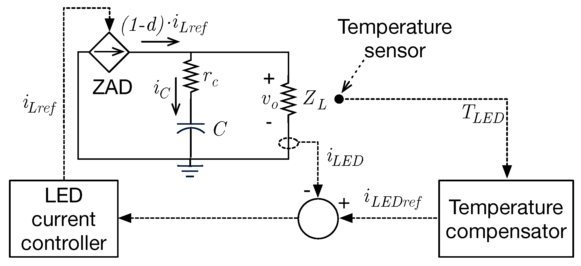
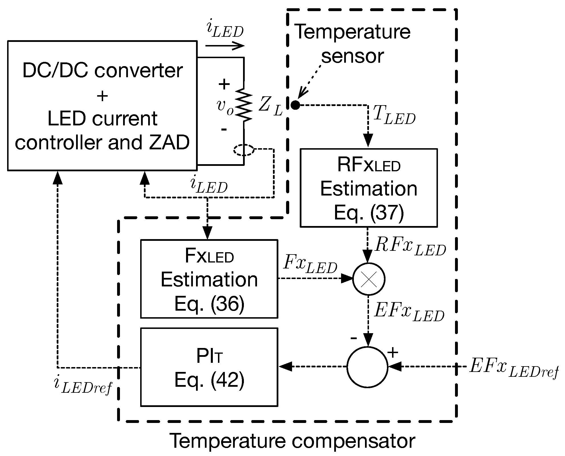
2.1. General Diagram

Figure 1 shows the general diagram of the system considered in the research. The circuit includes a buck-boost converter where parasitic resistances and voltage drops in the diode are included in the model. The lower right side of the diagram shows a PID control that uses the current signal through the LEDS ($i_{LED}$) and an output signal from the temperature compensator ($i_{LEDref}$) to obtain the reference current ($i_{Lref}$) that is passed to the inductor current control. The lower left of the diagram shows a ZAD controller that uses the reference current ($i_{Lref}$) and the inductor current measured in the systems ($i_L$) to calculate the error (e) and obtain the duty cycle that generates a PWM signal that controls the MOSFET.

The performance of the proposed solution is tested by considering a portable LED light consisting of three groups of LEDs connected in series. The solution is designed to obtain a current through the LEDs that maintains a similar luminous flux.

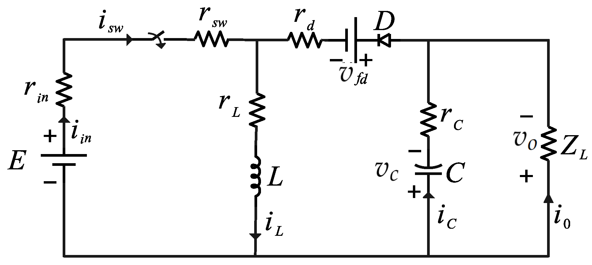
2.2. Electrical Circuit Model

The electrical model of the power system, based on a buck-boost converter, is depicted in Figure 2. All parasitic losses are considered to ensure an accurate description of the system behavior. This circuit models the battery ($E=v_{in}\left(t\right)$) and its internal resistance ($r_{in}$), and also considers the conduction resistance ($r_{sw}$) of the MOSFET channel N. In addition, the inductance (L) includes the parasitic resistance ($r_L$) and the capacitance (C) includes the corresponding parasitic resistance ($r_C$). Furthermore, the diode (D) considers both the resistance ($r_d$) and the forward voltage ($v_{fd}$). Finally, the load is connected to the circuit and represented as ($Z_L$).

The mathematical model of this circuit is obtained as follows. The differential equations of both the inductor current and capacitor voltage are obtained for both states of the switch, and then those equations are combined in the switched model.

The first condition of the circuit occurs when the switch is closed (ON), which forces the diode to be open, enabling the input source (E = $v_{in}\left(t\right)$) to feed the circuit. In this case, the input current is equal to the inductor current ($i_{in}=i_L$), while the capacitor supplies the load power. The differential equations in this state are expressed as in Equations (1) and (2).

$$\dot{x_1}={\displaystyle \frac{d{v}_c\left(t\right)}{dt}}={\displaystyle \frac{-1}{C(r_c+Z_L)}}{v}_c\left(t\right)$$

(1)

$$\dot{x_2}={\displaystyle \frac{d{i}_L\left(t\right)}{dt}}={\displaystyle \frac{-\left[r_{in}+r_{sw}+r_L\right]}{L}}{i}_L\left(t\right)+{\displaystyle \frac{v_{in}\left(t\right)}{L}}$$

(2)

In a compact form, it can be written as in Equations (3) and (4).

$$\dot{x_1}=b{x}_1\left(t\right)$$

(3)

and

$$\dot{x_2}=a{x}_2\left(t\right)+{\displaystyle \frac{v_{in}\left(t\right)}{L}}$$

(4)

where a and b are parameters given in Equations (5) and (6).

$$a=-\left[{\displaystyle \frac{r_{in}+r_{sw}+r_L}{L}}\right],$$

(5)

$$b={\displaystyle \frac{-1}{C(r_c+Z_L)}}.$$

(6)

Finally, the load voltage ($v_o\left(t\right)$) is calculated as in Equation (7)

$$v_o\left(t\right)=\left(1-{\displaystyle \frac{r_c}{r_c+Z_L}}\right)v_c\left(t\right)$$

(7)

The second condition occurs when the switch is open (OFF), which forces the diode to close, isolating the input source from the circuit. In this case, the input current is equal to zero ($i_{in}=0$), while the inductor feeds both the capacitor and the load. The differential equations in this second state are presented in Equations (8) and (9).

$$\dot{x_1}={\displaystyle \frac{d{v}_c\left(t\right)}{dt}}={\displaystyle \frac{Z_L}{C(Z_L+r_c)}}{i}_L\left(t\right)-{\displaystyle \frac{1}{C(Z_L+r_c)}}{v}_c\left(t\right)$$

(8)

$$\dot{x_2}={\displaystyle \frac{d{i}_L\left(t\right)}{dt}}=-\left(r_L+r_d+{\displaystyle \frac{Z_L{r}_c}{Z_L+r_c}}\right){\displaystyle \frac{i_L\left(t\right)}{L}}-\left({\displaystyle \frac{Z_L}{Z_L+r_c}}\right){\displaystyle \frac{v_c\left(t\right)}{L}}-{\displaystyle \frac{v_{fd}}{L}}$$

(9)

In a compact form, it can be written as in Equations (10) and (11).

$$\dot{x_1}=g{x}_2\left(t\right)+f{x}_1\left(t\right)$$

(10)

$$\dot{x_2}=p{x}_2\left(t\right)+m{x}_1\left(t\right)-{\displaystyle \frac{v_{fd}}{L}}$$

(11)

where g, f, p, and m are parameters given in Equations (12) and (13).

$$g={\displaystyle \frac{Z_L}{C(Z_L+r_c)}},f=-{\displaystyle \frac{1}{C(Z_L+r_c)}}$$

(12)

$$p=-{\displaystyle \frac{1}{L}}\left(r_L+r_d+{\displaystyle \frac{Z_L{r}_c}{Z_L+r_c}}\right),m=-{\displaystyle \frac{1}{L}}\left({\displaystyle \frac{Z_L}{Z_L+r_c}}\right).$$

(13)

Finally, the load voltage ($v_o\left(t\right)$) is calculated with Equation (14).

$$v_o\left(t\right)={\displaystyle \frac{r_c{Z}_L}{Z_L+r_c}}{i}_L\left(t\right)+\left(1-{\displaystyle \frac{r_c}{Z_L+r_c}}\right)v_c\left(t\right)$$

(14)

Combining the previous differential equations, using the control signal of the switch (u), where $u=1$ closes the switch and $u=0$ opens the switch ($\overline{u}=1-u$), leads to the following switched model (Equations (15) and (16)):

$$\begin{array}{c}\hfill {\displaystyle \frac{d{i}_L\left(t\right)}{dt}}=-\left[\left(r_{sw}+r_{in}\right)u+\left(r_d+{\displaystyle \frac{Z_L{r}_c}{Z_L+r_c}}\right)\overline{u}+r_L\right]{\displaystyle \frac{i_L\left(t\right)}{L}}-...\\ \hfill \left({\displaystyle \frac{Z_L}{Z_L+r_c}}\right)\overline{u}{\displaystyle \frac{v_c\left(t\right)}{L}}-{\displaystyle \frac{v_{fd}}{L}}\overline{u}+{\displaystyle \frac{v_{in}}{L}}u\end{array}$$

(15)

$${\displaystyle \frac{d{v}_c\left(t\right)}{dt}}={\displaystyle \frac{Z_L}{C(Z_L+r_c)}}{i}_L\left(t\right)\overline{u}-{\displaystyle \frac{1}{C(Z_L+r_c)}}{v}_c\left(t\right)$$

(16)

where the load voltage ($v_o\left(t\right)$) is calculated with Equation (17) and the battery current ($i_{in}\left(t\right)$) is calculated with Equation (18).

$$v_o\left(t\right)={\displaystyle \frac{r_c{Z}_L}{Z_L+r_c}}\overline{u}{i}_L\left(t\right)+\left(1-{\displaystyle \frac{r_c}{Z_L+r_c}}\right)v_c\left(t\right)$$

(17)

$$i_{in}\left(t\right)=u{i}_L\left(t\right)$$

(18)

The previous model describes both the average value and switching ripple of all the currents and voltages, which is needed for the controller designed in this paper. However, for the design of the passive elements and testing purposes, the averaged model is often used, which disregards the switching ripple. Considering that the average value of the control signal u is equal to the duty cycle, i.e., $d={\displaystyle \frac{1}{T}}{\int }_0^{T}udt$ where T is the duration of the switching period of the pulse-width modulator (PWM) and $d\prime =1-d$, the averaged value is calculated as follows:

$$\begin{array}{c}\hfill {\displaystyle \frac{d{i}_L\left(t\right)}{dt}}=-\left[\left(r_{sw}+r_{in}\right)d+\left(r_d+{\displaystyle \frac{Z_L{r}_c}{Z_L+r_c}}\right)d^{\prime }+r_L\right]{\displaystyle \frac{i_L\left(t\right)}{L}}-...\\ \hfill \left({\displaystyle \frac{Z_L}{Z_L+r_c}}\right)d^{\prime }{\displaystyle \frac{v_c\left(t\right)}{L}}-{\displaystyle \frac{v_{fd}}{L}}{d}^{\prime }+{\displaystyle \frac{v_{in}}{L}}d\end{array}$$

(19)

$${\displaystyle \frac{d{v}_c\left(t\right)}{dt}}={\displaystyle \frac{Z_L}{C(Z_L+r_c)}}{i}_L\left(t\right)d\prime -{\displaystyle \frac{1}{C(Z_L+r_c)}}{v}_c\left(t\right)$$

(20)

$$v_o\left(t\right)={\displaystyle \frac{r_c{Z}_L}{Z_L+r_c}}d\prime i_L\left(t\right)+\left(1-{\displaystyle \frac{r_c}{Z_L+r_c}}\right)v_c\left(t\right)$$

(21)

$$i_{in}\left(t\right)=d{i}_L\left(t\right)$$

(22)

2.3. ZAD Control

The switching surface in this research is chosen as expressed in Equation (23)

$$S\left(\mathbf{x}\left(t\right)\right)=(x_2\left(t\right)-x_{2\mathrm{ref}}\left(t\right))+k_1\left[{\dot{x}}_2\left(t\right)-{\dot{x}}_{2ref}\left(t\right)\right].$$

(23)

where, $k_1=-10\sqrt{LC}$.

The numerical simulations are performed employing the pulse width modulation (PWM) scheme. Hence, the duty cycle is given by the expression in Equation (24).

$$d_{ZAD}={\displaystyle \frac{2S\left(\mathbf{x}\left(t\right)\right)+T{S}^{-}\left(\mathbf{x}\left(t\right)\right)}{S^{-}\left(\mathbf{x}\left(t\right)\right)-S^{+}\left(\mathbf{x}\left(t\right)\right)}},$$

(24)

where $S^{-}$ and $S^{+}$ correspond to the derivatives of the switching surface when $u=1$ and $u=0$, as expressed in Equation (25).

$$S^{+}\left(\mathbf{x}\left(t\right)\right)=\dot{S}\left(\mathbf{x}\left(t\right)\right){|}_{u=1}\mathrm{and}{S}^{-}\left(\mathbf{x}\left(t\right)\right)=\dot{S}\left(\mathbf{x}\left(t\right)\right){|}_{u=0}.$$

(25)

In this case, $S^{+}$ and $S^{-}$ are given by Equation (26).

$$\begin{array}{cc}\hfill S^{+}\left(\mathbf{x}\left(t\right)\right)& =(1+a{k}_1)\left[a{x}_2\left(t\right)+{\displaystyle \frac{v_{in}\left(t\right)}{L}}\right],\hfill \\ \hfill S^{-}\left(\mathbf{x}\left(t\right)\right)& =(1+p{k}_1)\left[p{x}_2\left(t\right)+m{x}_1\left(t\right)-{\displaystyle \frac{v_{fd}}{L}}\right]+m{k}_1\left[g{x}_2\left(t\right)+f{x}_1\left(t\right)\right].\hfill \end{array}$$

(26)

2.4. LED Current Control

The correct operation of the ZAD controller makes possible to model the diode as a current source with a gain equal to $1-d$. Based on this consideration, the equivalent circuit of the output node is reported in Figure 3. This figure also includes a cascade LED current controller, which automatically defines the reference value of the ZAD controller. Moreover, the figure considers the temperature compensator, which defines the LED current reference, thus ensuring a regulated luminous flux produced by each group of LED.

The differential equation in the capacitor is given in Equation (27). The Laplace domain leads to the transfer function given in Equation (28) between the current of the LED $i_{LED}$ and the current of the inductor regulated by the ZAD controller $i_{Lref}$.

$$\begin{array}{c}\hfill i_c=i_L\left(1-d\right)-{\displaystyle \frac{v_c+i_c{r}_c}{Z_L}}\to C\left(Z_L+r_c\right){\displaystyle \frac{d{v}_c}{dt}}+v_c=i_L\left(1-d\right)Z_L\end{array}$$

(27)

$$\begin{array}{cc}\hspace{1em}\hspace{1em}\hspace{1em}\hspace{1em}\hspace{1em}\hspace{1em}\hspace{1em}\hspace{1em}& \hfill {\displaystyle \frac{i_{LED}}{i_{Lref}}}=G_{LED}={\displaystyle \frac{\left(1+sC{r}_c\right)\left(1-d\right)}{C\left(Z_L+r_c\right)s+1}}\end{array}$$

(28)

Considering that the ESR resistance ($r_c$) of the output capacitor is small with respect to both the impedance $Z_L$ of commercial LEDs and the impedance of the capacitor at the natural frequency, the previous transfer function can be simplified as in Equation (29).

$$\begin{array}{c}\hfill G_{LED}\approx {\displaystyle \frac{1-d}{C{Z}_{L}s+1}}\mathsf{if}\left\{{\displaystyle \frac{r_c}{Z_L}}<<1\mathsf{and}{r}_c{\omega }_{n}C<<1\right\}\end{array}$$

(29)

The LED current controller is designed with a PI structure as presented in Equation (30), which leads to the closed-loop transfer function between the LED current ($i_{LED}$) and the desired value ($i_{LEDref}$) given in Equation (31).

$$\begin{array}{cc}\hspace{1em}\hspace{1em}\hspace{1em}\hspace{1em}\hspace{1em}& \hfill G_{cv}=k_p+{\displaystyle \frac{k_i}{s}}\end{array}$$

(30)

$$\begin{array}{c}\hfill {\displaystyle \frac{i_{LED}}{i_{LEDref}}}={\displaystyle \frac{\frac{1-d}{Z_{L}C}\left(s{k}_p+k_i\right)}{s^2+\frac{1+k_p\left(1-d\right)}{Z_{L}C}s+\frac{k_i\left(1-d\right)}{Z_{L}C}}}\end{array}$$

(31)

Contrasting the denominator of (31) with the canonical second-order transfer function $s^2+2\rho {\omega }_{n}s+{\omega }_n^2$, and taking into account that the settling time (in the 2% band) of a second-order system is approximated by $t_s={\displaystyle \frac{3.9}{\rho {\omega }_n}}$, then the natural frequency ${\omega }_n$ of the closed-loop system is calculated as given in Equation (32). Finally, the parameter $k_p$ is calculated in Equation (33) to impose the desired settling time $t_s$, while the parameter $k_i$ is calculated in Equation (34) to impose the desired damping ratio for the LED current.

$$\begin{array}{cc}\hspace{1em}\hspace{1em}\hspace{1em}\hspace{1em}& \hfill {\omega }_n={\displaystyle \frac{3.9}{\rho t_s}}\end{array}$$

(32)

$$\begin{array}{c}\hfill k_p={\displaystyle \frac{1}{1-d}}\left[{\displaystyle \frac{7.8Z_{L}C}{t_s}}-1\right]\end{array}$$

(33)

$$\begin{array}{cc}\hspace{1em}\hspace{1em}& \hfill k_i={\displaystyle \frac{Z_{L}C}{1-d}}{\left({\displaystyle \frac{3.9}{\rho t_s}}\right)}^2\end{array}$$

(34)

This control structure and parameters design will be tested in the next section.

2.5. Parameters of the Circuit

The solution considers groups of LEDs producing 2000 lm, which is equivalent to 150 W bulb lamps, hence the complete light system can produce 6000 lm (3 groups), 4000 lm (2 groups) or 2000 lm (1 group) depending on the user requirement or battery charge. The particular LED adopted is the MP-5050-240E [19], which produces a maximum of 1000 lm at 850 mA and 6.4 V. In order to avoid the LED operation at the maximum rating, and to provide an additional operation range to compensate for temperature effects, each LED is operated at 667 lm. Thus, each group of LEDs is formed by three MP-5050-240E connected in parallel.

The parameters used in the system analysis are those described in

Table 1. Parameter used in the simulation of the circuit with the buck-boost converter.

Parameters	Value
Input Voltage $E=$ $v_{\mathrm{in}}\left(t\right)$	12 VDC
Source Resistance $r_{\mathrm{in}}$	0.3 $\Omega$
Inductor L	0.784 mH
Inductor Resistance $r_L$	0.2 $\Omega$
Diode Forward Voltage $V_{f_d}$	0.7 V
Diode Resistance $r_d$	0.03 $\Omega$
MOSFET Switch Resistance $r_{\mathrm{sw}}$	0.0175 $\Omega$
Capacitance C	132 $\mathsf{\mu }\mathrm{F}$
Capacitor Resistance $r_c$	0.05 $\Omega$
Impedance per group $Z_L$	3.9375 $\Omega$
Control parameter with ZAD $k_1$	−0.0032
Switching Frequency $f_{\mathrm{sw}}$ = $F_s$	20 kHz
PI Controller Proportional Gain $k_p$	3.4905 A/A
PI Controller Integral Gain $k_i$	5627.1 A/s
Thermal Resistance (steady state) $R_{\mathrm{th}}$	2 °C/W
Ambient Temperature $T_a$	30 °C

. The battery has an open circuit voltage $v_{\mathrm{in}}\left(t\right)=12\mathrm{VDC}$ and an internal resistance $r_{\mathrm{in}}=0.3\Omega$. The inductance of the converter is $L=0.784\mathrm{mH}$, with an internal resistance of $r_L=0.2\Omega$. The diode used has a forward voltage of $v_{fd}=0.7\mathrm{V}$ and an internal resistance of $r_d=0.03\Omega$. The internal resistance of the MOSFET switch is $r_{\mathrm{sw}}=0.0175\Omega$. The output capacitance C is formed by fours capacitors of $33\mathsf{\mu }\mathrm{F}$ and an internal resistance of $0.2\Omega$ each one of them, hence $C=132\mathsf{\mu }\mathrm{F}$ and $r_c=0.05\Omega$. Since the MP-5050-240E LED has a 1000 lm operation point with 800 mA and 6.3 V, the impedance of each group of LEDs is $Z_L=3.9375\Omega$ with 1.6 A and 6.3 V, the impedance of two groups is $Z_L=7.8740\Omega$ (1.6 A and 12.6 V), and the impedance of three groups is $Z_L=11.8125\Omega$ (1.6 A and 18.9 V). The control parameter with ZAD, $k_1$, is set to $-0.0032$ for all tests. Finally, the switching frequency of the MOSFET is $f_{\mathrm{sw}}=20\mathrm{kHz}$.

2.6. Parameters of the LED Current Controller and Batteries

The energy requirement of the light system is mainly imposed by the current of the LED and the desired service time. Considering that the current of the groups of LEDs is regulated at 1.6 A to ensure a uniform 2000 lm illumination per group, each group of LEDs will consume 1.6 Ah to provide the same luminous flux for one hour.

Table 2. Example of battery service times per group.

Battery	Voltage (V)	Capacity (Ah)	Cost (USD)	Service Time (h)
CA1233	12	3.3	$11.56	2
BW 1280 F1	12	8	$24.99	5
PC36-12NB	10.5	38.6	$81.75	24

reports examples of the service time provided by some commercial batteries for a single group of LEDs. For example, the CA1233 battery will ensure 2000 lm for two hours (one active group of LEDs), 4000 lm for one hour (2 active groups of LEDs), or 6000 lm for 40 min (3 active groups of LEDs). Similarly, the PC36-12NB battery will supply 2000 lm for 24 h (1 active group of LEDs), 4000 lm for 12 h (2 active group of LEDs) or 6000 lm for 8 h (3 active groups of LEDs). Therefore, the number of active groups of LEDs can be adjusted depending on the light (luminous flux) and service time required. It should be noted that the PC36-12NB battery has a nominal voltage equal to 10.5 V, which can be used since the proposed power circuit is based on a step-up/down converter (buck-boost), thus providing flexibility in the selection of the battery voltage. Finally, it is observed that the largest battery (PC36-12NB) provides 12 times the service time of the smaller battery (CA1233) with 7 times the cost, while the medium battery (BW 1280 F1) provides 2.5 times the service time of CA1233 with 2.2 times the cost. Therefore, increasing the battery capacity produces a proportional increase in service time with a smaller proportion of the cost increase.

Concerning the parameters of the LED current controller, it is designed to achieve a settling time $t_s$ lower than 3 ms and a damping ratio $\rho =0.8$, which provides a balance between the response time and the maximum overshoot. The first step is to verify the conditions $r_c$ specified in Equation (29) for the simplification of the transfer function $G_{LED}$: ${\displaystyle \frac{rc}{Z_L}}=0.0127<<1$ and $r_c{\omega }_{n}C=0.0107<<1$, where ${\omega }_n=1.6250$ krad/s is calculated from (32). Figure 4a shows the comparison between the exact output node model presented in Equation (28) and the approximation reported in Equation (29), where the correct behavior of the approximated model is evident, hence the control design equations are precise.

Finally, $k_p=3.4905A/A$ is calculated from (33) and $k_i=5.6271kA/\mathsf{s}$ is calculated from (34). The normalized closed-loop response of the output node, under the action of the designed LED current controller (30), is tested using exact and approximate models. Figure 4b shows this simulation results, which confirms the correct operation of the controller with both models; in fact, both models achieve the same desired settling time with the same overshoot. Therefore, it can be used with the real power circuit.

2.7. Temperature Compensation and Luminous Flux Regulation

The luminous flux produced by the LED MP-5050-240E is affected by the operating temperature. Thus, a current compensation is required to ensure a constant luminous flux during the LED operation. The design of this temperature-based current compensation requires to model four relations inside the LED:

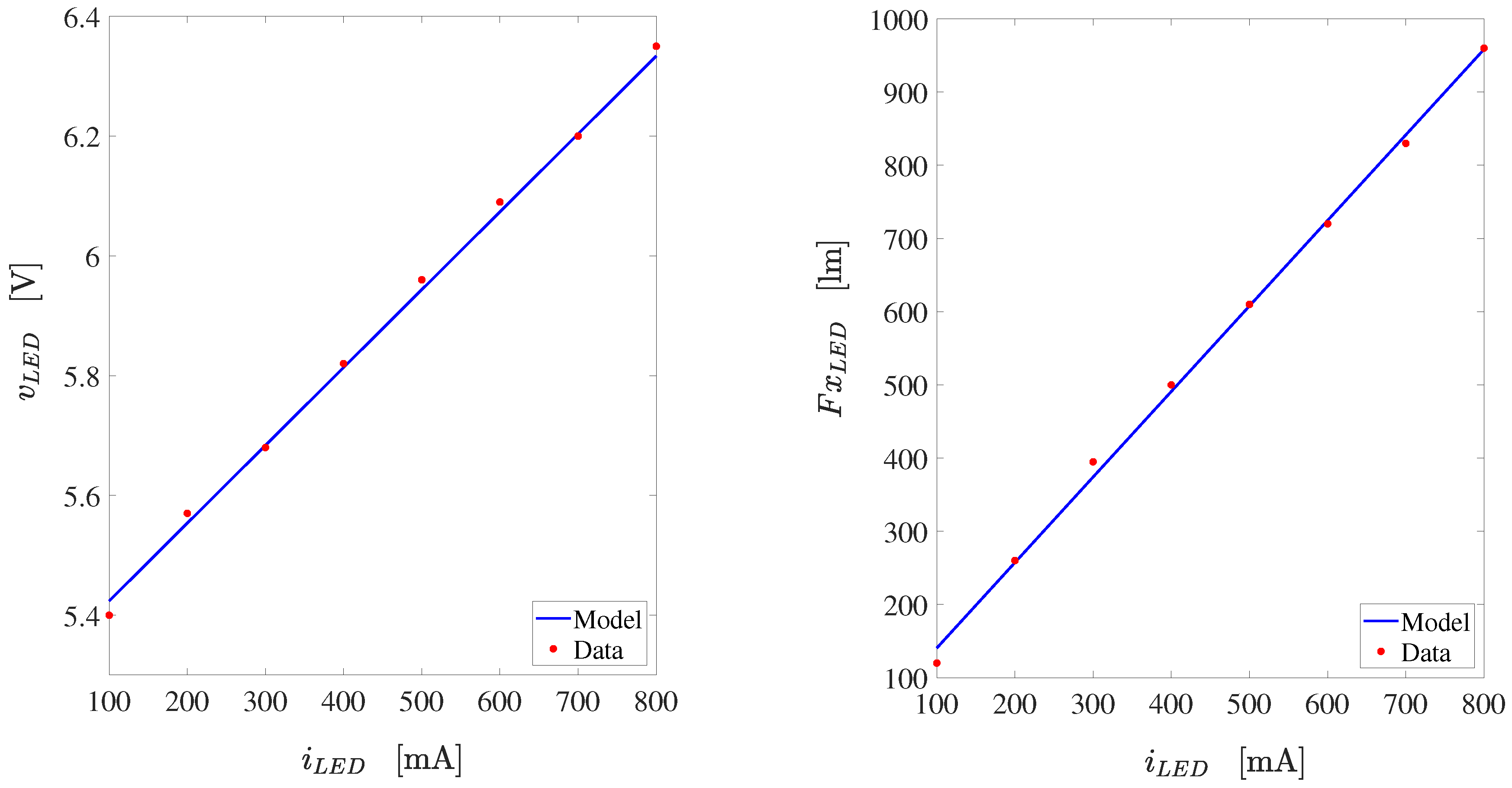
• The voltage vs. current relation.
• The luminous flux vs. current relation.
• The luminous flux vs. temperature relation.
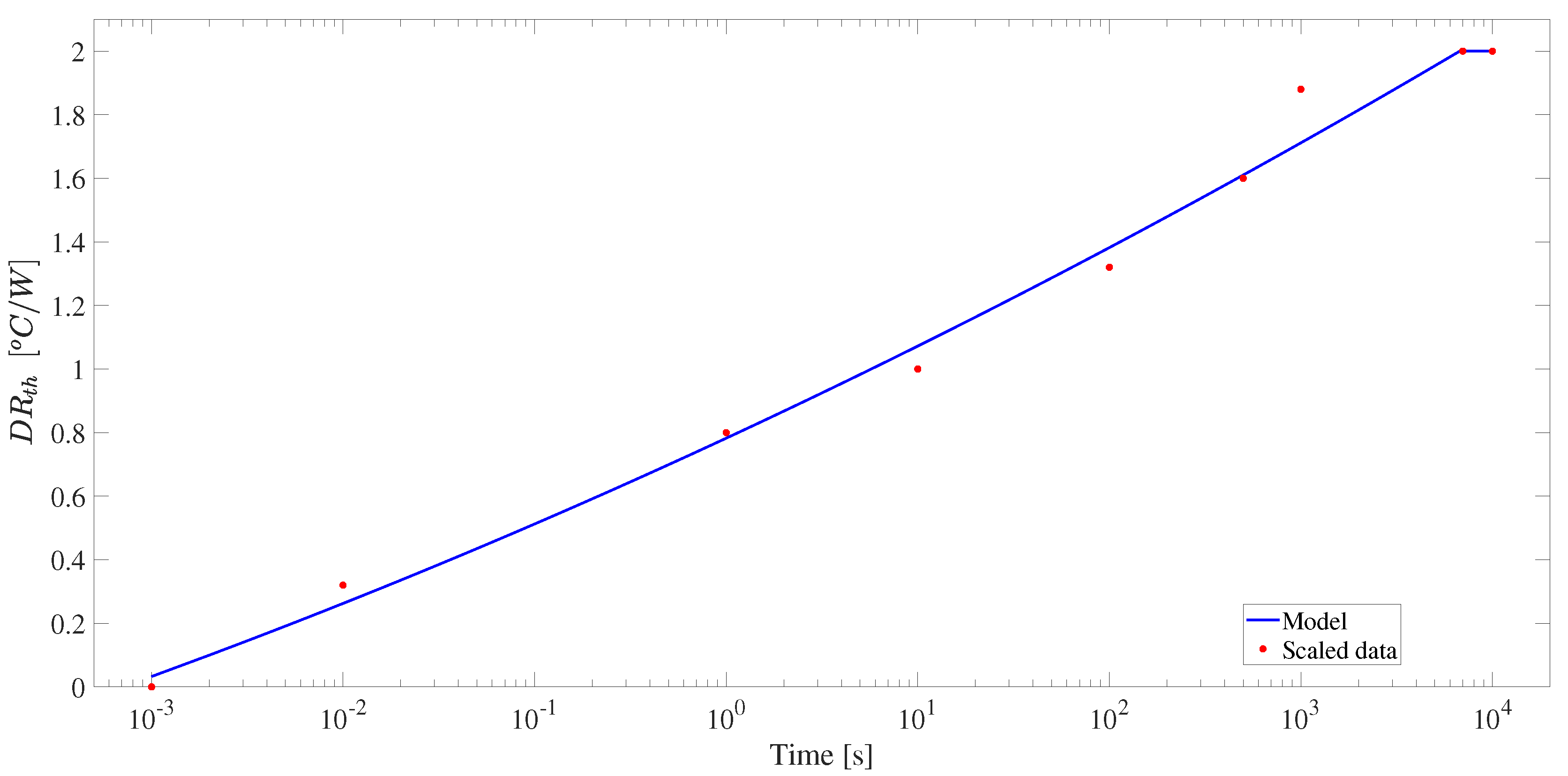
• The temperature variation vs. the operating time.

The datasheet of the LED MP-5050-240E [19] provides data for the first three relations. The voltage vs. current relation is modeled using the expression given in (35), where increments in the LED current $i_{LED}$ (mA) also produce increments in the LED voltage $v_{LED}$ (V). The luminous flux vs. current relation is modeled using expression (36), where increments in the LED current (mA) also increase the luminous flux $F{x}_{LED}$ (lm) produced by the LED. Figure 5 shows the data extracted from the manufacturer’s datasheet and the modeling expressions reported in (35) and (36), where a satisfactory agreement is achieved.

$$\begin{array}{cc} & \hfill v_{LED}=0.0013·i_{LED}+5.2936\end{array}$$

(35)

$$\begin{array}{c}\hfill F{x}_{LED}=1.1685·i_{LED}+23.5714\end{array}$$

(36)

The data provided by the manufacturer’s datasheet about the reduction in luminous flux caused by the temperature of the LED is normalized. Hence, it is given as a relative luminous flux ($RF{X}_{LED}$) vs. temperature ($T_{LED}$) relation. Equation (37) provides a polynomial expression that models such a relative luminous flux (%) for different temperatures (°C). Finally, the effective luminous flux ($EF{x}_{LED}$) produced by the LED, for different temperatures, is calculated by multiplying the theoretical luminous flux (36) by the relative luminous flux (37), thus resulting in Equation (38).

$$\begin{array}{c}\hfill RF{x}_{LED}=-5.5592\times {10}^{-6}·T_{LED}^2-5.0571\times {10}^{-4}·T_{LED}+1.0154\end{array}$$

(37)

$$\begin{array}{cc}\hspace{1em}\hspace{1em}\hspace{1em}\hspace{1em}\hspace{1em}\hspace{1em}\hspace{1em}\hspace{1em}\hspace{1em}& \hfill EF{x}_{LED}=F{x}_{LED}·RF{x}_{LED}\end{array}$$

(38)

Figure 6 shows the $RF{x}_{LED}$ data extracted from the Manufacturer’ datasheet, moreover the satisfactory agreement of the modeling expression (37) is observed. Then, Equation (38) is used to calculate the effective luminous flux $EF{x}_{LED}$ produced by the LED for different current and temperature conditions.

The temperature variation vs. operation time relation is not reported in the manufacturer’s datasheet. However, the work published in [20] reports experimental measurements of changes in thermal resistance during the stabilization time of the LED, for three different commercial LEDs. That work shows the same dynamic behavior for the three LEDs, and the main difference corresponds to the steady-state (final) value, which is equal to the thermal resistance $R_{th}$ reported in the manufacturer’s datasheet. Those experimental data were normalized with the $R_{th}$ value of each LED to produce a relative thermal resistance behavior $R{R}_{th}$ (%), which is modeled by expression (39). This expression is a polynomial calculation based on the logarithm of the operation time, and the maximum value of $R{R}_{th}$ is $100\%$. Finally, the dynamic behavior of the thermal resistance $D{R}_{th}$ in the LED MP-5050-240E is obtained by multiplying $R{R}_{th}/100$ by the static thermal resistance $R_{th}=2$ °C/W reported in [19], as given in (40). Figure 7 shows the scaled data and dynamic model behavior of the thermal resistance MP-5050-240E, where the expression (40) provides a satisfactory performance. It is observed that the thermal stabilization of the LED occurs around 70,000 s, i.e., 1 h and 57 min. In addition, the change in the temperature of the LED is calculated by multiplying the dynamic thermal resistance and the power of the LED.

$$\begin{array}{c}\hfill R{R}_{th}=0.4980·log{\left(t\right)}^2+13.9903·log\left(t\right)+39.1209\wedge max\left(R{R}_{th}\right)=100\end{array}$$

(39)

$$\begin{array}{cc}\hspace{1em}\hspace{1em}\hspace{1em}\hspace{1em}\hspace{1em}\hspace{1em}\hspace{1em}\hspace{1em}\hspace{1em}\hspace{1em}\hspace{1em}\hspace{1em}\hspace{1em}\hspace{1em}& \hfill D{R}_{th}={\displaystyle \frac{R_{th}·R{R}_{th}}{100}}\end{array}$$

(40)

Figure 7 shows that the dynamic thermal resistance of the LED increases over the operation time, which reduces the effective luminous flux $EF{x}_{LED}$ as observed in Figure 6. The simulation of the dynamic behavior of the LED is performed as follows:

• Set the LED current $i_{LED}$ to the desired value.
• Calculate the LED voltage $v_{LED}$ using (35) and the LED power as $P_{LED}=i_{LED}·v_{LED}$.
• The dynamic thermal resistance $D{R}_{th}$ is calculated from (39) and (40) for the particular time instant of the simulation.
• The increment in the LED temperature is calculated as $\Delta T_{LED}=D{R}_{th}·P_{LED}$. Then, the LED temperature is calculated by adding the ambient temperature $T_a$ as $T_{LED}=\Delta T_{LED}+T_a$.
• The theoretical luminous flux $F{x}_{LED}$ of the LED is calculated from (36).
• The relative luminous flux $RF{x}_{LED}$ caused by the LED temperature is calculated from (37).
• Finally, the effective luminous flux $EF{x}_{LED}$ produced by the LED, due to the temperature effect, is calculated from (38).

Figure 6 put into evidence that keeping constant the effective luminous flux produced by the LED requires to increase the LED current over the operation time. Therefore, each LED must be start operating below its maximum rating; for the LED MP-5050-240E it is 800 mA. To achieve the desired 2000 lm in each LED group requires providing $666.67$ lm in each parallel-connected LED (3 LEDs form a group), and the current in each LED group is calculated multiplying by 3 expression (36). Moreover, since the LEDs in each group are close, the temperature increase is equal to multiplying by 3 the $\Delta T_{LED}$ produced by a single LED.

In order to produce the desired 2000 lm it required a theoretical group LED current equal to 1.65 A, which is calculated from (36). Setting such a current, and executing the previous simulation steps, produce the dynamic simulation of a LED group reported in Figure 8. This figure shows the dynamic thermal resistance, without a logarithmic axis, that reaches the expected steady-state value, that is, the manufacturer $R_{th}$. The LED group temperature $T_{LED}$ starts at the ambient temperature, which in this simulation is considered $T_a=30$ °C, reaching a steady-state value equal to 50 °C. This temperature increase reduces the relative luminous flux $RF{x}_{LED}$ of the LED group, also reducing the effective luminous flux $EF{x}_{LED}$ produced by the LED group.

The previous simulation confirms that the current of the LED group must be adjusted to compensate for the temperature effect on the effective luminous flux $EF{x}_{LED}$ produced by the LED group. From simulation data between 0 and 1 s, the dynamic relation between $EF{x}_{LED}$ and $i_{LED}$ is calculated as the following transfer function:

$$\begin{array}{c}\hfill G_{EFx}\left(s\right)={\displaystyle \frac{EF{X}_{LED}\left(s\right)}{i_{LED}\left(s\right)}}={\displaystyle \frac{13.44}{0.25s+1}}\end{array}$$

(41)

Using the root-locus technique, the temperature-compensation PI controller given in (42) is calculated to ensure a settling time of 0.5 s. The processing of this controller requires measuring the temperature of the LED group, which is used to estimate the effective luminous flux $EF{x}_{LED}$: $i_{LED}$ is known (already measured for the current control), $F{X}_{LED}$ is calculated from (36), $EF{x}_{LED}$ is estimated from (37) and (38), and such an estimation is compared with the desired luminous flux $EF{x}_{LEDref}$ to calculate the error. Finally, that error is processed with the $P{I}_T$ controller to generate the reference $i_{LEDref}$ for the LED current controller. Figure 9 shows the block diagram of this temperature compensator, which only requires an additional temperature sensor for the LED group and the information provided in the manufacturer’s datasheet.

$$\begin{array}{c}\hfill P{I}_T\left(s\right)={\displaystyle \frac{0.6·s+12}{s}}\end{array}$$

(42)

In conclusion, this temperature compensator ensures the production of the desired luminous flux in each LED group.

3. Results and Analysis

This section presents results from the simulation of the luminous flux regulation to different values, accounting for the temperature effect, and considering different commercial batteries.

3.1. Tests Performed in the System

The evaluation of the proposed solution is performed with detailed circuit simulations executed in Matlab Simulink 2018a. Due to the wide difference between the time responses of the LED current and LED temperature, three kind of simulations were conducted: verification of the ZAD and LED current controllers tracking the LED current reference for different batteries, which requires short simulations of 0.06 s; verification of the ZAD and LED current controllers to battery discharge, which requires simulations of 6 s; verification of the luminous flux regulation at the LED start-up, which requires simulations of 1 s; and verification of the luminous flux regulation for long time frames to account for the temperature effect, which requires to simulate 1 h and 57 min of operation. All simulations were implemented using a fixed-step size solver, where the fundamental sample time is defined as $1/(\Delta ·F_s)$, with $\Delta =1000$ and $F_s=20000$ Hz, corresponding to the PWM switching frequency. The solver used was Ode1 (Euler) with solver selection type: fixed-step and periodic sample time constraint: unconstrained.

To ensure realistic simulation results, all battery-related parameters used in the tests were based on real commercial models. The values for voltage, capacity, and cost were extracted from datasheets and market sources. These parameters were used to configure the Simulink battery blocks appropriately, enabling accurate modeling of discharge behavior and energy availability. In summary, the tests are presented below, and the actual batteries used, along with their specifications, are listed in

Table 3. Overview of commercial batteries used in the system.

Battery	Battery Chemistry	Voltage (V)	Capacity (Ah)	Cost (USD)	Service Time at 5 A
BW 1280 F1	Lead Acid	12	8	$24.99	1.6 h
TOOL-486LI-30	Lithium Ion	18	3	$38.69	0.6 h
UPS-BAT/VRLA-WTR	Lead Acid	24	13	$695.54	2.4 h
CUSTOM-334	Nickel Metal Hydride	12	0.4	$25.58	288 s

.

• Test 1: LED current control in boost mode with a 12-volt battery.
• Test 2: LED current control in buck-boost mode with a 18-volt battery.
• Test 3: LED current control in buck mode with a 24-volt battery.
• Test 4: LED current control with a discharged 12-volt battery.
• Test 5: luminous flux regulation, testing the LED start-up and long time operation.

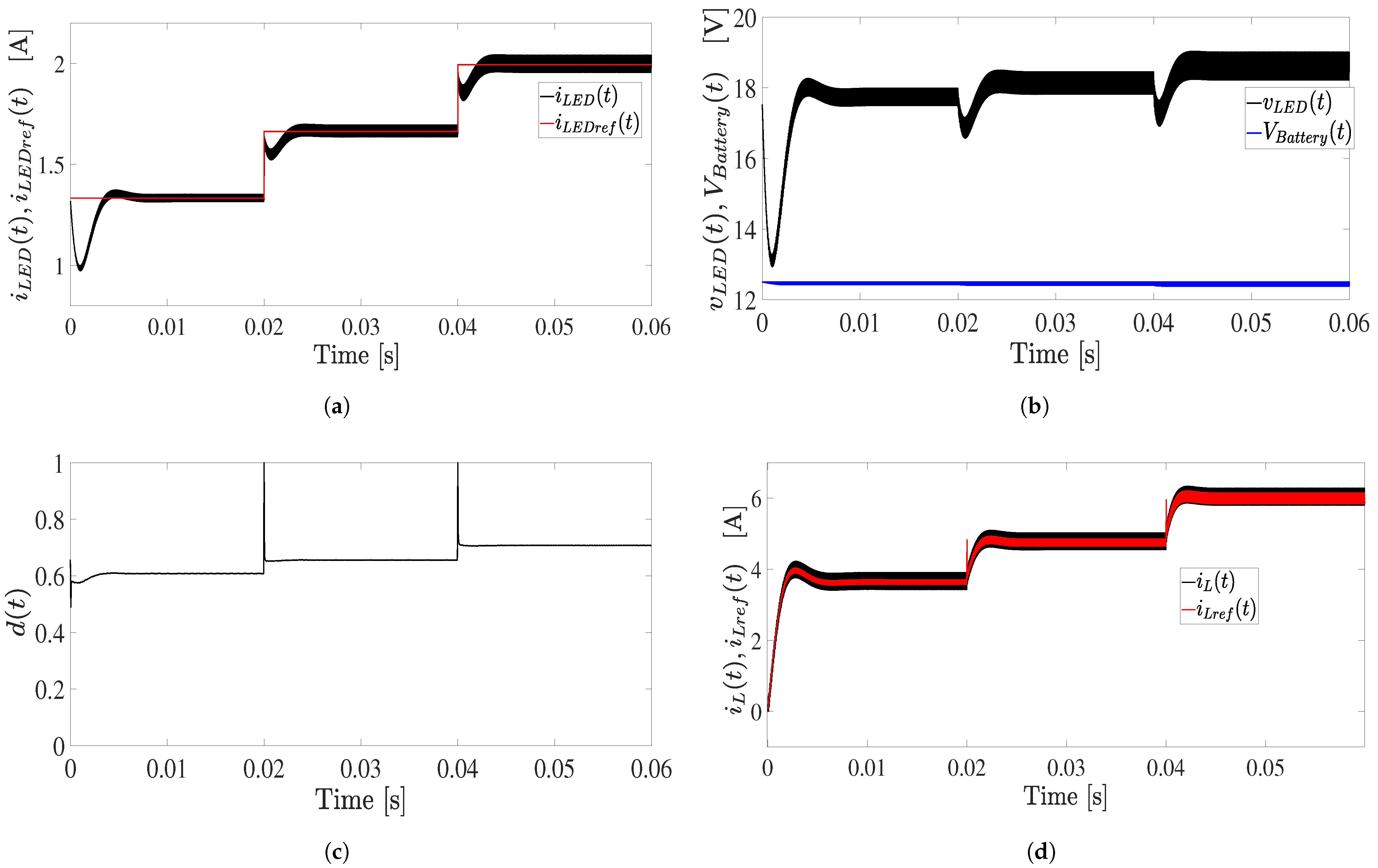
3.2. Test 1: LED Current Control in Boost Mode

Figure 10 presents the behavior of the system when you have a real 12-volt lead acid battery (BW 1280 F1), which puts the system in boost mode according to the voltage of the LEDs.

Figure 10a shows the current in the LEDs ($i_{LED}$) and the reference current ($i_{Lref}$). This figure shows that an event was performed in which $i_{LEDref}$ is started at 1.3324 A (red color) for 0 to 20 ms, which corresponds to a luminous flux of 4900 lm generated by the set of LEDs, requiring a voltage in the LEDs of 17.61 V. Then, the $i_{LEDref}$ is changed to 1.663 A and maintained for 20 ms to 40 ms, generating 6000 lm for the LED array, and requiring a total voltage of 18 V. Finally, $i_{LEDref}$ is changed to 1.9936 A, and maintained from 40 ms to 60 ms, generating 7200 lm for the LEDs, and requiring a total voltage of 18.48 V. The simulation shows that the $i_{LED}$ signal correctly follows the reference signal $i_{LEDref}$, showing that the ZAD control objective and the LED current control objective is met. It is also observed that there are no overimpulses, and the response is met with the defined settling time (3 ms). As the reference signal ($i_{LEDref}$) increases, the controlled signal ($i_{LED}$) has a greater amplitude in the ripple; however, this ripple has a maximum value of 4.22%.

Figure 10b shows the voltage in the LEDs (black) and the voltage in the battery (blue). The simulation considers a real battery with BW 1280 F1 specifications, 12 volts, with a capacity of 8 Ah and charged to 100%. The figure shows that the voltage value of the LEDs corresponds to the characterization reported in Figure 5 multiplied by 3, given that there are 3 groups connected in parallel. Therefore, for the 12 Volt battery, the converter is always in boost mode, which shows that batteries with a voltage lower than that required by LEDs can be used.

Figure 10c shows the duty cycle (d), which varies to ensure the current control of the LEDs according to the reference ($i_{LEDref}$). It is observed that the duty cycle is not saturated, which ensures that the ZAD controller can effectively act on the converter, imposing a fixed switching frequency. Finally, sudden changes in the duty cycle (20 ms and 40 ms) are due to the change in current reference ($i_{LEDref}$).

Figure 10d shows the inductor current ($i_L$), which follows the reference current $i_{Lref}$ generated by the current controller. This $i_L$ current is controlled with the ZAD control technique, generating a current ripple of 7.83%. The results of Figure 10a,d confirm the correct operation of the current/ZAD controller assembly, since both the inductor current and the LED current are stable and adjusted to the defined references.

Finally, it should be noted that, over time, the temperature change in the LEDs will affect the effective luminous flux. Therefore, the current compensation will modify the $i_{LEDref}$ reference to ensure effective luminous flux. This temperature compensation is verified in Test 5.

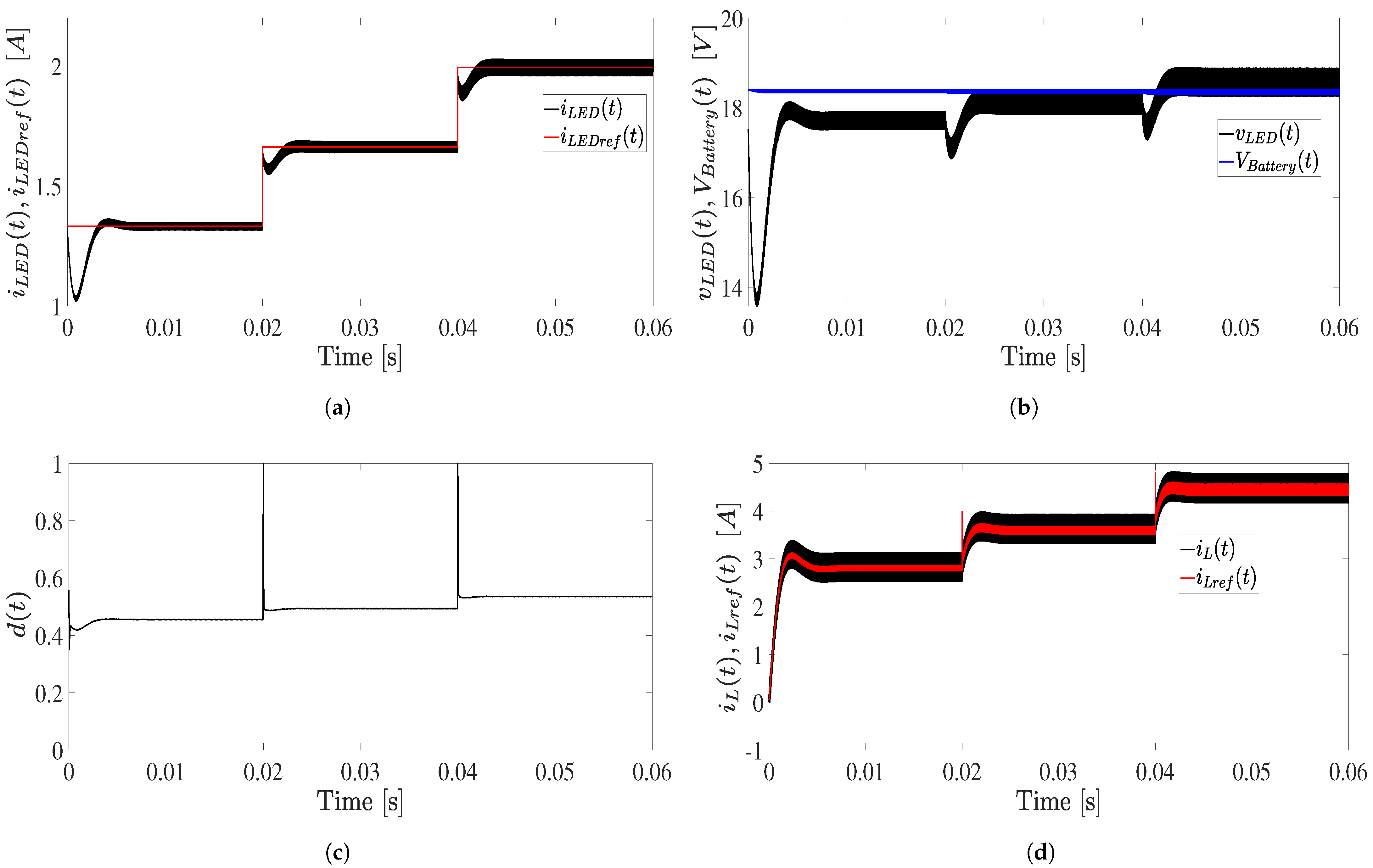
3.3. Test 2: LED Current Control in Buck-Boost Mode

This second test evaluates the commercial 18 V lithium-ion battery model TOOL-486LI-30 under the same LED current and voltage conditions (Figure 11). Consequently, the converter must operate in buck-boost mode.

Figure 11a shows that the behavior is similar to that of the 12 V battery. This is because the references of the iLedref currents are the same. Figure 11b reports that the converter operates as a reducer up to 20 ms. Between 20 ms and 40 ms it operates with a voltage conversion factor close to the unit, and from 40 ms to 60 ms it operates in boost mode. The battery voltage is maintained at 18.4 V, which corresponds to a full charge operation. Figure 11c shows that the duty cycle is not saturated and has a lower value than that of the 12 V battery. It will also have fixed-frequency switching. In Figure 11d, the inductor current $i_L$ follows the reference current $I_{Lref}$ satisfactorily. The system remains fixed-frequency switching and the error in the controlled current is minimal.

3.4. Test 3: LED Current Control in Buck Mode

This third test evaluates the 24 V commercial lead-acid battery UPS-BAT/VRLA-WTR under the same LED current and voltage conditions (Figure 12). Therefore, the converter must operate in buck mode.

Figure 12a reports a behavior similar to that obtained with the 12 V and 18 V batteries, as the current reference of $i_{LEDref}$ is the same. Therefore, the current of the LED $i_{LED}$ and its voltage should be the same, but Figure 12b reports that the buck-boost converter behaves only as a reducer. This checks that the drivers impose the desired current for any voltage value in the battery, thus allowing proper regulation of the LEDs with commercial batteries of various values. Figure 12c shows that the duty cycle has a lower value than when used with 12 and 18 volt batteries, without saturation and with fixed switching frequency. Figure 12d shows the $i_L\left(t\right)$ current, which has a greater ripple than the $i_L\left(t\right)$ current compared to the previous two cases, which is due to the increase in voltage in the battery. In any case, the current $i_L\left(t\right)$ effectively follows the reference $i_{Lref}\left(t\right)$.

Finally, for the three batteries, the system controls the current $i_{LED}$, which maintains the luminous flow at the value desired by the user. In any case, the temperature compensation must be checked (Test 5). The current $i_L\left(t\right)$ is also correctly controlled with the ZAD at a fixed switching frequency with the three batteries.

3.5. Test 4: LED Current Control with Discharged Battery

This fourth test considers a small 12-volt Nickel Metal Hydride battery (CUSTOM-334) with a capacity of 0.4 Ah and an initial state-of-charge of 10% (Figure 13). This configuration produces a fast battery voltage drop, which enables to test the control robustness to changes on the input voltage. Therefore, the same LED current references are adopted.

Figure 13a shows a behavior similar to the previous cases because the system is correctly controlled. In Figure 13b it is observed that the battery voltage starts at 12.04 V and ends at 11.3 V, presenting a reduction of 6% in a time of 6 s. Despite this constant disturbance, the control system ensures the correct regulation of the current of the LEDs according to the reference $i_{LEDref}$.

Figure 13c shows the duty cycle, which behaves similarly to the case of the 12-volt battery, only that as the battery discharges, the duty cycle increases to compensate for the voltage drop at the input. The working cycle at the end of the simulated time of 6 s had to increase 8.5% more than when the battery was charged in Test 1.

Figure 13d shows that the $i_L$ current follows the $i_{L}ref$ reference, only now both have a positive slope due to the discharge of the battery. Both currents have a higher value than in the first test, reaching a final increase of 10.16%.

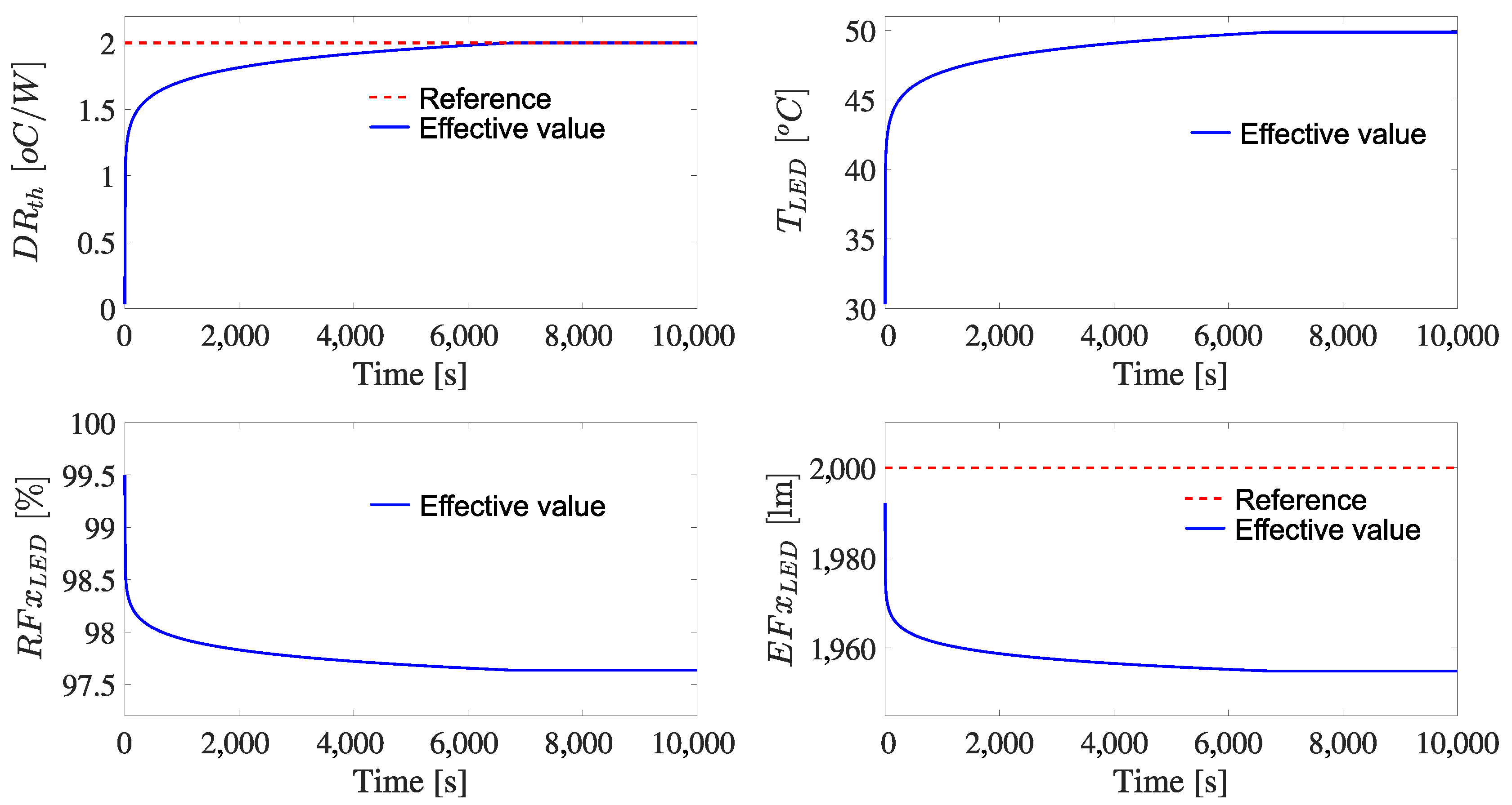
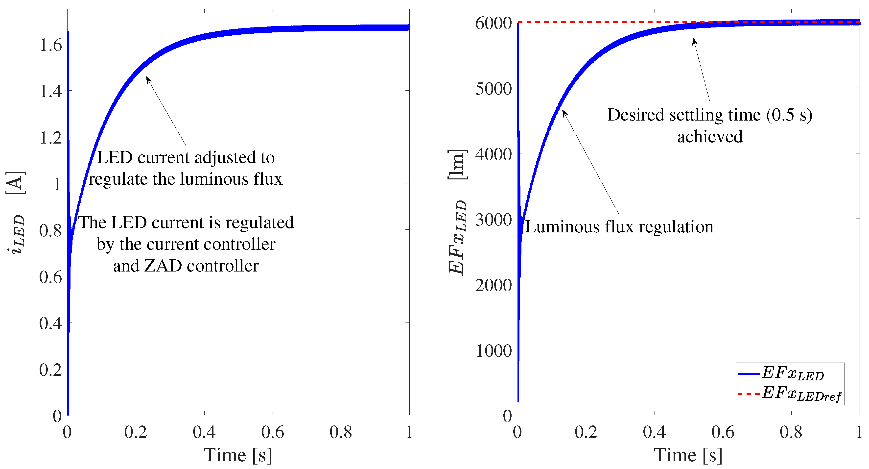
3.6. Test 5: Luminous Flux Regulation

Taking into account that the combined operation of the LED current controller and the ZAD controller imposes the desired current to the LED groups, such a closed-loop system behaves as a current source ensuring $i_{LED}=i_{LEDref}$. Then, the temperature compensator of Figure 9 adjust the reference of the LED current controller $i_{LEDref}$ to ensure the desired luminous flux for any operation temperature. Figure 14 shows the performance of the system under the start-up condition (up to 1 s), where the current of the LED group $i_{LED}$ is adjusted to produce the desired luminous flux $EF{x}_{LEDref}=6000$ lm. Moreover, the figure also confirms that the $P{I}_T$ controller imposes the desired settling time (0.5 s).

A longer simulation is performed to test the system behavior during the thermal stabilization of the LED groups. Figure 15 shows the simulation of the system with an initial reference of the luminous flux equal to $EF{x}_{LEDref}=6000$ lm, where the temperature of the LED group has an increase of 20 °C during 117 min (1 h and 57 min) over the ambient temperature $T_a=30$ °C, reaching a steady state temperature equal to 50 °C. Since such a temperature increase reduces the effective luminous flux $EF{x}_{LED}$ produced by the LED groups, the thermal regulator controller $P{I}_T$ adjusts the current of the LED groups $i_{LED}$ to provide the desired effective luminous flux $EF{x}_{LEDref}$ for any thermal condition. It is satisfactory that the proposed thermal compensator ensures the production of the desired effective luminous flux $EF{x}_{LED}=EF{x}_{LEDref}$ even with a temperature change equal to 66.6% of the initial (ambient) temperature. Then, after 250 min (4 h and 10 min of operation) the reference of the luminous flux is changed to $EF{x}_{LEDref}=5000$ lm, which forces the $P{I}_T$ controller to change the current of the LED groups in order to produce the desired effective luminous flux (5000 lm), also compensating the change in the temperature caused by the reduction in the LEDs power. Figure 15 shows a zoom in this transient between minutes 250 and 251, where the correct current and luminous flux regulations are observed.

Finally, the simulations reported in this subsection confirm the correct regulation of the luminous flux provided by the proposed solution. This is evident from the system performance without the temperature compensator (Figure 8) and with the temperature compensation activated (Figure 15), where the designed temperature compensator successfully regulates the luminous flux for a wide range of temperature conditions. Moreover, the luminous flux can be increased or decreased by changing the reference $EF{x}_{LEDref}$ of the $P{I}_T$ controller, thus providing higher flexibility to the LED system.

4. Conclusions

This paper presented the design of a portable LED lighting system powered by batteries, featuring a combined control strategy based on ZAD and PID controllers:

• This system can adapt the current to maintain constant luminous flux required for reliable portable lighting applications used in outdoor activities.
• The ZAD and PID controllers are capable of switching the MOSFET at a fixed switching frequency as the duty cycle is constant and not saturated. This would reduce switching losses, audible noise in the coil, and subharmonic electromagnetic interferences and chattering.
• The system is able to work even with batteries of different voltages and presents the same behavior in terms of luminosity. The only difference is that, depending on the value of the battery at the input, the system behaves as an elevator or reducer.
• The system works efficiently even if the battery is discharged and maintains the luminous flux constant until it is totally discharged.
• The system can provide uniform illumination during charge and discharge conditions, enhancing usability for outdoor activities, emergency situations, and professional applications. The system is applicable to improve the user experience in activities that require similar illumination over long periods.
• The integration of the temperature compensation loop successfully preserves the effective luminous flux over extended operation times, confirming the controller’s robustness against thermal variations in real use scenarios.
• The joint implementation of the ZAD and PID controllers guarantees precise LED current regulation, enabling smooth tracking of dynamic reference changes with minimal ripple and no overshoot.
• Simulation results confirm that the ZAD-PID control structure is robust against input voltage drops and temperature-induced variations, delivering consistent performance under representative real-world operating conditions.

References

1. Apostolidou, N.; Valsamas, F.; Baros, D.; Loupis, M.; Dasteridis, V.; Kokkinis, C. Innovative energy-recovery unit for the LED-lighting system of heavy-duty vehicles. Clean Technol. 2021, 3, 581–593. [Google Scholar] [CrossRef]
2. Kim, H.C.; Choi, M.C.; Kim, S.; Jeong, D.K. An AC–DC LED driver with a two-parallel inverted buck topology for reducing the light flicker in lighting applications to low-risk levels. IEEE Trans. Power Electron. 2017, 32, 3879–3891. [Google Scholar] [CrossRef]
3. Pinto, R.A.; Cosetin, M.R.; Campos, A.; Dalla Costa, M.A.; do Prado, R.N. Compact emergency lamp using power LEDs. IEEE Trans. Ind. Electron. 2012, 59, 1728–1738. [Google Scholar] [CrossRef]
4. Pulli, T.; Dönsberg, T.; Poikonen, T.; Manoocheri, F.; Kärhä, P.; Ikonen, E. Advantages of white LED lamps and new detector technology in photometry. Light Sci. Appl. 2015, 4, e332. [Google Scholar] [CrossRef]
5. Vieira, J.A.B.; Mota, A.M. Implementation of a stand-alone photovoltaic lighting system with MPPT battery charging and LED current control. In Proceedings of the 2010 IEEE International Conference on Control Applications, Yokohama, Japan, 8–10 September 2010. [Google Scholar]
6. Esteki, M.; Khajehoddin, S.A.; Safaee, A.; Li, Y. LED Systems Applications and LED Driver Topologies: A Review. IEEE Access 2023, 11, 38324–38358. [Google Scholar] [CrossRef]
7. Singh, S.; Bhullar, S. Hardware implementation of auto switching and light intensity control of LED lamps. Balk. J. Electr. Comput. Eng. 2016, 4, 67–71. [Google Scholar] [CrossRef]
8. DiLouie, C. Advanced Lighting Controls: Energy Savings, Productivity, Technology and Applications; River: Gistrup, Denmark, 2021. [Google Scholar]
9. Chepurna, O.; Grebinyk, A.; Petrushko, Y.; Prylutska, S.; Grebinyk, S.; Yashchuk, V.; Matyshevska, O.; Ritter, U.; Dandekar, T.; Frohme, M.; et al. LED-based portable light source for photodynamic therapy. In Proceedings of the Optics in Health Care and Biomedical Optics IX, Hangzhou, China, 21–23 October 2019. [Google Scholar]
10. Bastian, A.; Devara, K.; Ramadhanty, S.; Abuzairi, T. Design of portable emergency lamp utilizing thin film solar cell and inflatable case. E3S Web Conf. 2018, 67, 01019. [Google Scholar] [CrossRef]
11. Restrepo Alvarez, A.F.; Bolivar Chaves, O.F.; Arias, C.M.; Villamil Villar, B.I. Development of a portable lighting system powered by photovoltaic solar energy: Chucheros-Buenaventura community application case. Ing. Compet. 2021, 23, e21010806. [Google Scholar]
12. Matoso, H.M.; Morais, L.M.F.; Cortizo, P.C.; Donoso-Garcia, P.F. Intelligent power LED lighting system with wireless communication. In Proceedings of the IECON 2012—38th Annual Conference on IEEE Industrial Electronics Society, Montreal, QC, Canada, 25–28 October 2012. [Google Scholar]
13. Torrisi, A.; Baggio, F.; Brunelli, D. Visible light communication for intermittent computing battery-less IoT devices. In Lecture Notes in Electrical Engineering; Springer International Publishing: Cham, Switzerland, 2022; pp. 155–163. [Google Scholar]
14. Wu, M.T.; Lin, C.L.; Lin, C.C.; Chung, L.P. Stabilising current driver for high-voltage light-emitting diodes. IET Power Electron. 2014, 7, 1024–1030. [Google Scholar] [CrossRef]
15. Shankar, A.; Vijayakumar, K.; Babu, B.C.; Durusu, A. Smart LED lighting system for energy efficient industrial and commercial LVDC nanogrid powered buildings with BIPV. In Proceedings of the 2020 International Conference on Smart Energy Systems and Technologies (SEST), Istanbul, Turkey, 7–9 September 2020. [Google Scholar]
16. Hariri, A.; Lemaster, J.; Wang, J.; Jeevarathinam, A.S.; Chao, D.L.; Jokerst, J.V. The characterization of an economic and portable LED-based photoacoustic imaging system to facilitate molecular imaging. Photoacoustics 2018, 9, 10–20. [Google Scholar] [CrossRef] [PubMed]
17. Raypah, M.E.; Mahmud, S.; Devarajan, M.; AlShammari, A. Enhancement of luminous flux of InGaAlP-based low-power SMD LEDs using substrates with different thermal resistances. Microelectron. Int. 2020, 38, 6–13. [Google Scholar] [CrossRef]
18. Chen, W.; Fan, J.; Qian, C.; Pu, B.; Fan, X.; Zhang, G. Reliability assessment of light-emitting diode packages with both luminous flux response surface model and spectral power distribution method. IEEE Access 2019, 7, 68495–68502. [Google Scholar] [CrossRef]
19. LUMINUS. MP-5050-240E. Mid Power LED. Product Datasheet. Available online: https://download.luminus.com/datasheets/Luminus_MP5050_240E_Datasheet.pdf (accessed on 15 April 2025).
20. Górecki, K.; Ptak, P.; Janicki, M.; Napieralska, M. Comparison of properties for selected experimental set-ups dedicated to measuring thermal parameters of power LEDs. Energies 2021, 14, 3240. [Google Scholar] [CrossRef]
Figure 1. General diagram of the system that represents the model of the buck-boost converter with LED current and inductor current controls.
Asi 08 00059 g001
Figure 2. Model that represents the parameters of the buck-boost converter.
Asi 08 00059 g002
Figure 3. Equivalent circuit of the closed-loop ZAD controller.
Asi 08 00059 g003
Figure 4. (a) Comparison of the exact and approximate models, and (b) controller performance with both exact and approximate models.
Asi 08 00059 g004
Figure 5. LED current, voltage, and luminous flux relations.
Asi 08 00059 g005
Figure 6. LED relative luminous flux and effective luminous flux vs. temperature.
Asi 08 00059 g006
Figure 7. Dynamic behavior of the thermal resistance.
Asi 08 00059 g007
Figure 8. Dynamic LED group simulation with constant current.
Asi 08 00059 g008
Figure 9. Block diagram of the temperature compensator.
Asi 08 00059 g009
Figure 10. Results of the LED current control in boost mode with a 12-volt battery.
Asi 08 00059 g010
Figure 11. Results for the LED current control in buck-boost mode with a 18-volt battery.
Asi 08 00059 g011
Figure 12. Results for the LED current control in buck mode with a 24-volt battery.
Asi 08 00059 g012
Figure 13. Results for the LED current control with a discharged 12-volt battery.
Asi 08 00059 g013
Figure 14. Regulation of the luminous flux adjusting the LED group current.
Asi 08 00059 g014
Figure 15. System operation during the LED temperature stabilization.
Asi 08 00059 g015