

Influence of Voltage Rising Time on the Characteristics of a Pulsed Discharge in Air in Contact with Water: Experimental and 2D Fluid Simulation Study


Abstract
:1. Introduction
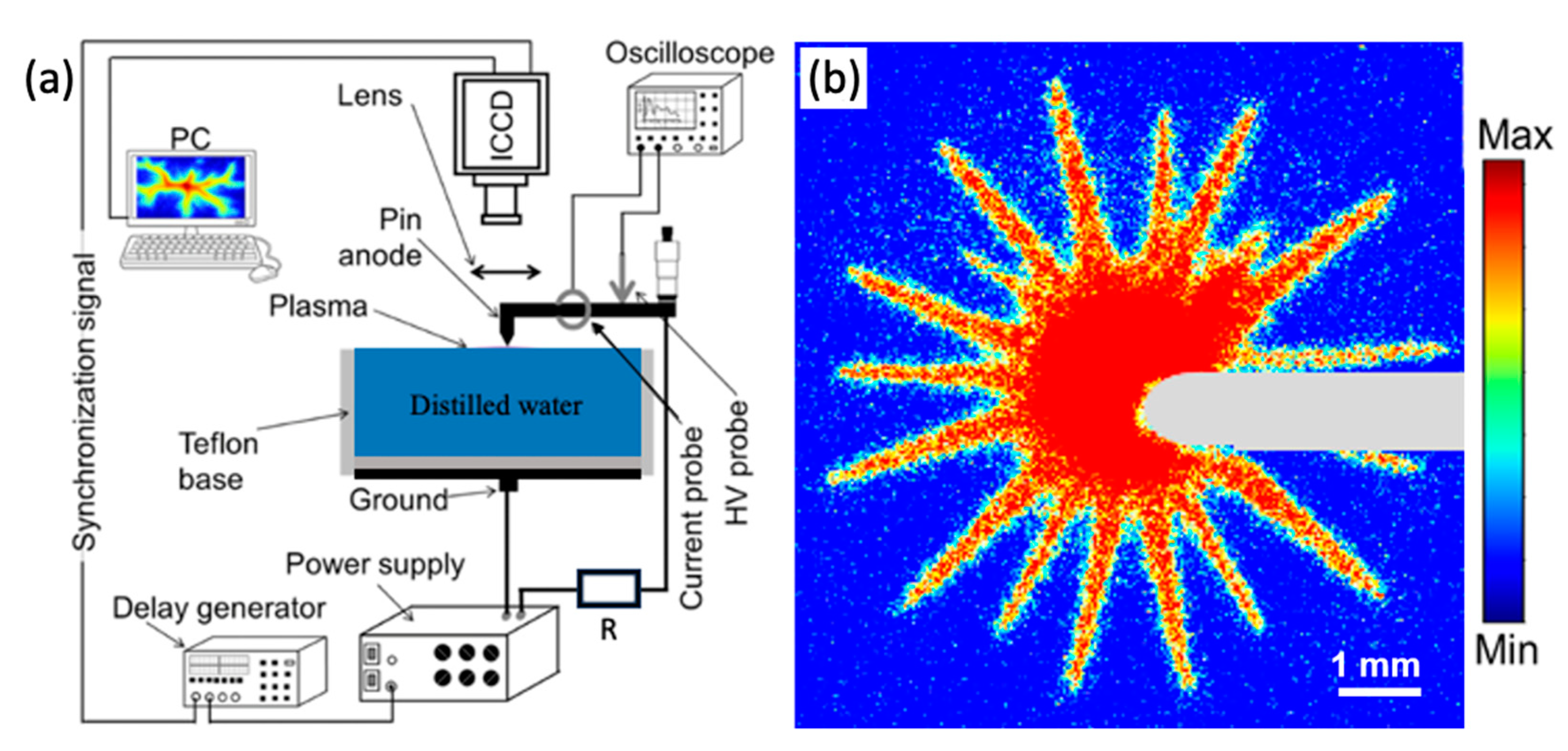
2. Experimental Conditions
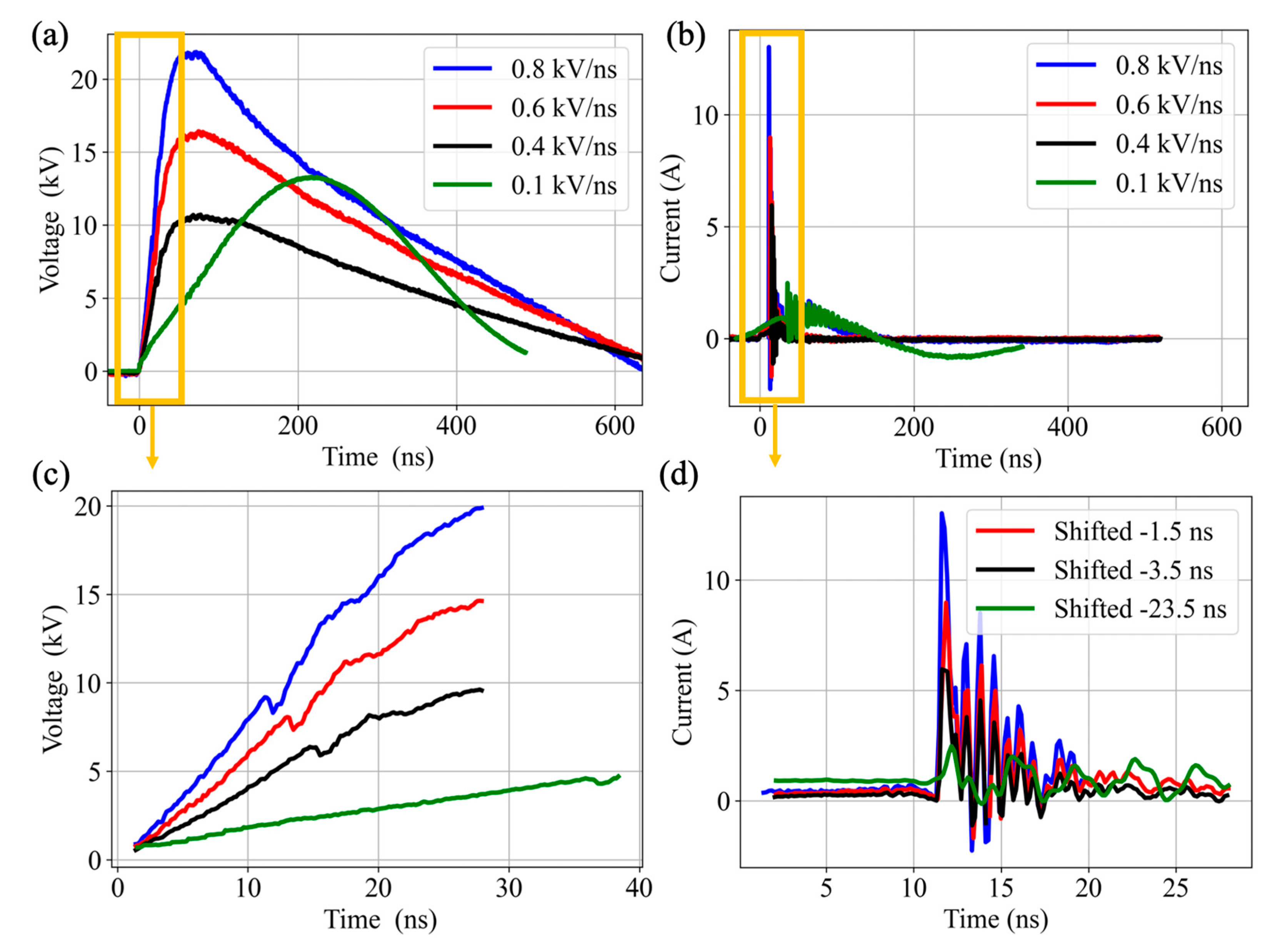
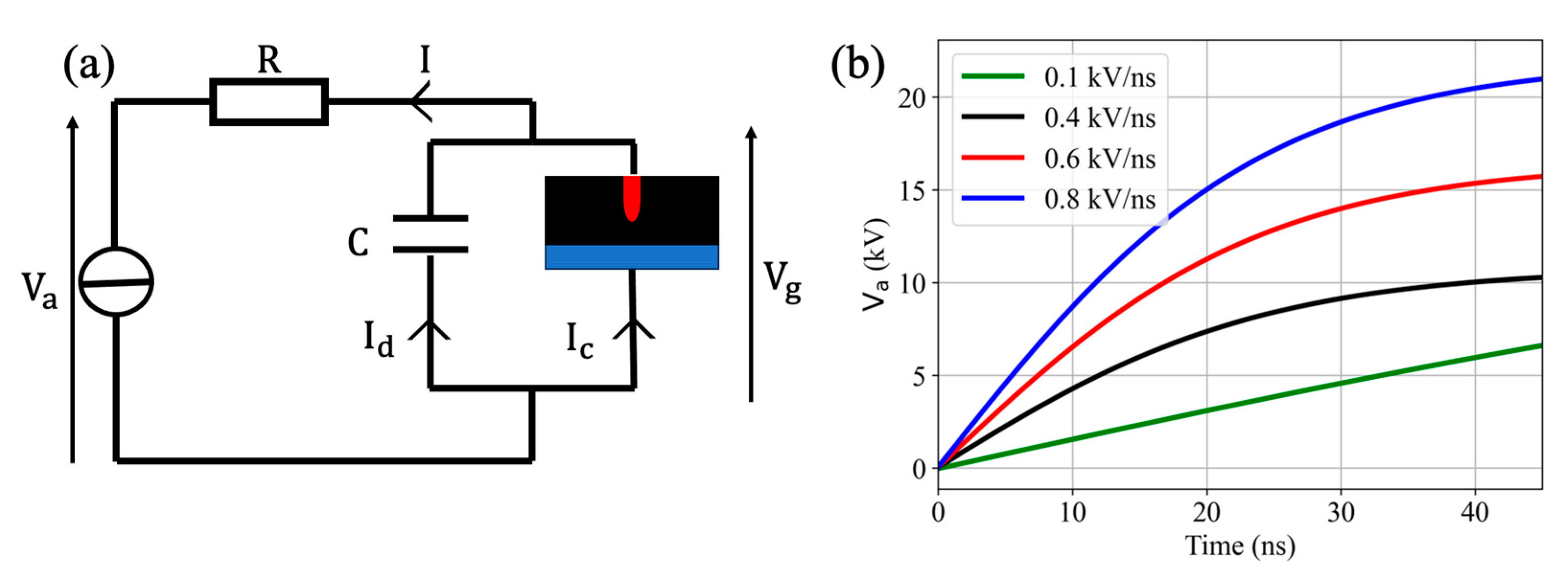
2.1. Electrical Characterization
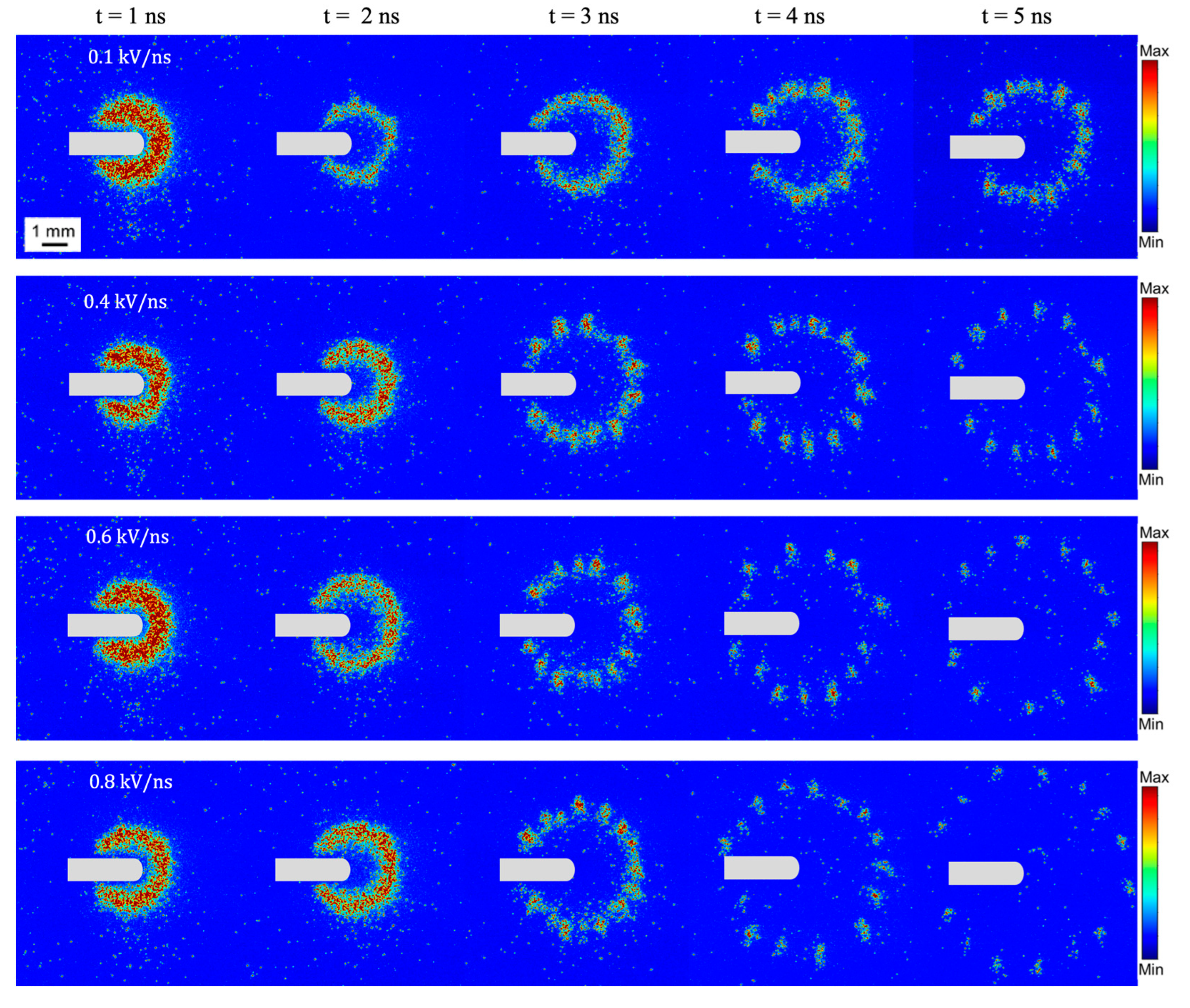
2.2. ICCD Imaging
3. Numerical Simulation
3.1. Discharge Model Equations, Boundary Conditions, and Computational Domain
- From to , uniform grid with ;
- From to , uniform grid with ;
- From to , non-uniform grid with a geometric expansion up to ;
- From to , uniform grid with ;
- From to , non-uniform grid with a geometric expansion up to m;
- From to , non-uniform grid with a geometric expansion up to .
3.2. Simulation Results
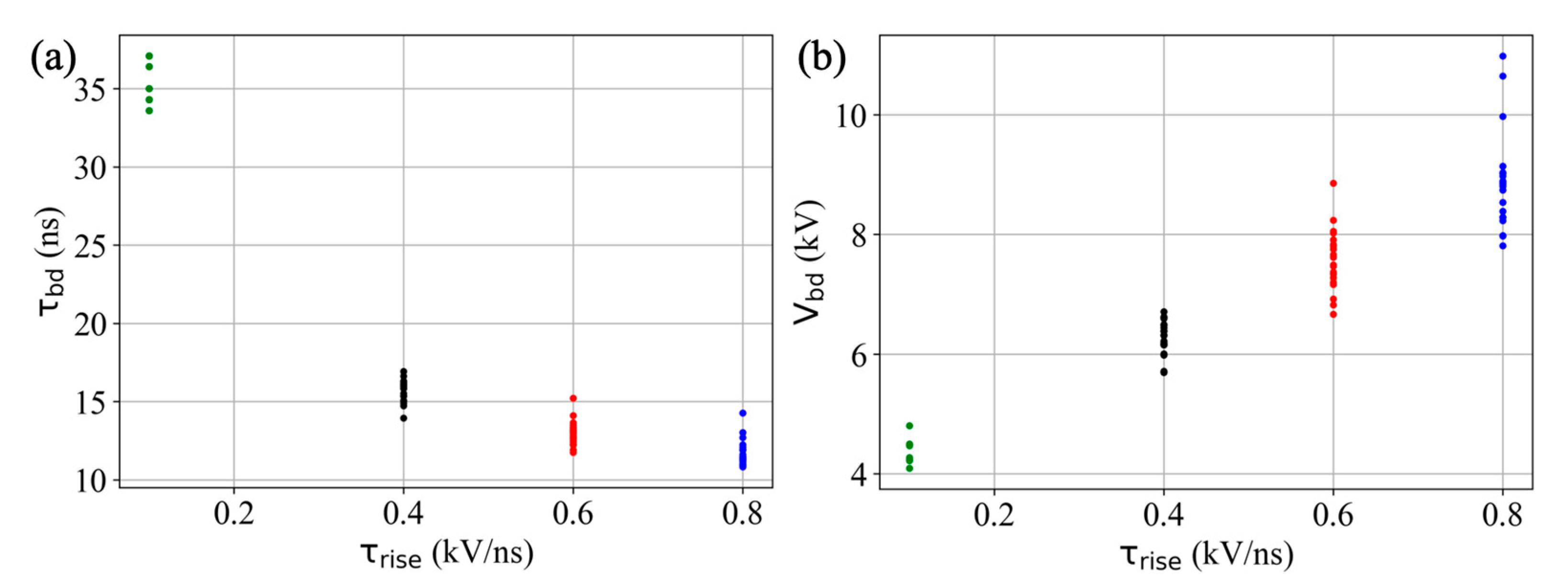
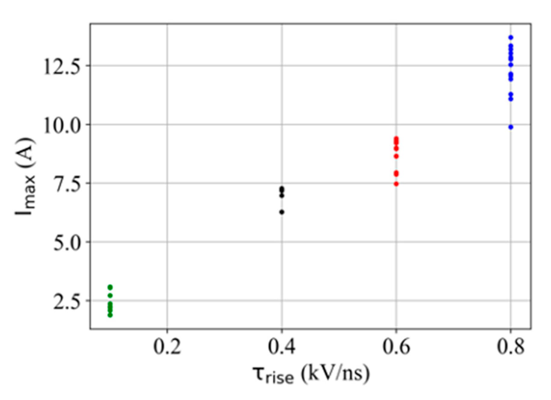
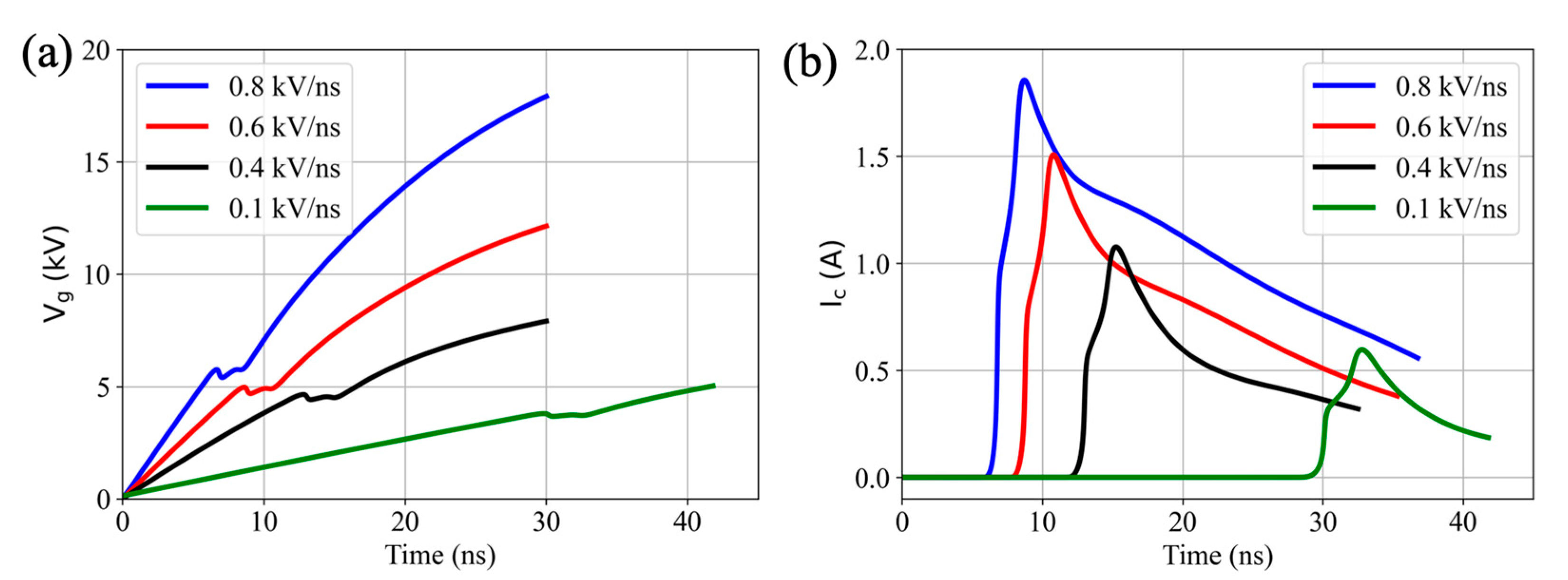
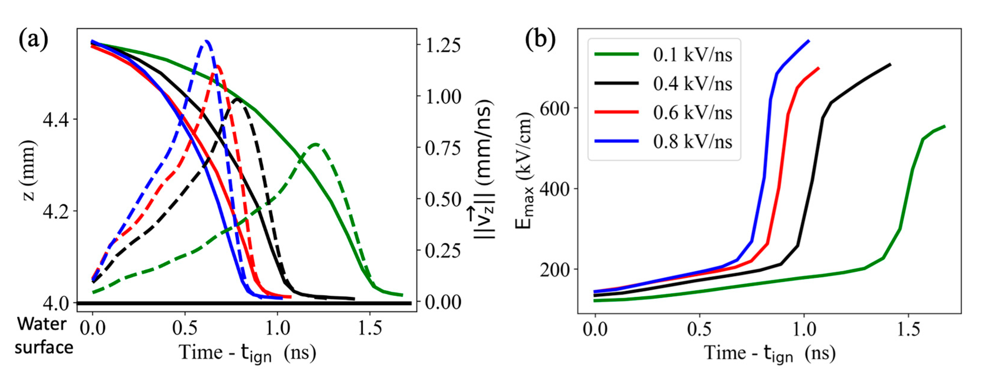
3.2.1. Electrical Results
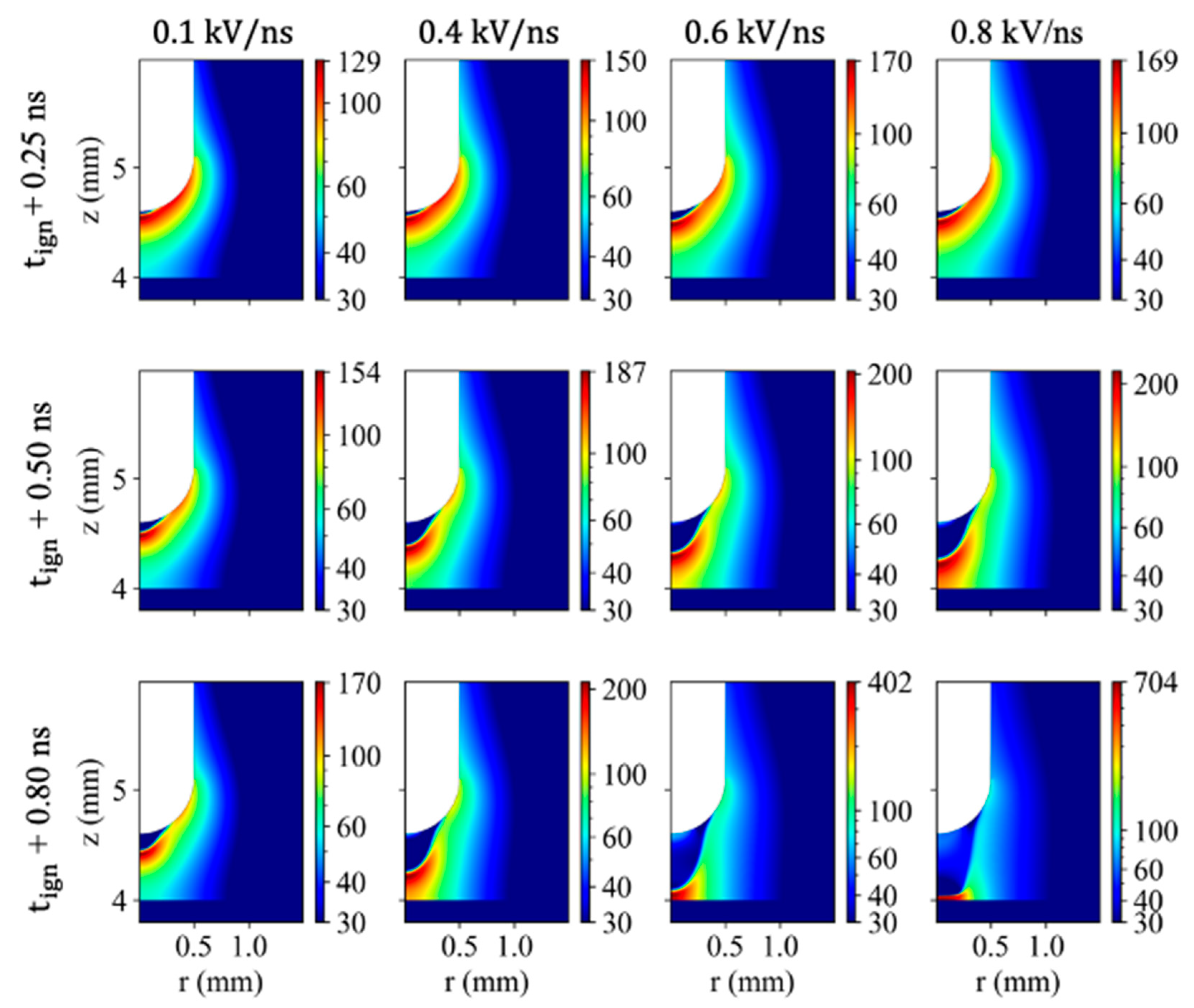
3.2.2. Vertical Propagation
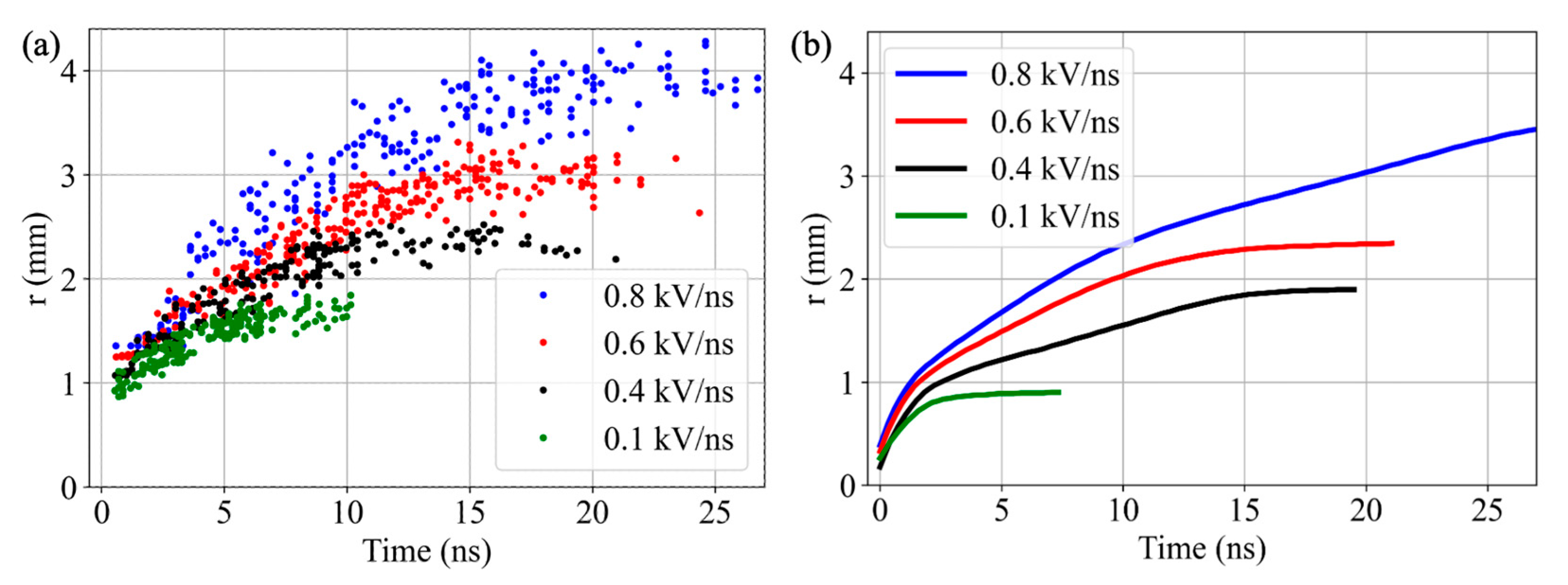
3.2.3. Radial Propagation
4. Discussion
4.1. Impact of on Discharge Ignition
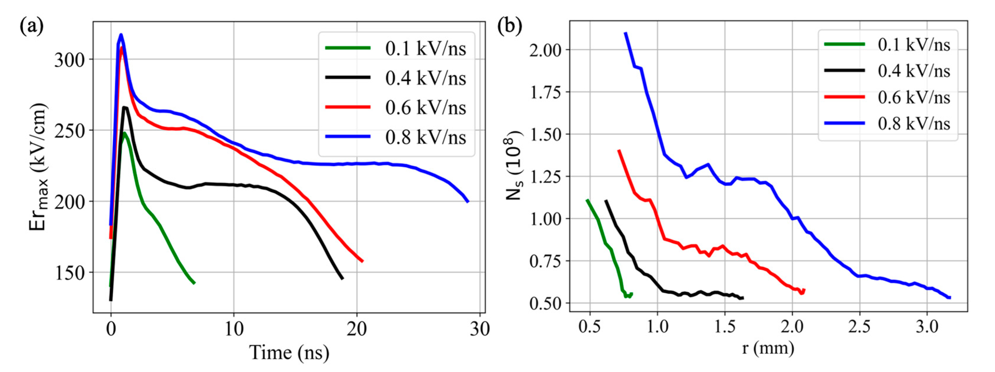
4.2. Impact of on the E-Field and during the Radial Propagation
5. Conclusions
Author Contributions
Funding
Data Availability Statement
Conflicts of Interest
References
- Kulikovsky, A.A. Analytical model of positive streamer in weak field in air: Application to plasma chemical calculations. IEEE Trans. Plasma Sci. 1998, 26, 1339–1346. [Google Scholar] [CrossRef]
- Li, C.; Teunissen, J.; Nool, M.; Hundsdorfer, W.; Ebert, U. A comparison of 3D particle, fluid and hybrid simulations for negative streamers. Plasma Sources Sci. Technol. 2012, 21, 055019. [Google Scholar] [CrossRef]
- Teunissen, J. Improvements for drift-diffusion plasma fluid models with explicit time integration. Plasma Sources Sci. Technol. 2020, 29, 015010. [Google Scholar] [CrossRef]
- Montijn, C.; Ebert, U. Diffusion correction to the Raether-Meek criterion for the avalanche-to-streamer transition. J. Phys. D Appl. Phys. 2006, 39, 2979–2992. [Google Scholar] [CrossRef]
- Rezaei, F.; Vanraes, P.; Nikiforov, A.; Morent, R.; De Geyter, N. Applications of plasma-liquid systems: A review. Materials 2019, 12, 2751. [Google Scholar] [CrossRef]
- Bagheri, B.; Teunissen, J.; Ebert, U.; Becker, M.M.; Chen, S.; Ducasse, O.; Eichwald, O.; Loffhagen, D.; Luque, A.; Mihailova, D.; et al. Comparison of six simulation codes for positive streamers in air. Plasma Sources Sci. Technol. 2018, 27, 095002. [Google Scholar] [CrossRef]
- Laroussi, M. Plasma Medicine: A Brief Introduction. Plasma 2018, 1, 47–60. [Google Scholar] [CrossRef]
- Kim, M.C.; Yang, S.H.; Boo, J.-H.; Han, J.G. Surface treatment of metals using an atmospheric pressure plasma jet and their surface characteristics. Surf. Coat. Technol. 2003, 174, 839–844. [Google Scholar] [CrossRef]
- Celestin, S.; Allegraud, K.; Canes-Boussard, G.; Leick, N.; Guaitella, O.; Rousseau, A. Patterns of plasma filaments propagating on a dielectric surface. IEEE Trans. Plasma Sci. 2008, 36, 1326–1327. [Google Scholar] [CrossRef]
- Meyer, H.K.H.; Marskar, R.; Mauseth, F. Evolution of positive streamers in air over non-planar dielectrics: Experiments and simulations. Plasma Sources Sci. Technol. 2022, 31, 114006. [Google Scholar] [CrossRef]
- Eichwald, O.; Ducasse, O.; Dubois, D.; Abahazem, A.; Merbahi, N.; Benhenni, M.; Yousfi, M. Experimental analysis and modelling of positive streamer in air: Towards an estimation of O and N radical production. J. Phys. D Appl. Phys. 2008, 41, 23. [Google Scholar] [CrossRef]
- Li, X.; Sun, A.; Zhang, G.; Teunissen, J. A computational study of positive streamers interacting with dielectrics. Plasma Sources Sci. Technol. 2020, 29, 065004. [Google Scholar] [CrossRef]
- Bourdon, A.; Péchereau, F.; Tholin, F.; Bonaventura, Z.; Study, Z.B. Study of the electric field in a diffuse nanosecond positive ionization wave generated in a pin-to-plane geometry in atmospheric pressure air. J. Phys. D Appl. Phys. 2021, 54, 075204. [Google Scholar] [CrossRef]
- Konina, K.; Raskar, S.; Adamovich, I.V.; Kushner, M.J. Atmospheric pressure plasmas interacting with wet and dry microchannels: Reverse surface ionization waves. Plasma Sources Sci Technol. 2024, 33, 015002. [Google Scholar] [CrossRef]
- Höft, H.; Kettlitz, M.; Brandenburg, R. The role of a dielectric barrier in single-filament discharge over a water surface. J. Appl. Phys. 2021, 129, 043301. [Google Scholar] [CrossRef]
- Yang, X.; Wang, W.; Wang, X.; Du, Y.; Meng, Y.; Wu, K. Experimental study of transient surface charging during dielectric barrier discharges in air gap in needle-to-plane geometry. J. Phys. D Appl. Phys. 2023, 56, 465202. [Google Scholar] [CrossRef]
- Herrmann, A.; Margot, J.; Hamdan, A. Influence of voltage and gap distance on the dynamics of the ionization front, plasma dots, produced by nanosecond pulsed discharges at water surface. Plasma Sources Sci. Technol. 2022, 31, 045006. [Google Scholar] [CrossRef]
- Hamdan, A.; Diamond, J.; Stafford, L. Time-resolved imaging of pulsed positive nanosecond discharge on water surface: Plasma dots guided by water surface. Plasma Sources Sci. Technol. 2020, 29, 115017. [Google Scholar] [CrossRef]
- Höft, H.; Becker, M.M.; Loffhagen, D.; Kettlitz, M. On the influence of high voltage slope steepness on breakdown and development of pulsed dielectric barrier discharges. Plasma Sources Sci. Technol. 2016, 25, 064002. [Google Scholar] [CrossRef]
- Yoon, S.Y.; Jeon, H.; Yi, C.; Park, S.; Ryu, S.; Kim, S.B. Mutual interaction between plasma characteristics and liquid properties in AC-driven pin-to-liquid discharge. Sci. Rep. 2018, 8, 12037. [Google Scholar] [CrossRef]
- Herrmann, A.; Margot, J.; Hamdan, A. Experimental and 2D fluid simulation of a streamer discharge in air over a water surface. Plasma Sources Sci. Technol. 2024, 33, 025022. [Google Scholar] [CrossRef]
- Merciris, T.; Valensi, F.; Hamdan, A. Determination of the Electrical Circuit Equivalent to a Pulsed Discharge in Water: Assessment of the Temporal Evolution of Electron Density and Temperature. IEEE Trans. Plasma Sci. 2020, 48, 3193–3202. [Google Scholar] [CrossRef]
- Zhang, Q.Z.; Zhang, L.; Yang, D.Z.; Schulze, J.; Wang, Y.N.; Bogaerts, A. Positive and negative streamer propagation in volume dielectric barrier discharges with planar and porous electrodes. Plasma Process. Polym. 2021, 18, e2000234. [Google Scholar] [CrossRef]
- Nijdam, S.; Teunissen, J.; Ebert, U. The physics of streamer discharge phenomena. Plasma Sources Sci. Technol. 2020, 29, 103001. [Google Scholar] [CrossRef]


Disclaimer/Publisher’s Note: The statements, opinions and data contained in all publications are solely those of the individual author(s) and contributor(s) and not of MDPI and/or the editor(s). MDPI and/or the editor(s) disclaim responsibility for any injury to people or property resulting from any ideas, methods, instructions or products referred to in the content. |
© 2024 by the authors. Licensee MDPI, Basel, Switzerland. This article is an open access article distributed under the terms and conditions of the Creative Commons Attribution (CC BY) license (https://creativecommons.org/licenses/by/4.0/).
Share and Cite
Herrmann, A.; Margot, J.; Hamdan, A. Influence of Voltage Rising Time on the Characteristics of a Pulsed Discharge in Air in Contact with Water: Experimental and 2D Fluid Simulation Study. Plasma 2024, 7, 616-630. https://doi.org/10.3390/plasma7030032
Herrmann A, Margot J, Hamdan A. Influence of Voltage Rising Time on the Characteristics of a Pulsed Discharge in Air in Contact with Water: Experimental and 2D Fluid Simulation Study. Plasma. 2024; 7(3):616-630. https://doi.org/10.3390/plasma7030032
Chicago/Turabian StyleHerrmann, Antoine, Joëlle Margot, and Ahmad Hamdan. 2024. "Influence of Voltage Rising Time on the Characteristics of a Pulsed Discharge in Air in Contact with Water: Experimental and 2D Fluid Simulation Study" Plasma 7, no. 3: 616-630. https://doi.org/10.3390/plasma7030032
APA StyleHerrmann, A., Margot, J., & Hamdan, A. (2024). Influence of Voltage Rising Time on the Characteristics of a Pulsed Discharge in Air in Contact with Water: Experimental and 2D Fluid Simulation Study. Plasma, 7(3), 616-630. https://doi.org/10.3390/plasma7030032