Instability of a Moving Bogie: Analysis of Vibrations and Possibility of Instability in Subcritical Velocity Range

Abstract

This paper analyzes vibrations induced by a moving bogie passing through a single-layer railway track model. The emphasis is placed on the possibility of unstable behavior in the subcritical velocity range. All results are presented in dimensionless form to encompass a wide range of possible scenarios. The results are obtained semi-analytically, however, the only numerical step involves solving the roots of polynomial expressions. No numerical integration is used, allowing for the straightforward solution of completely undamped scenarios, as damping is not required for numerical stability. The vibration shapes are presented in the time domain in closed form. It is concluded that increased foundation damping worsens the situation. However, in general, the risk of instability in the subcritical velocity range for a moving bogie is lower than that of two moving masses, particularly for higher mass moments of inertia of the bogie bar and primary suspension damping. The study also examines how the results change when a Timoshenko-Rayleigh beam is considered instead of an Euler-Bernoulli beam. Although some cases may appear academic, it is demonstrated that instability in the supercritical velocity range cannot be assumed to be guaranteed.

1. Introduction

One effective way to combat climate change and reduce the carbon footprint is to prioritize rail transport over road transport. This naturally necessitates an increase in railway network capacity by enhancing travel velocity, the number of trains, and axle loads. These increased demands emphasize the importance of ensuring passenger safety and comfort. The upper limit for travel velocity is typically derived from the critical velocity, which, in this context, corresponds to the critical velocity of a moving force. This velocity equals the lowest wave propagation velocity in the supporting structure, resulting from the dynamic interaction of all involved components, and can be referred to as the critical velocity for resonance.

Another commonly used indicator for ensuring safe train passage is the receptance curve, which, however, only indicates the natural frequencies of the supporting structure. The frequencies that cause unstable behavior cannot be identified using receptance curves, as they depend on the mass and velocity of the moving object. Therefore, it is necessary to study the transient vibrations caused by the moving vehicle and the associated so-called induced frequencies, which can determine whether the motion will be stable or unstable. Nevertheless, the problem of instability has often been overlooked, as it was shown that a single moving mass or oscillator can exhibit unstable behavior only in the supercritical velocity range. Since this region is a priori excluded from track design, instability has not been considered a critical issue.

However, the dynamic interaction of two moving proximate masses can lead to a different scenario, one that surprisingly worsens with increased foundation damping. Such cases have already been identified in the author’s previous works.

The study of moving load problems remains a highly active topic in transportation engineering, particularly in rail and road transport. Various simplifications have been introduced to improve computational efficiency and present results in a more compact form suitable for optimization and sensitivity analyses. These simplifications apply to the supporting structure, the moving vehicle, or both, depending on the problem being investigated. In addition to analyzing the influence of several parameters on dynamic performance, key topics of interest include the critical velocity for resonance, the critical frequency for resonance, instability, and the dynamic interaction of proximate inertial objects.

Typical simplifications at the level of the supporting structure have led to layered models consisting of beams, point masses, and spring-damper elements. These models are widely used due to their simplicity and computational efficiency. Such simplified models, along with simplified vehicle models, are used in both practical and theoretical studies. The applicability of the three-layer model in railway applications is analyzed in [1], while an overview of the features of one-, two-, and three-layer models is provided in [2]. Notably, these simplified models have proven adequate for modeling several railway dynamics issues, as demonstrated by other researchers, including in classical works [3,4]. Other works dealing with vehicle–track dynamic interaction modeling include [5,6,7,8,9,10,11,12,13], further demonstrating the usefulness of simplified models. A classification of layered models is introduced in [4], with validation against experimental results provided in [14]. Studies aimed at defining the properties of such models consider the ballast pyramid model, as referenced in [15,16], and the Saller assumption from 1932, which can be consulted in [17]. The pyramid model is further detailed in [18] under the name “stress cone model”, where it is used to define vertical ballast stiffness and identify dynamically activated ballast mass. Further improvements involve the superposition of cones between adjacent sleepers, i.e., in the longitudinal direction [14].

Numerous research studies have been conducted over the past decades; thus, this review primarily focuses on the most recent publications.

In [19], a critical discussion on developments in the field of the dynamic response of rigid road pavements to moving vehicles is presented. Rigid pavements consist of an elastic concrete plate or jointed plates resting on a supporting foundation. Similar models are also used in railway engineering, albeit with different parameters. The supporting medium can be modeled as a system of spring-damper elements or as a homogeneous or layered half-plane/space with infinite or finite depth. The paper summarizes works in which the material behavior of the subgrade layers is considered isotropic, anisotropic, viscoelastic, poroelastic, or inelastic. In [20], the same authors provide a more detailed review of both rigid and flexible pavements. These works simulate vehicles using either constant concentrated forces or distributed forces over a finite line/area, omitting their inertial effects and, consequently, the possibility of instability. In [21], a plane strain model is used to analyze instability issues in the moving mass problem.

In [22], although the study focuses on road pavements, the guiding structure model corresponds to a one-layer model commonly used in railway applications. The model is traversed by a two-mass oscillator with a contact spring-damper element, a configuration frequently encountered in railway applications. Harmonic roughness of the roadway is considered, but neither instability nor critical velocity is analyzed. Since only a single contact point is involved, the dynamic interaction of proximate objects cannot be observed. The study primarily analyzes the effects of foundation nonlinearity using the Adomian decomposition method. Moving coordinates are implemented, and results are limited to the steady-state response, as only a single Fourier transform is applied. This approach effectively removes the inertial effects of the moving object. The study finds that there is a critical value for nonlinear stiffness, which increases with vehicle velocity and foundation damping.

Regarding railway applications, the nonlinearity of the supporting structure is analyzed in [23]. A two-layer model is implemented, and a simplified vehicle model is used. A novel nonlinear stiffness model is developed to comprehensively characterize ballast properties, incorporating displacement-dependent stiffness, frequency-dependent stiffness, hysteresis, and time/space-varying features. The model is validated using experimental measurements by processing ground-penetrating radar signals with the adaptive optimal kernel time–frequency representation method.

Moving force problems are simpler than moving mass problems, particularly for finite-length supporting structures, where analytical solutions exist and can be formalized using modal expansion. However, a relatively recent study [24] still analyzes this problem for a double-beam structure, focusing on the effects of various boundary conditions. Although the motion of a mass on finite Euler-Bernoulli beams without an elastic foundation and damping is a classical problem addressed by numerous researchers, new insights and results continue to emerge, as shown in [25]. Furthermore, in [26], a new equivalent lumped parameter model is proposed to describe the vibrations of simply supported beams without an elastic foundation under moving force action. This classical problem has a fully analytical solution. In [27], vibrations of a similar structure subjected to a moving mass are solved using the Green’s function method to analyze the effects of boundary conditions, mass velocity, and its ratio with respect to the beam mass.

More practical studies typically address railway line degradation, such as transition zones, rail corrugation, maintenance optimization, and potential failures. For example, in [28], the effect of temperature on concrete cracking in ballastless lines is analyzed, while in [29] the failure of railway vehicle suspension dampers is examined using cross-correlation analysis of bogie accelerations.

Regarding transition zones, it is well known that a sudden change in the vertical stiffness of railway tracks increases dynamic loads and leads to numerous defects in ballasted tracks. The main geometric parameters of the approach slab for short-span bridges were optimized in [30]. A finite element model was developed and subjected to a series of moving forces. The model was validated using field measurements obtained through a laser/camera-based measuring technique. The geometric sensitivity analysis results indicate that rail and ballast displacements can be significantly reduced by employing a geometrically optimized approach slab along the transition zone of a railway bridge.

In [31], a recently proposed revolutionary design aimed at mitigating the negative effects of transition zones is evaluated under extreme conditions. This transition structure, called SHIELD (Safe Hull Inspired Energy Limiting Design), was designed to reverse propagating waves by inverting the shape of the embankment zone, thereby directing wave energy toward the foundation instead of upwards, where it could damage the railroad. The study found that this novel design effectively reduces dynamic amplifications and ensures a smooth distribution of deformation energy across subcritical, critical, and supercritical velocity regimes in both travel directions. This results in a more uniform traffic-induced degradation along the longitudinal direction.

Transition zones are directly linked to the floating sleeper phenomenon, for which a novel modeling approach is presented in [32]. This study provides an accurate mathematical model with a minimal number of degrees of freedom, supported by extensive field measurements of a railway track. Although the observed phenomenon is highly complex, a simplified one-degree-of-freedom mathematical model has been found sufficiently accurate for its characterization.

Regarding rail corrugation, a new hypothesis for the formation process of short-pitch rail corrugation is proposed in [33]. A dynamic finite element (FE) wheel-track model is used to verify the hypothesis by replicating the initiation and consistent growth of corrugation. The FE model consists of discrete elements, similar to other works employing semi-analytical or analytical solutions. The supporting structure is represented as a two-layer model extended to three dimensions, with rail pads and the foundation (corresponding solely to the ballast layer) modeled using spring-damper elements acting in three directions. The wheelset and rails are detailed using 3D elements, while the remaining vehicle mass is lumped and placed above the primary suspension. The study finds that longitudinal compression modes are responsible for corrugation initiation, and the proposed mechanism successfully explains field observations. The FE model is validated using a downscaled V-Track test rig in [34].

Transition zones are also related to transition radiation. In this context, Refs. [35,36] are worth mentioning. Additionally, Ref. [37] provides an insightful analysis using a one-layer model, with adequate justification regarding how results obtained from simplified models should be interpreted. It is well known that the one-layer model significantly overestimates the critical velocity of a railway track. In light of this, the results should be understood qualitatively, as the ratio of train velocity to critical velocity is more relevant than the absolute values of these quantities.

In terms of maintenance, ballast tamping remains the most common method for restoring ballast bed geometry. In [38], a novel test device is introduced that enables real-time evaluation of the mechanical properties of ballast beds, which is essential for optimizing tamping efforts in railway maintenance. The evaluation is based on measuring the impact force on the tamper, and the results are validated numerically using a coupled model where the ballast is represented using the discrete element method.

In [39], a closed-form solution is derived using the residue theorem and Green’s function for the dynamic response of an infinite beam resting on a viscoelastic foundation subjected to a harmonic moving load. However, closed-form results have already been presented in [40]. In [39], these results are used to determine the most appropriate span length of an analogous finite beam to best approximate the deflection of an infinite beam for practical applications. As demonstrated in [41], this can be problematic for a constant moving force, and a solution is proposed in that work. However, for a moving inertial load, no solution is provided, despite previous studies by the author of this paper, where validation was always performed on finite beams. The only precaution taken was to initiate the load slightly farther from the support, as explained in [42]. When considering initial conditions, this distance must be extended to ensure that the entire relevant portion of the initial shape [43] is contained within the beam at time zero.

Similar models are discussed in [44], but only steady-state vibrations are analyzed, thereby eliminating the possibility of instability. However, the model is more detailed, incorporating rail roughness and contact springs. Rail corrugation effects are also considered in [45].

Additionally, other works analyze the limitations of classical beam theories [46,47,48], large deformations [49], non-uniform motion of an inertial object [50], and railway tracks beyond classical ballasted ones [51].

The stability of a moving inertial object on an elastic structure in railway applications has been investigated using various representations of the vehicle (moving object) and the track (supporting or guiding structure). Simplified vehicle models include a moving mass [52,53], a two-mass oscillator [40,54], and a three-mass oscillator [55]. These models have only one contact point, meaning dynamic interaction cannot be observed, unlike models considering two moving masses [42,56] or a sequence of two-mass oscillators [57,58,59,60]. A more complex vehicle model can also be employed for stability analysis [61]. The guiding structure is modeled using an Euler-Bernoulli infinite beam on a continuous foundation with one elastic layer [53,55,56,57], two layers [42,62], or three layers [2]. Alternatively, the Timoshenko beam can be used instead of the Euler-Bernoulli beam [56,63]. To account for the influence of sleeper bays, an infinite beam model with discrete supports should be considered for railway tracks [64].

The instability of a moving bogie has been analyzed in previous studies, but none have provided complete vibration shapes, closed-form time-domain analytical solutions, alternatives to the D-decomposition method, validation on finite beams, etc. A pioneering study on railway vehicle stability [65] focused on lateral stability, a topic not covered in this paper, which only examines vertical vibrations. However, the model presented here is similar to the one in that study. The model in [65] incorporates rail irregularities but restricts calculations to forced steady-state vibrations induced by harmonic irregularities. Since transient vibrations are not evaluated, instability caused by anomalous Doppler waves in the beam cannot be identified. In [66], the influence of track gauge and rail irregularities on hunting motion instability is analyzed, which is beyond the scope of this paper’s plane model.

The instability of a moving bogie passing through a single-layer model is examined in [67] from multiple perspectives, including a comparison with a moving oscillator and an analysis of critical primary suspension stiffness. In [68], the authors investigate how a more complex foundation structure affects critical stiffness values. However, only isolated values are provided without detailed comparison to [67]. The critical velocity for resonance differs significantly from that of the one-layer model, requiring a different approach to comparison. The same reference input data for the moving bogie as in [67] are used. Due to the large distance between the wheels, the dynamic interaction between them is suppressed, and instability is only detectable for realistic values in the supercritical velocity range. In [69], more complex moving objects are introduced, but results are limited to a few discrete values of critical primary suspension stiffness. The effects of foundation damping and instability in the subcritical velocity range are not addressed in these studies.

The present paper analyzes a moving bogie to clarify the possibility of instability in the subcritical velocity range. The results are presented as analytically as possible, building upon previous developments in [40,53,56] while avoiding the Green’s function method used by several other researchers due to its limitations. The primary drawback of this method is its dependence on numerical integration, which necessitates the introduction of damping for numerical stability. When damping is introduced, true resonance cannot be precisely identified or analytically determined. A comparison of both methods is available in [70]. Recent research has shown that the instability of two proximate moving masses on a layered track model can occur in the subcritical velocity range [42,56], contradicting the conventional belief that unstable velocities always exceed the lowest critical velocity for resonance. While instability is mathematically impossible for a single moving object with one contact point, it can occur for multiple moving objects due to dynamic interaction. Additionally, increased foundation damping unexpectedly worsens the situation. This paper’s novel contribution is analyzing how this behavior changes when the moving masses are combined into a bogie, a more realistic representation. The study aims to identify scenarios in which bogie instability occurs in the subcritical velocity range and determine the parameters contributing to this unexpected phenomenon, as well as those that push instability into the expected supercritical velocity range.

The paper is organized as follows. Section 2 describes the model along with the governing equations and their solutions, utilizing the new method from [53] to present the results in closed-form formulas. Dimensionless parameters are introduced to cover a broad range of possible scenarios, allowing the results to be applied without the need for recalculations. Section 3, which presents the results, is divided into several parts. It first defines the induced frequencies and then validates the results through analysis on finite beams. The effects of transitioning from the Euler-Bernoulli beam to the Timoshenko-Rayleigh beam are then examined, followed by a presentation of selected cases along with their corresponding induced frequencies. Next, the conditions leading to instability in the subcritical velocity range for two moving proximate masses are summarized and compared with those for a two-axle bogie. The influence of suspension damping, beam theory, and other input parameters is subsequently analyzed. The results section concludes with a comparison to other published works, particularly [67]. Additional cases are provided in Appendix A due to the length of the paper. Finally, the paper concludes with a discussion of the results, followed by the conclusions.

2. Description of the Model and Governing Equations

The model considered in the present paper is depicted in Figure 1. In part (a), two proximate masses pass through the one-layer model, while in part (b), a single bogie moves across the model. The model consists of a beam characterized by its bending stiffness $EI$ and mass per unit length $m$, following the Euler-Bernoulli theory. The foundation is described by its vertical $k_f$ and shear stiffness $k_s$, as well as its viscous damping coefficient $c_f$. Both the moving masses and the moving bogie travel with a constant velocity $v$.

The bogie comprises a rigid bar of finite length with mass $M_b$ and mass moment of inertia $J_b$, along with spring-damper elements that characterize the primary suspension. These elements are represented by stiffness and damping coefficients, $k_v$ and $c_v$, respectively. Additionally, the bogie includes two point masses $M$ representing the wheels, positioned symmetrically at a distance $d/2$ from the bogie bar’s mass center. The model in Figure 1a uses only the moving masses, however, when necessary, their values are adjusted to maintain the same total mass as the bogie for comparison purposes.

For simplicity and comparison between models, it is assumed that the moving masses have equal values and are subjected to identical constant forces. The primary suspension of the bogie is modeled with spring-damper elements, each supporting a point mass that represents a wheel in permanent contact with the beam. These supports are considered identical and symmetrically positioned relative to the bar’s mass center.

The problem of two moving masses has been previously solved in [56]. The problem of the moving bogie is governed in fixed coordinates by the following equations:

$$EI{w}_{,xxxx}\left(x,t\right)+m{w}_{,tt}\left(x,t\right)+c_f{w}_{,t}\left(x,t\right)+k_{f}w\left(x,t\right)=\hspace{0.33em}p\left(x,t\right)$$

(1)

$$\begin{array}{l}p\left(x,t\right)=\\ \left(P-M{w}_{01,tt}\left(t\right)-k_v\left(w_{01}\left(t\right)-u_v\left(t\right)+\theta \left(t\right){\displaystyle \frac{d}{2}}\right)-c_v\left(w_{01,t}\left(t\right)-u_{v,t}\left(t\right)+{\theta }_{,t}\left(t\right){\displaystyle \frac{d}{2}}\right)\right)\delta \left(x-x_1\right)\\ +\left(P-M{w}_{02,tt}\left(t\right)-k_v\left(w_{02}\left(t\right)-u_v\left(t\right)-\theta \left(t\right){\displaystyle \frac{d}{2}}\right)-c_v\left(w_{02,t}\left(t\right)-u_{v,t}\left(t\right)-{\theta }_{,t}\left(t\right){\displaystyle \frac{d}{2}}\right)\right)\delta \left(x-x_2\right)\end{array}$$

(2)

$$M_b{u}_{v,tt}\left(t\right)-k_v\left(w_{01}\left(t\right)+w_{02}\left(t\right)-2u_v\left(t\right)\right)-c_v\left(w_{01,t}\left(t\right)+w_{02,t}\left(t\right)-2u_{v,t}\left(t\right)\right)=0$$

(3)

$$J_b{\theta }_{,tt}\left(t\right)+k_v\left(w_{01}\left(t\right)-w_{02}\left(t\right)+\theta \left(t\right)d\right){\displaystyle \frac{d}{2}}+c_v\left(w_{01,t}\left(t\right)-w_{02,t}\left(t\right)+{\theta }_{,t}\left(t\right)d\right){\displaystyle \frac{d}{2}}=0$$

(4)

Equation (1) represents the beam equilibrium, Equation (2) describes the loading term, Equation (3) is the vertical equilibrium of the bogie bar and Equation (4) is the moment equilibrium of the bogie bar around its mass center. The unknown variables in this system include the beam’s vertical displacement $w$, the bogie bar’s mass center vertical displacement $u_v$, and its rotation $\theta$, with positive orientations as indicated in Figure 1. Derivatives are represented using subscript notation preceded by a comma. The Dirac delta function is denoted by $\delta$, while the variables representing the positions of the rear and front masses in the fixed coordinate system are denoted as $x_1$ and $x_2$, respectively, where $x_2=x_1+d$. The initial conditions are assumed to be homogeneous, and the boundary conditions state that both deflection and slope vanish at the beam’s endpoints when $x\to \pm \infty$.

Furthermore, it is assumed that the point masses remain in permanent contact with the beam. The displacements of the contact points are denoted as $w_{01}$ (for the rear mass) and $w_{02}$ (for the front mass). To eliminate these additional unknowns, the correct expansion of time derivatives must be used:

$$\begin{gathered} w_{01,t}\left(t\right)=v{w}_{,x}\left(x,t\right)+w_{,t}\left(x,t\right), w_{01,tt}\left(t\right)=v^2{w}_{,xx}\left(x,t\right)+2v{w}_{,xt}\left(x,t\right)+w_{,tt}\left(x,t\right) \\ \mathrm{where} x=x_1=vt \end{gathered}$$

(5)

$$\begin{gathered} w_{02,t}\left(t\right)=v{w}_{,x}\left(x,t\right)+w_{,t}\left(x,t\right), w_{02,tt}\left(t\right)=v^2{w}_{,xx}\left(x,t\right)+2v{w}_{,xt}\left(x,t\right)+w_{,tt}\left(x,t\right) \\ \mathrm{with} x=x_2=vt+d \end{gathered}$$

(6)

Substituting these expressions into Equations (2)–(4) yields:

$$\begin{array}{l}p\left(x,t\right)=\left(P-M\left(w_{,tt}+2v{w}_{,xt}+v^2{w}_{,xx}\right)-k_v\left(w-u_v+\theta {\displaystyle \frac{d}{2}}\right)-c_v\left(v{w}_{,x}+w_{,t}-u_{v,t}+{\theta }_{,t}{\displaystyle \frac{d}{2}}\right)\right)\delta \left(x-vt\right)\\ +\left(P-M\left(w_{,tt}+2v{w}_{,xt}+v^2{w}_{,xx}\right)-k_v\left(w-u_v-\theta {\displaystyle \frac{d}{2}}\right)-c_v\left(v{w}_{,x}+w_{,t}-u_{v,t}-{\theta }_{,t}{\displaystyle \frac{d}{2}}\right)\right)\delta \left(x-vt-d\right)\end{array}$$

(7)

$$\begin{array}{l}{M}_b{u}_{v,tt}\left(t\right)-k_v\left(w\left(vt,t\right)+w\left(vt+d,t\right)-2u_v\right)\\ -c_v\left(v{w}_{,x}\left(vt,t\right)+w_{,t}\left(vt,t\right)+v{w}_{,x}\left(vt+d,t\right)+w_{,t}\left(vt+d,t\right)-2u_{v,t}\right)=0\end{array}$$

(8)

$$\begin{array}{l}{J}_b{\theta }_{,tt}+k_v\left(w\left(vt,t\right)-w\left(vt+d,t\right)+\theta d\right){\displaystyle \frac{d}{2}}\\ +c_v\left(v{w}_{,x}\left(vt,t\right)+w_{,t}\left(vt,t\right)-v{w}_{,x}\left(vt+d,t\right)-w_{,t}\left(vt+d,t\right)+{\theta }_{,t}d\right){\displaystyle \frac{d}{2}}=0\end{array}$$

(9)

To simplify the problem, it is convenient to switch to moving coordinates, setting $r=x-vt$, fixing the zero position on the rear mass and properly expanding the time derivatives as follows:

$$\begin{gathered} w_{,t}\left(x,t\right)=-v{w}_{,r}\left(r,t\right)+w_{,t}\left(r,t\right), \\ {w}_{,tt}\left(x,t\right)=v^2{w}_{,rr}\left(r,t\right)-2v{w}_{,rt}\left(r,t\right)+w_{,tt}\left(r,t\right) \end{gathered}$$

(10)

The system of equations then takes its final form:

$$EI{w}_{,rrrr}+m\left(w_{,tt}-2v{w}_{,rt}+v^2{w}_{,rr}\right)+c_f\left(w_{,t}-v{w}_{,r}\right)+k_{f}w=p\left(r,t\right)$$

(11)

$$\begin{array}{l}p\left(r,t\right)=\left(P-M{w}_{,tt}-k_v\left(w-u_v+\theta {\displaystyle \frac{d}{2}}\right)-c_v\left(w_{,t}-u_{v,t}+{\theta }_{,t}{\displaystyle \frac{d}{2}}\right)\right)\delta \left(r\right)\\ +\left(P-M{w}_{,tt}-k_v\left(w-u_v-\theta {\displaystyle \frac{d}{2}}\right)-c_v\left(w_{,t}-u_{v,t}-{\theta }_{,t}{\displaystyle \frac{d}{2}}\right)\right)\delta \left(r-d\right)\end{array}$$

(12)

$$M_b{u}_{v,tt}\left(t\right)-k_v\left(w\left(vt,t\right)+w\left(vt+d,t\right)-2u_v\right)-c_v\left(w_{,t}\left(vt,t\right)+w_{,t}\left(vt+d,t\right)-2u_{v,t}\right)=0$$

(13)

$$2J_b{\theta }_{,tt}+k_v\left(w\left(vt,t\right)-w\left(vt+d,t\right)+\theta d\right)d+c_v\left(w_{,t}\left(vt,t\right)-w_{,t}\left(vt+d,t\right)+{\theta }_{,t}d\right)d=0$$

(14)

To non-dimensionalize the system, the following parameters are introduced:

$$\chi =\sqrt[4]{{\displaystyle \frac{k_f}{4EI}}}, v_{ref}=\sqrt[4]{{\displaystyle \frac{4k_{f}EI}{m^2}}}={\displaystyle \frac{1}{\chi }}\sqrt{{\displaystyle \frac{k_f}{m}}}, w_{st}={\displaystyle \frac{P\chi }{2k_f}}, {\eta }_P={\displaystyle \frac{P}{P}}=1$$

(15)

$$\xi =\chi r, \tilde{d}=d\chi , \tau =\chi v_{ref}t=\sqrt{{\displaystyle \frac{k_f}{m}}}t, \tilde{w}={\displaystyle \frac{w}{w_{st}}}, \tilde{u}={\displaystyle \frac{u_v}{w_{st}}}, \tilde{\theta }={\displaystyle \frac{\theta }{w_{st}\chi }}, \alpha ={\displaystyle \frac{v}{v_{ref}}}$$

(16)

$${\eta }_M={\displaystyle \frac{M\chi }{m}}, {\mu }_v={\displaystyle \frac{M_b\chi }{m}}, {\tilde{J}}_b={\displaystyle \frac{{\chi }^3}{m}}{J}_b, {\kappa }_v={\displaystyle \frac{k_v\chi }{k_f}}, {\eta }_v={\displaystyle \frac{c_v\chi }{2\sqrt{m{k}_f}}}, {\eta }_f={\displaystyle \frac{{\mathrm{c}}_f}{2\sqrt{m{k}_f}}}$$

(17)

This results in a system of three equations:

$$\begin{array}{l}{\tilde{w}}_{,\xi \xi \xi \xi }+4{\alpha }^2{\tilde{w}}_{,\xi \xi }+4{\tilde{w}}_{,\tau \tau }-8\alpha {\tilde{w}}_{,\xi \tau }+8{\eta }_b\left({\tilde{w}}_{,\tau }-\alpha {\tilde{w}}_{,\xi }\right)+4\tilde{w}=\\ \hspace{0.33em}4\left(2{\eta }_P-{\eta }_M{\tilde{w}}_{,\tau \tau }-\hspace{0.33em}{\kappa }_v\left(\tilde{w}-\tilde{u}+{\displaystyle \frac{1}{2}}\tilde{\theta }\tilde{d}\right)-2\hspace{0.33em}{\eta }_v\left({\tilde{w}}_{,\tau }-{\tilde{u}}_{,\tau }+{\displaystyle \frac{1}{2}}{\tilde{\theta }}_{,\tau }\tilde{d}\right)\right)\delta \left(\xi \right)\\ +4\left(2{\eta }_P-{\eta }_M{\tilde{w}}_{,\tau \tau }-\hspace{0.33em}{\kappa }_v\left(\tilde{w}-\tilde{u}-{\displaystyle \frac{1}{2}}\tilde{\theta }\tilde{d}\right)-2\hspace{0.33em}{\eta }_v\left({\tilde{w}}_{,\tau }-{\tilde{u}}_{,\tau }-{\displaystyle \frac{1}{2}}{\tilde{\theta }}_{,\tau }\tilde{d}\right)\right)\delta \left(\xi -\tilde{d}\right)\hspace{0.33em}\end{array}$$

(18)

$${\mu }_v{\tilde{u}}_{,\tau \tau }\left(\tau \right)-{\kappa }_v\left(\tilde{w}\left(\alpha \tau ,\tau \right)+\tilde{w}\left(\alpha \tau +\tilde{d},\tau \right)-2\tilde{u}\right)-2{\eta }_v\left({\tilde{w}}_{,\tau }\left(\alpha \tau ,\tau \right)+{\tilde{w}}_{,\tau }\left(\alpha \tau +\tilde{d},\tau \right)-2{\tilde{u}}_{,\tau }\right)=0$$

(19)

$$2{\tilde{J}}_b{\tilde{\theta }}_{,tt}+{\kappa }_v\left(\tilde{w}\left(\alpha \tau ,\tau \right)-\tilde{w}\left(\alpha \tau +\tilde{d},\tau \right)+\tilde{\theta }\tilde{d}\right)\tilde{d}+2{\eta }_v\left({\tilde{w}}_{,\tau }\left(\alpha \tau ,\tau \right)-{\tilde{w}}_{,\tau }\left(\alpha \tau +\tilde{d},\tau \right)+{\tilde{\theta }}_{,\tau }\tilde{d}\right)\tilde{d}=0$$

(20)

The solution is obtained using integral transforms. First, the Laplace transform is applied:

$$\tilde{F}\left(\xi ,\overline{q}\right)={\displaystyle \underset{0}{\overset{\infty }{\int }}f\left(\xi ,\tau \right){\mathrm{e}}^{-\overline{q}\tau }d\tau }\mathrm{with} \overline{q}=\mathrm{i}q$$

(21)

Then, the Fourier transform

$$F\left(p,\overline{q}\right)={\displaystyle \underset{-\infty }{\overset{\infty }{\int }}\tilde{F}\left(\xi ,\overline{q}\right){\mathrm{e}}^{-\mathrm{i}p\xi }\mathrm{d}\xi }$$

(22)

is applied to the beam equilibrium equation. This transformation leads to:

$$\begin{array}{l}W\left(p,q\right)={\displaystyle \frac{1}{D\left(p,q\right)}}\left({\displaystyle \frac{8{\eta }_P}{\mathrm{i}q}}+4\left({\eta }_M{q}^2-\left({\kappa }_v+2\mathrm{i}{\eta }_{v}q\right)\right)\tilde{W}\left(0,q\right)+\hspace{0.33em}2\left({\kappa }_v+2\mathrm{i}{\eta }_{v}q\right)\left(2\tilde{U}-\tilde{\Theta }\tilde{d}\right)\right.\\ \hspace{0.33em}\left.+\left({\displaystyle \frac{8{\eta }_P}{\mathrm{i}q}}+4\left({\eta }_M{q}^2-\left({\kappa }_v+2\mathrm{i}{\eta }_{v}q\right)\right)\tilde{W}\left(\tilde{d},q\right)+\hspace{0.33em}2\left({\kappa }_v+2\mathrm{i}{\eta }_{v}q\right)\left(2\tilde{U}+\tilde{\Theta }\tilde{d}\right)\right){\mathrm{e}}^{-\mathrm{i}p\tilde{d}}\right)\end{array}$$

(23)

where:

$$D\left(p,q\right)=\hspace{0.33em}{p}^4-4p^2{\alpha }^2-4q^2+8\alpha pq+8\mathrm{i}{\eta }_f\left(q-\alpha p\right)+4$$

(24)

The other two governing equations in this transformed space are:

$$\left({\mu }_v{q}^2-2\left(\hspace{0.33em}{\kappa }_v+2{\eta }_v\mathrm{i}q\right)\right)\tilde{U}+\left(\hspace{0.33em}{\kappa }_v+2{\eta }_v\mathrm{i}q\right)\left(\tilde{W}\left(0,q\right)+\tilde{W}\left(\tilde{d},q\right)\right)=0$$

(25)

$$\left(-2{\tilde{J}}_b{q}^2+\left({\kappa }_v+2{\eta }_v\mathrm{i}q\right){\tilde{d}}^2\right)\tilde{\Theta }+\left({\kappa }_v+2{\eta }_v\mathrm{i}q\right)\left(\tilde{W}\left(0,q\right)-\tilde{W}\left(\tilde{d},q\right)\right)\tilde{d}=0$$

(26)

Applying the inverse Fourier transform

$$\tilde{F}\left(\xi ,\mathrm{i}q\right)={\displaystyle \frac{1}{2\pi }}{\displaystyle \underset{-\infty }{\overset{\infty }{\int }}F\left(p,\mathrm{i}q\right){\mathrm{e}}^{\mathrm{i}p\xi }\mathrm{d}p}$$

(27)

to Equation (23) leads to:

$$\begin{array}{l}\tilde{W}\left(\xi ,q\right)={\displaystyle \frac{1}{2\pi }}\left({\displaystyle \frac{8{\eta }_P}{\mathrm{i}q}}+4\left({\eta }_M{q}^2-\hspace{0.33em}\left({\kappa }_v+2\mathrm{i}q{\eta }_v\right)\right)\tilde{W}\left(0,q\right)+\hspace{0.33em}2\left({\kappa }_v+2\mathrm{i}q{\eta }_v\right)\left(2\tilde{U}-\tilde{\Theta }\tilde{d}\right)\right)K\left(\xi ,q\right)\\ +{\displaystyle \frac{1}{2\pi }}\left({\displaystyle \frac{8{\eta }_P}{\mathrm{i}q}}+4\left({\eta }_M{q}^2-\hspace{0.33em}\left({\kappa }_v+2\mathrm{i}q{\eta }_v\right)\right)\tilde{W}\left(\tilde{d},q\right)+2\left({\kappa }_v+2\mathrm{i}q{\eta }_v\right)\left(2\tilde{U}+\tilde{\Theta }\tilde{d}\right)\right)K\left(\xi -\tilde{d},q\right)\end{array}$$

(28)

where:

$$K\left(\xi ,q\right)={\displaystyle \underset{-\infty }{\overset{\infty }{\int }}\frac{{\mathrm{e}}^{\mathrm{i}p\xi }}{D\left(p,q\right)}\mathrm{d}p}\hspace{0.33em}$$

(29)

The final step involves the inverse Laplace transform, performed analytically using contour integration. To do so, the unknowns $\tilde{W}\left(0,q\right)$, $\tilde{W}\left(\tilde{d},q\right)$, $\tilde{U}$ and $\tilde{\Theta }$ must first be determined by solving the system obtained by substituting $\xi =0$ and $\xi =\tilde{d}$ into Equation (28) and adding Equations (25) and (26):

$$\left[\begin{array}{cccc}{A}_{11}& A_{12}& A_{13}& A_{14}\\ A_{21}& A_{22}& A_{23}& A_{24}\\ A_{31}& A_{32}& A_{33}& A_{34}\\ A_{41}& A_{42}& A_{43}& A_{44}\end{array}\right]\cdot \left\{\begin{array}{c}\tilde{W}\left(0,q\right)\\ \tilde{W}\left(\tilde{d},q\right)\\ \tilde{U}\\ \tilde{\Theta }\end{array}\right\}=\left\{\begin{array}{c}{\displaystyle \frac{4{\eta }_P}{\mathrm{i}q}}K\left(0,q\right)+{\displaystyle \frac{4{\eta }_P}{\mathrm{i}q}}K\left(-\tilde{d},q\right)\\ {\displaystyle \frac{4{\eta }_P}{\mathrm{i}q}}K\left(\tilde{d},q\right)+{\displaystyle \frac{4{\eta }_P}{\mathrm{i}q}}K\left(0,q\right)\\ 0\\ 0\end{array}\right\}$$

(30)

where:

$$\begin{array}{l}{A}_{11}=\pi -2\left({\eta }_M{q}^2-\hspace{0.33em}{\kappa }_v-2{\eta }_v\mathrm{i}q\right)K\left(0,q\right)\\ A_{12}=-2\left({\eta }_M{q}^2-\hspace{0.33em}{\kappa }_v-2{\eta }_v\mathrm{i}q\right)K\left(-\tilde{d},q\right)\\ A_{13}=-2\left({\kappa }_v+2{\eta }_v\mathrm{i}q\right)K\left(0,q\right)-2\left({\kappa }_v+2{\eta }_v\mathrm{i}q\right)K\left(-\tilde{d},q\right)\\ A_{14}=\left({\kappa }_v+2{\eta }_v\mathrm{i}q\right)K\left(0,q\right)\tilde{d}-\hspace{0.33em}\left({\kappa }_v+2{\eta }_v\mathrm{i}q\right)K\left(-\tilde{d},q\right)\tilde{d}\end{array}$$

(31)

$$\begin{array}{l}{A}_{21}=-2\left({\eta }_M{q}^2-\hspace{0.33em}{\kappa }_v-2{\eta }_v\mathrm{i}q\right)K\left(\tilde{d},q\right)\\ A_{22}=\pi -2\left({\eta }_M{q}^2-\hspace{0.33em}{\kappa }_v-2{\eta }_v\mathrm{i}q\right)K\left(0,q\right)\\ A_{23}=-2\left({\kappa }_v+2{\eta }_v\mathrm{i}q\right)K\left(\tilde{d},q\right)-\hspace{0.33em}2\left({\kappa }_v+2{\eta }_v\mathrm{i}q\right)K\left(0,q\right)\\ A_{24}=\left({\kappa }_v+2{\eta }_v\mathrm{i}q\right)K\left(\tilde{d},q\right)\tilde{d}-\left({\kappa }_v+2{\eta }_v\mathrm{i}q\right)K\left(0,q\right)\tilde{d}\end{array}$$

(32)

$$\begin{array}{l}{A}_{31}=\hspace{0.33em}{\kappa }_v\hspace{0.33em}+2{\eta }_v\mathrm{i}q\\ A_{32}=\hspace{0.33em}{\kappa }_v\hspace{0.33em}+2{\eta }_v\mathrm{i}q\\ A_{33}={\mu }_v{q}^2-2{\kappa }_v\hspace{0.33em}-4{\eta }_v\mathrm{i}q\\ A_{34}=0\end{array}$$

(33)

$$\begin{array}{l}{A}_{41}={\kappa }_v\tilde{d}+2{\eta }_v\mathrm{i}q\tilde{d}\\ A_{42}=-{\kappa }_v\tilde{d}-2{\eta }_v\mathrm{i}q\tilde{d}\\ A_{43}=0\\ A_{44}=-2{\tilde{J}}_b{q}^2+{\kappa }_v{\tilde{d}}^2+2{\eta }_v\mathrm{i}q{\tilde{d}}^2\end{array}$$

(34)

Solving system (30) allows for substitution back into Equation (28) for the inverse Laplace transform. It is convenient to switch coordinates, as shown below in Equation (35). Using contour integration, the final result can be expressed as a sum of residues:

$$\tilde{w}\left(\xi ,\tau \right)={\displaystyle \frac{1}{2\pi \mathrm{i}}}\underset{T\to \infty }{\lim }{\displaystyle \underset{a-\mathrm{i}T}{\overset{a+\mathrm{i}T}{\int }}\tilde{W}\left(\xi ,\overline{q}\right){\mathrm{e}}^{\overline{q}\tau }\mathrm{d}\overline{q}}={\displaystyle \frac{1}{2\pi }}{\displaystyle \underset{-\mathrm{i}a-\infty }{\overset{-\mathrm{i}a+\infty }{\int }}\tilde{W}\left(\xi ,q\right){\mathrm{e}}^{\mathrm{i}q\tau }\mathrm{d}q}={\displaystyle \sum _j\mathrm{res}\left(\mathrm{i}\tilde{W}\left(\xi ,q\right){\mathrm{e}}^{\mathrm{i}q\tau },q_{M_j}\right)}+I_{bc}$$

(35)

where $a$ is a small real number introduced to ensure that all poles and discontinuities lie on the right-hand side of the integration line in the complex $q$-plane, that is, after switching, above the integration line. The terms $q_{M_j}$ represent the induced frequencies. It has been demonstrated in [40] that there are step discontinuities in the $K$-function, which must be removed by branch cuts. These discontinuities occur along the line where the imaginary part of $q$ is equal to ${\eta }_f$. This yields to an additional term in Equation (35), $I_{bc}$, which must be computed through numerical integration along the branch cuts. In most cases, $I_{bc}$ can be neglected, particularly when matching initial conditions exactly at the earliest times. Another situation where $I_{bc}$ becomes relevant is when some of the expected induced frequencies are missing.

To obtain the closed-form solution for the rear mass deflection (after neglecting $I_{bc}$), it is necessary to evaluate and sum the residues, as indicated in Equation (36):

$$\tilde{w}\left(0,\tau \right)={\displaystyle \sum _{j}res\left(\frac{4B_2\left[2B_5\left({\tilde{d}}^2{B}_4^2+B_1{B}_3\right)+\pi B_3\left(K_{-}+K_0\right)\right]{\mathrm{e}}^{\mathrm{i}q\tau }}{q{E}_{chr}},q_{M_j}\right)}$$

(36)

where:

$$\begin{array}{l}{B}_1=\hspace{0.33em}{\eta }_M{q}^2-\hspace{0.33em}{\kappa }_v-2\mathrm{i}q{\eta }_v;\hspace{0.33em}{B}_2={\mu }_v{q}^2-2{\kappa }_v\hspace{0.33em}-4\mathrm{i}q{\eta }_v;\hspace{0.33em}{B}_3=-2{\tilde{J}}_b{q}^2+{\kappa }_v{\tilde{d}}^2+2\mathrm{i}q{\eta }_v{\tilde{d}}^2;\\ B_4={\kappa }_v\hspace{0.33em}+2\mathrm{i}q{\eta }_v;\hspace{0.33em}{K}_0=K\left(0,q\right);\hspace{0.33em}{K}_{+}=K\left(\tilde{d},q\right);\hspace{0.33em}{K}_{-}=K\left(-\tilde{d},q\right);\\ B_5=K_{+}{K}_{-}-K_0^2;\hspace{0.33em}{B}_6=K_{+}+K_{-}+2K_0;\hspace{0.33em}{B}_7=K_{+}+K_{-}-2K_0;\end{array}$$

(37)

and:

$$E_{chr}=4B_5\left({\tilde{d}}^2{B}_4^2+B_1{B}_3\right)\left(2B_4^2-B_1{B}_2\right)+\pi {\tilde{d}}^2{B}_4^2{B}_2{B}_7+2\pi B_4^2{B}_3{B}_6+\pi B_2{B}_3\left(\pi -4K_0{B}_1\right)$$

(38)

The denominator in Equation (36) corresponds to the simplified determinant of system (30). Its roots indicate the poles of the system, which determine both the steady-state and transient components of the solution. There is always one obvious pole at $q_M=0$, which identifies the steady-state part ${\tilde{w}}_{sd}\left(0\right)$ of the full solution:

$${\tilde{w}}_{sd}\left(0,\tau \right)={\tilde{w}}_{sd}\left(0\right)={\left.{\displaystyle \frac{4B_2\left[2B_5\left({\tilde{d}}^2{B}_4^2+B_1{B}_3\right)+\pi B_3\left(K_{-}+K_0\right)\right]}{E_{chr}}}\right|}_{q=0}$$

(39)

with $q=0$ substituted.

Furthermore, if $q_M$ is a root of $E_{chr}=0$, then the complex conjugate of its opposite value $\left(-q_M\right)*$ is also a root. These pairs form a harmonic vibration referred to as the unsteady harmonic part of the full solution, ${\tilde{w}}_{usd}\left(0,\tau \right)$. The term “unsteady” is used to indicate that this component belongs to the transient solution. $I_{bc}$ is then called the truly transient part to distinguish it from the unsteady harmonic part. Therefore, the transient solution is the sum of ${\tilde{w}}_{usd}\left(0,\tau \right)$ and $I_{bc}$. ${\tilde{w}}_{usd}\left(0,\tau \right)$ reads as:

$${\tilde{w}}_{usd}\left(0,\tau \right)={{\displaystyle \sum _j\left.\frac{4B_2\left[2B_5\left({\tilde{d}}^2{B}_4^2+B_1{B}_3\right)+\pi B_3\left(K_{-}+K_0\right)\right]{\mathrm{e}}^{\mathrm{i}q\tau }}{q{E}_{chr,q}}\right|}}_{q=q_{M_j}}$$

(40)

To evaluate Equation (40), the derivative of $E_{chr}$ with respect to $q$ must be considered. This naturally involves derivatives of $K_0$, $K_{+}$ and $K_{-}$. Each of these values (without derivatives) is also determined using contour integration. When taking the derivative, all poles are doubled. However, an analytical formula exists for evaluating residues at double poles, making the full evaluation entirely analytical.

Similar formula as for ${\tilde{w}}_{usd}\left(0,\tau \right)$ can be deduced for the front mass deflection:

$${\tilde{w}}_{usd}\left(\tilde{d},\tau \right)={\displaystyle \sum _{j}res\left(\frac{4B_2\left[2B_5\left({\tilde{d}}^2{B}_4^2+B_1{B}_3\right)+\pi B_3\left(K_{+}+K_0\right)\right]{\mathrm{e}}^{\mathrm{i}q\tau }}{q{E}_{chr}},q_{M_j}\right)}$$

(41)

for the mass center of the bogie bar vertical displacement:

$${\tilde{u}}_{usd}\left(0,\tau \right)={\displaystyle \sum _{j}res\left(\frac{-4B_4\left[4B_5\left({\tilde{d}}^2{B}_4^2+B_1{B}_3\right)+\pi B_3{B}_6\right]{\mathrm{e}}^{\mathrm{i}q\tau }}{q{E}_{chr}},q_{M_j}\right)}$$

(42)

and for the rotation:

$${\tilde{\theta }}_{usd}\left(0,\tau \right)={\displaystyle \sum _{j}res\left(\frac{4\pi \tilde{d}{B}_2{B}_4\left(K_{+}-K_{-}\right){\mathrm{e}}^{\mathrm{i}q\tau }}{q{E}_{chr}},q_{M_j}\right)}$$

(43)

The way $q$ is introduced implies that the solution becomes unstable as soon as the imaginary part of $q_M$ becomes negative. $I_{bc}$ can never destabilize the solution because the branch cuts are located in the region of the complex $q$-plane where the imaginary part is non-negative.

After defining all displacements at the active points, it is possible to substitute back into Equation (28) and determine the full deflection shapes of the beam at any time using a closed-form formula:

$${\tilde{w}}_{sd}\left(\xi ,\tau \right)={\tilde{w}}_{sd}\left(\xi \right)={\left.{\displaystyle \frac{8{\eta }_P{E}_{chr}+E_1}{2\pi E_{chr}}}\right|}_{q=0}K\left(\xi ,0\right)+{\left.{\displaystyle \frac{8{\eta }_P{E}_{chr}+E_2}{2\pi E_{chr}}}\right|}_{q=0}K\left(\xi -\tilde{d},0\right)$$

(44)

where:

$$E_1=4B_1{B}_2\left(8B_5\left({\tilde{d}}^2{B}_4^2+B_1{B}_3\right)+4\pi B_3\left(K_{-}+K_0\right)\right)-2B_3\left[8B_3\left(4B_5\left({\tilde{d}}^2{B}_4^2+B_1{B}_3\right)+\pi B_3{B}_6\right)-4\pi {\tilde{d}}^2{B}_2{B}_4\left(K_{-}-K_{+}\right)\right]$$

(45)

$$E_2=4B_1{B}_2\left(8B_5\left({\tilde{d}}^2{B}_4^2+B_1{B}_3\right)+4\pi B_3\left(K_{+}+K_0\right)\right)-2B_3\left[8B_3\left(4B_5\left({\tilde{d}}^2{B}_4^2+B_1{B}_3\right)+\pi B_3{B}_6\right)+4\pi {\tilde{d}}^2{B}_2{B}_4\left(K_{-}-K_{+}\right)\right]$$

(46)

and:

$${\tilde{w}}_{usd}\left(\xi ,\tau \right)={\displaystyle \sum _j\left[{\left.\frac{8{\eta }_P{E}_{chr}+E_1}{2\pi q{E}_{chr,q}}\right|}_{q=q_{M_j}}K\left(\xi ,q_{M_j}\right)+{\left.\frac{8{\eta }_P{E}_{chr}+E_2}{2\pi q{E}_{chr,q}}\right|}_{q=q_{M_j}}K\left(\xi -\tilde{d},q_{M_j}\right)\right]}{\mathrm{e}}^{\mathrm{i}{q}_{M_j}\tau }$$

(47)

3. Results

Several cases are selected to demonstrate when instability can occur in the subcritical velocity range. However, this is not the sole objective. The study also illustrates how the obtained results relate to the case of two moving masses, how they are influenced by input parameters, and how they are affected by considering a Timoshenko-Rayleigh beam instead of an Euler-Bernoulli beam. Several additional cases are presented to highlight the ease of using the closed-form formulas. The results are validated through analysis of long finite beams, where the solution is obtained by modal expansion. Finally, the results are compared with previously published works

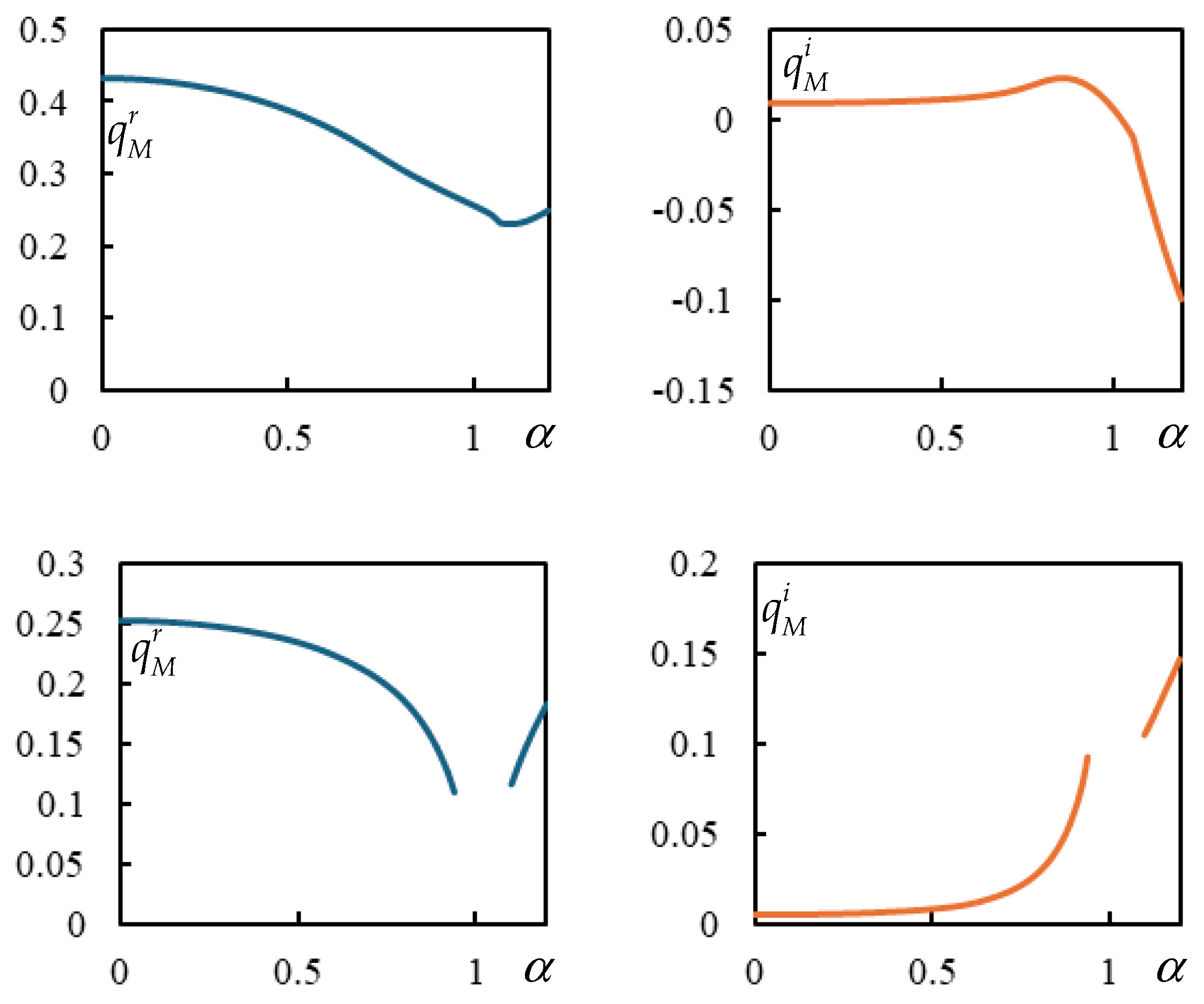
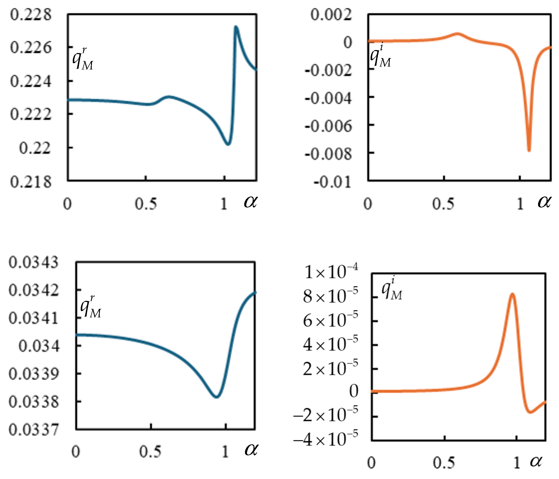
3.1. Induced Frequencies

To apply the closed-form formulas derived in Section 2, it is necessary to determine the complex roots of the characteristic equation:

$$E_{chr}=0$$

(48)

These roots are referred to as induced frequencies. As established in the author’s previous works, these frequencies can be efficiently determined using iterative procedures described therein. Generally, there are four pairs of roots, and as explained earlier, instability arises if at least one of these pairs is unstable.

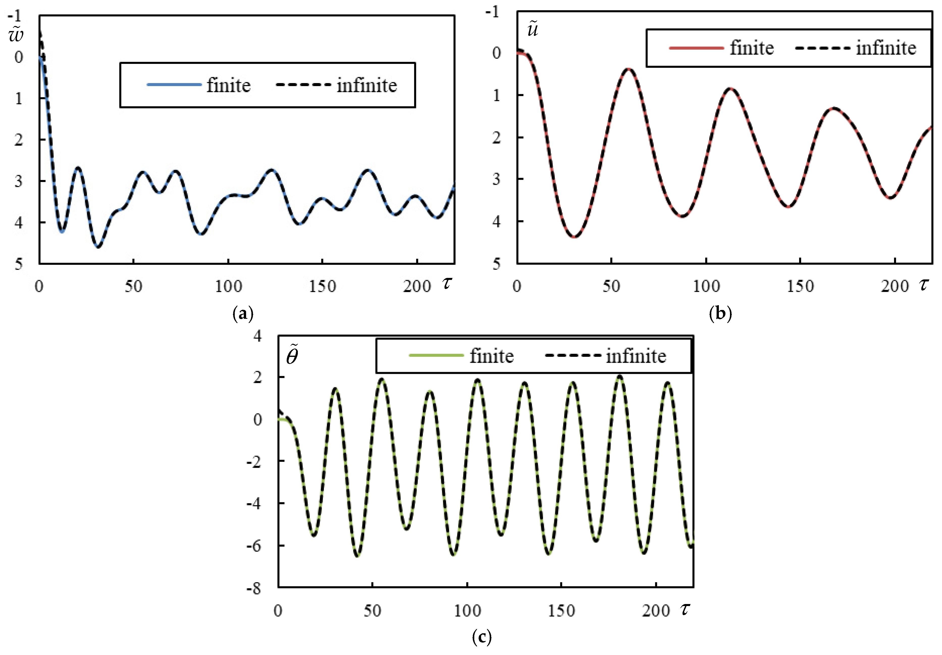
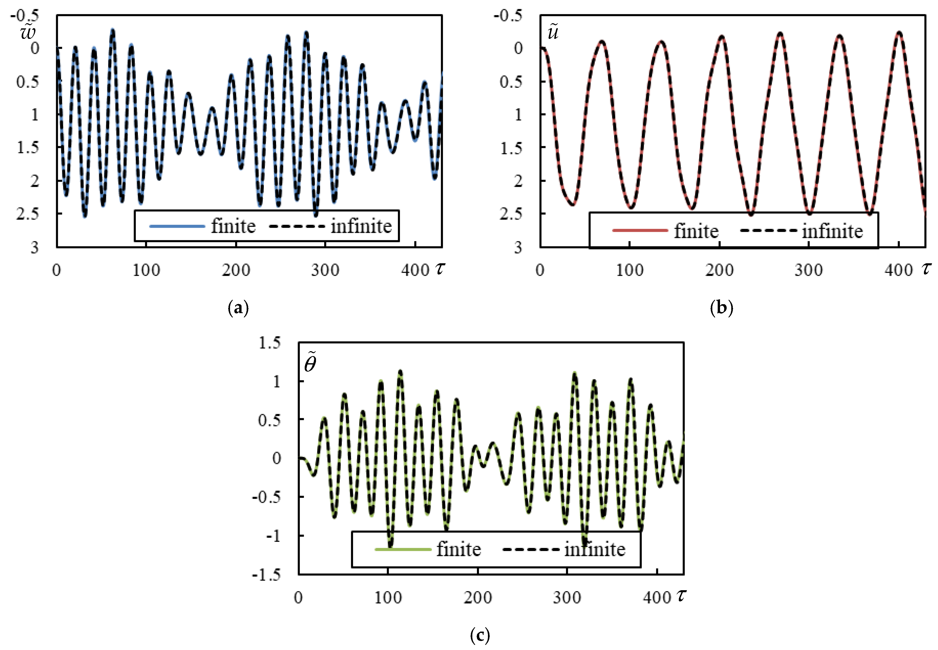
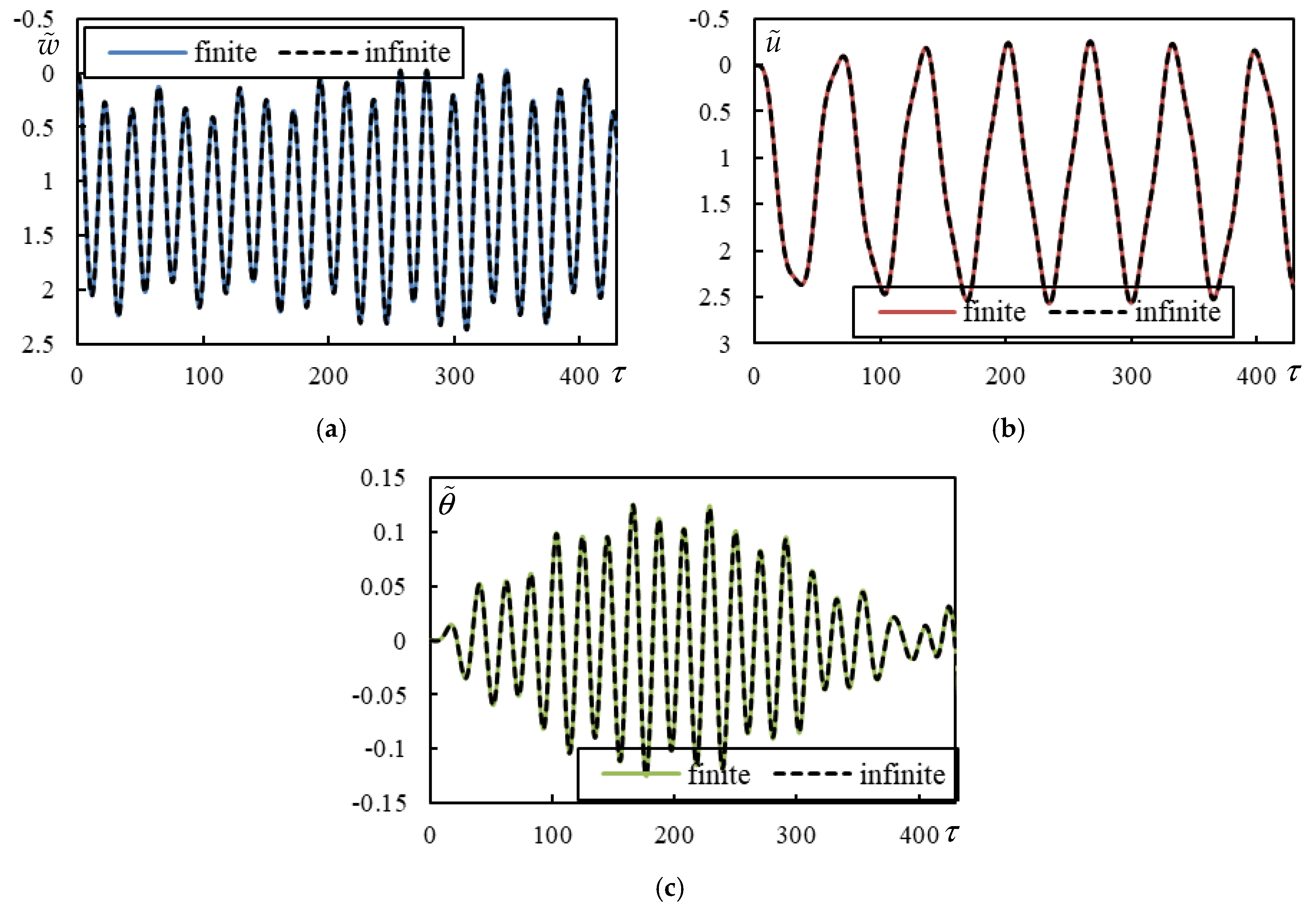
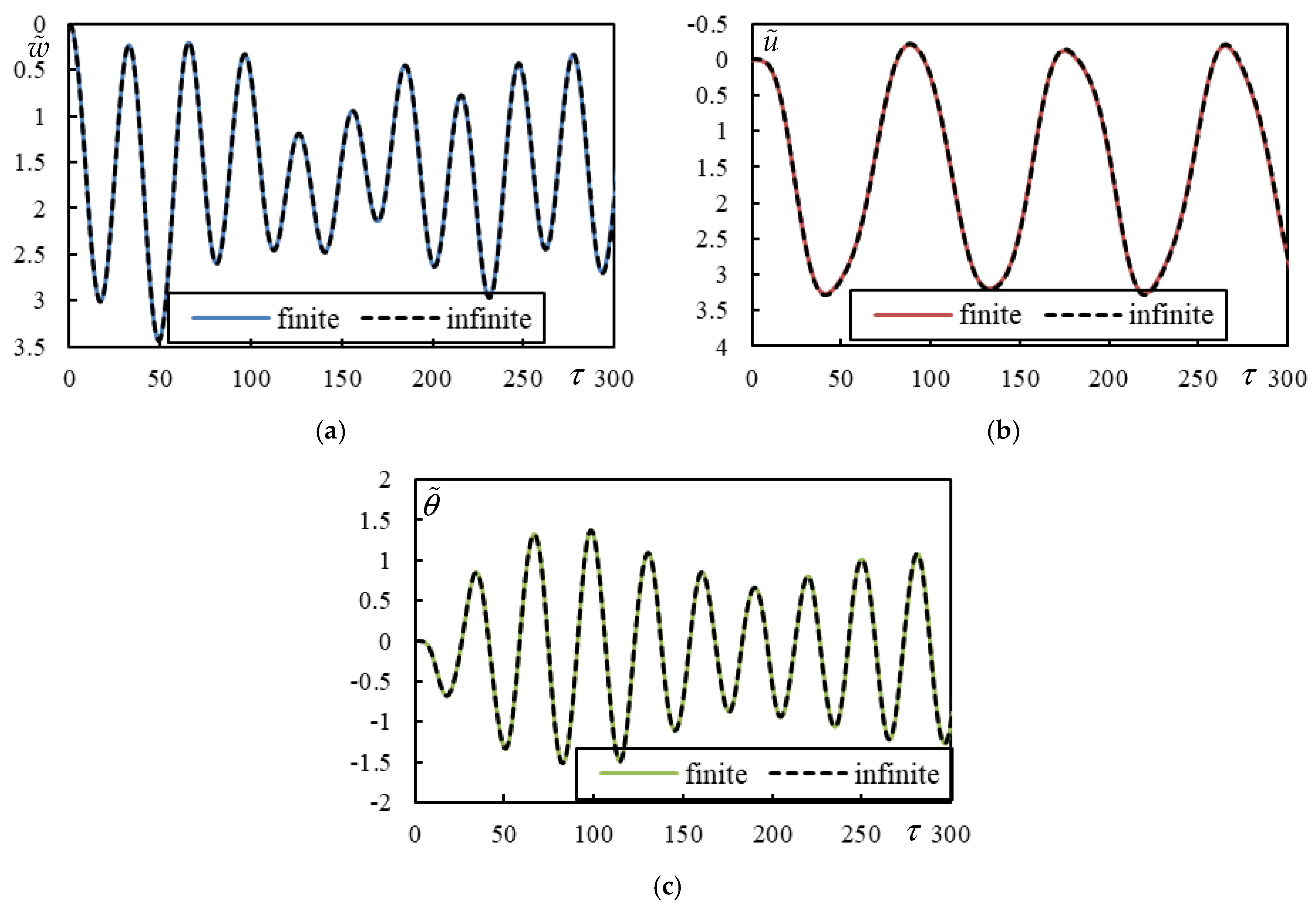
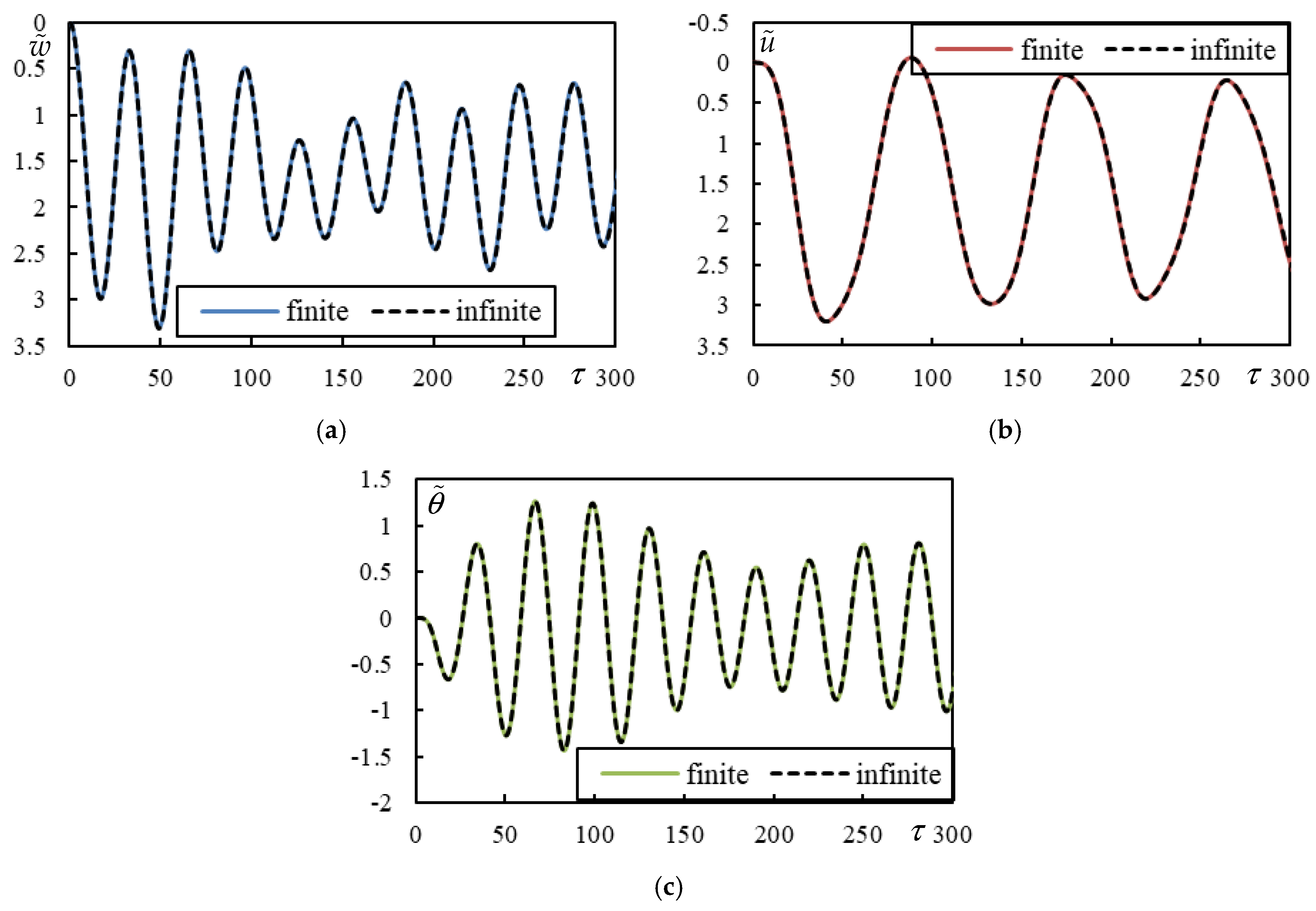
3.2. Validation on Finite Beams

Similar to previous studies, validation is performed on long finite beams using modal expansion. Given that the number of modes must be substantial, 500 modes were implemented in all tested cases to ensure accuracy while optimizing computational efficiency. It was confirmed that 500 modes were sufficient for all tested scenarios.

To solve the problem, the governing equations are retained in their original parameters and converted to dimensionless form only for comparison purposes. As in prior studies, without loss of generality, the beam is considered simply supported, as its vibration modes can then be expressed as sine functions, with modal frequencies and numbers determined analytically. In accordance with previous works, the loading is applied slightly off the left support to minimize its influence.

The beam equilibrium equations (Equations (1) and (7)) are multiplied by a mode shape and integrated over the beam length. In Equations (8) and (9), only the modal expansion of the beam deflection is introduced, after which all equations are assembled into a matrix form:

$$M\left(t\right)\cdot q_{,tt}\left(t\right)+C\left(t\right)\cdot q_{,t}\left(t\right)+K\left(t\right)\cdot q\left(t\right)=p\left(t\right)$$

(49)

The key step involves introducing additional variables:

$$\begin{array}{l}{Q}_{1,tt}=P-{\displaystyle \sum _{k}M{w}_k\left(vt\right)q_{k,tt}}-{\displaystyle \sum _k\left(2Mv{w}_{k,x}\left(vt\right)+c_v{w}_k\left(vt\right)\right)}{q}_{k,t}\\ -{\displaystyle \sum _k\left(M{v}^2{w}_{k,xx}\left(vt\right)+c_{v}v{w}_{k,x}\left(vt\right)+k_v{w}_k\left(vt\right)\right)}{q}_k\end{array}$$

(50)

$$\begin{array}{l}{Q}_{2,tt}=P-{\displaystyle \sum _{k}M{w}_k\left(vt+d\right)q_{k,tt}}-{\displaystyle \sum _k\left(2Mv{w}_{k,x}\left(vt+d\right)+c_v{w}_k\left(vt+d\right)\right)}{q}_{k,t}\\ -{\displaystyle \sum _k\left(M{v}^2{w}_{k,xx}\left(vt+d\right)+c_{v}v{w}_{k,x}\left(vt+d\right)+k_v{w}_k\left(vt+d\right)\right)}{q}_k\end{array}$$

(51)

resulting in the governing matrices for mass $M\left(t\right)$, damping $C\left(t\right)$, and stiffness $K\left(t\right)$ with the vector of unknowns $q\left(t\right)={\left[q_1,\dots q_n,u_v,\theta ,Q_1,Q_2\right]}^T$ and of the loading term $p\left(t\right)={\left[0,\dots 0,0,0,P,P\right]}^T$.

$$M\left(t\right)=\left[\begin{array}{ccccc}{\delta }_{jk}& 0& 0& -w_j\left(vt\right)& -w_j\left(vt+d\right)\\ 0& M_b& 0& 0& 0\\ 0& 0& J_b& 0& 0\\ M{w}_k\left(vt\right)& 0& 0& 1& 0\\ M{w}_k\left(vt+d\right)& 0& 0& 0& 1\end{array}\right]$$

(52)

$$C\left(t\right)=\left[\begin{array}{ccccc}{\delta }_{jk}{\displaystyle \frac{c_b}{m}}& -c_v{w}_j\left(vt\right)-c_v{w}_j\left(vt+d\right)& {\displaystyle \frac{1}{2}}d{c}_v{w}_j\left(vt\right)-{\displaystyle \frac{1}{2}}d{c}_v{w}_j\left(vt+d\right)& 0& 0\\ -c_v{w}_k\left(vt\right)-c_v{w}_k\left(vt+d\right)& 2c_v& 0& 0& 0\\ {\displaystyle \frac{d}{2}}\left(c_v{w}_k\left(vt\right)-c_v{w}_k\left(vt+d\right)\right)& 0& {\displaystyle \frac{1}{2}}{c}_v{d}^2& 0& 0\\ 2Mv{w}_{k,x}\left(vt\right)+c_v{w}_k\left(vt\right)& 0& 0& 0& 0\\ 2Mv{w}_{k,x}\left(vt+d\right)+c_v{w}_k\left(vt+d\right)& 0& 0& 0& 0\end{array}\right]$$

(53)

$$K\left(t\right)=\left[\begin{array}{ccccc}{\delta }_{jk}{\omega }_j^2& -k_v{w}_j\left(vt\right)-k_v{w}_j\left(vt+d\right)& {\displaystyle \frac{d}{2}}{k}_v{w}_j\left(vt\right)-{\displaystyle \frac{d}{2}}{k}_v{w}_j\left(vt+d\right)& 0& 0\\ \begin{array}{l}-k_v\left(w_k\left(vt\right)+w_k\left(vt+d\right)\right)\\ -c_{v}v\left(w_{k,x}\left(vt\right)+w_{k,x}\left(vt+d\right)\right)\end{array}& 2k_v& 0& 0& 0\\ \begin{array}{l}{\displaystyle \frac{d}{2}}{k}_v\left(w_k\left(vt\right)-w_k\left(vt+d\right)\right)\\ +{\displaystyle \frac{d}{2}}{c}_{v}v\left(w_{k,x}\left(vt\right)-w_{k,x}\left(vt+d\right)\right)\end{array}& 0& {\displaystyle \frac{1}{2}}{k}_v{d}^2& 0& 0\\ M{v}^2{w}_{k,xx}\left(vt\right)+k_v{w}_k\left(vt\right)+c_{v}v{w}_{k,x}\left(vt\right)& 0& 0& 0& 0\\ \begin{array}{l}+M{v}^2{w}_{k,xx}\left(vt+d\right)+k_v{w}_k\left(vt+d\right)\\ +c_{v}v{w}_{k,x}\left(vt+d\right)\end{array}& 0& 0& 0& 0\end{array}\right]$$

(54)

3.3. Timoshenko-Rayleigh Beam

When a Timoshenko beam is considered, Equation (1) is replaced by a set of equations:

$$-G\overline{A}{w}_{,xx}+G\overline{A}{\phi }_{,x}+m{w}_{,tt}+c_f{w}_{,t}+k_{f}w=\hspace{0.33em}p\left(x,t\right)$$

(55)

$$-G\overline{A}{w}_{,x}+G\overline{A}\phi +J{\phi }_{,tt}-EI{\phi }_{,xx}=\hspace{0.33em}0$$

(56)

where $G$ is the shear modulus, $\overline{A}$ is the reduced cross-sectional area, $\phi$ is the cross-sectional rotation angle and $J$ is the mass moment of inertia of the cross-section, which can be rewritten as $m{r}^2$ with $r$ being the radius of gyration.

By transitioning to moving coordinates, the equations transform into:

$$-G\overline{A}{w}_{,rr}+G\overline{A}{\phi }_{,r}+m\left(w_{,tt}-2v{w}_{,rt}+v^2{w}_{,rr}\right)+c_f\left(w_{,t}-v{w}_{,r}\right)+k_{f}w=p\left(r,t\right)$$

(57)

$$-G\overline{A}{w}_{,r}+G\overline{A}\phi +m{r}^2\left({\phi }_{,tt}-2v{\phi }_{,rt}+v^2{\phi }_{,rr}\right)-EI{\phi }_{,rr}=\hspace{0.33em}0$$

(58)

The introduction of additional dimensionless parameters:

$$\tilde{\phi }={\displaystyle \frac{\phi }{w_{st}\chi }}, \tilde{S}={\displaystyle \frac{G\overline{A}}{2\sqrt{k_{f}EI}}}, \tilde{r}=r\chi$$

(59)

further simplifies the problem, leading to:

$$-4\tilde{S}{\tilde{w}}_{,\xi \xi }+4\tilde{S}{\tilde{\phi }}_{,\xi }+4{\alpha }^2{\tilde{w}}_{,\xi \xi }+4{\tilde{w}}_{,\tau \tau }-8\alpha {\tilde{w}}_{,\xi \tau }+8{\eta }_f\left({\tilde{w}}_{,\tau }-\alpha {\tilde{w}}_{,\xi }\right)+4\tilde{w}=\tilde{p}\left(\xi ,\tau \right)$$

(60)

$$-4\tilde{S}{\tilde{w}}_{,\xi }+4\tilde{S}\tilde{\phi }+4{\tilde{r}}^2\left({\alpha }^2{\tilde{\phi }}_{,\xi \xi }-2\alpha {\tilde{\phi }}_{,\xi \tau }+{\tilde{\phi }}_{,\tau \tau }\right)-{\tilde{\phi }}_{,\xi \xi }=\hspace{0.33em}0$$

(61)

Applying integral transforms allows the solution of $\tilde{\phi }$:

$$\tilde{\Phi }=\hspace{0.33em}{\displaystyle \frac{4\mathrm{i}p\tilde{S}}{4\tilde{S}-4{\tilde{r}}^2{\left(\alpha p-q\right)}^2+p^2}}\tilde{W}$$

(62)

which is then substituted into the first equation. The subsequent steps follow the same derivation process as before.

3.4. Tested Cases

Multiple cases were analyzed to meet the objectives of this study. To define an admissible range of parameters, a broad spectrum of real-world values was considered. For the supporting structure, the parameters $EI$ and $m$ fall within a relatively narrow interval, approximately $EI\in 〈4.7;6.4〉{\mathrm{MNm}}^2$ and $m\in 〈54;60〉\mathrm{kg}/\mathrm{m}$, respectively. The parameter $k_s$ is sometimes omitted in similar models, allowing for a zero value, while variations are primarily assigned to $k_f\in 〈0.22;1000〉{\mathrm{MN}/\mathrm{m}}^2$.

Regarding the moving bogie, combining all possible parameter values would be impractical, as the bogie bar’s mass should relate to the wheel masses and, along with the wheel spacing, determine its mass moment of inertia. To account for this, two additional coefficients, $c{f}_1$ and $c{f}_2$, are introduced to link these values:

$${\mu }_v=c{f}_1{\eta }_M, {\tilde{J}}_b=c{f}_2{\eta }_M{\tilde{d}}^2$$

(63)

Using Equations (16) and (17), this also implies that:

$$M_b=c{f}_{1}M, J_b=c{f}_{2}M{d}^2$$

(64)

The primary suspension stiffness spans a wide range of values, and two representative values were selected: 0.02 for a soft suspension and 0.2 for a stiffer suspension. The damping parameters ${\eta }_f$ and ${\eta }_v$, as well as the velocity ratio $\alpha$, vary based on the effects being analyzed.

Table 1. Input data of cases analyzed in time series.

Parameter	${\mathit{\eta }}_{\mathit{f}}$	${\mathit{\eta }}_{\mathit{M}}$	$\tilde{\mathit{d}}$	$\mathit{c}{\mathit{f}}_{\mathbf{1}}$	$\mathit{c}{\mathit{f}}_{\mathbf{2}}$	${\mathit{\kappa }}_{\mathit{v}}$	${\mathit{\eta }}_{\mathit{v}}$	$\mathit{\alpha }$
Case 1	0.1	20	1	1.7	0.01	0.02	0	0.8
Case 2	0	20	2	2	0.1	0.2	0	0.5
Case 3	0	20	5	2	0.1	0.2	0	0.5
Case 4	0	20	5	1.7	0.1	0.2	0	0.5
Case 5	0.05	40	1.5	1.7	0.01	0.2	0	0.7
Case 6	0.05	40	1.5	1.7	0.01	0.2	0.05	0.7
Case 7	0.05	30	2	1.7	0.01	0.2	0.05	0.4
Case 8	0.05	30	2	1.7	0.01	0.2	0	0.4
Case 9	0	30	2	1.7	0.01	0.2	0.05	0.4
Case 10	0	30	2	1.7	0.01	0.2	0	0.4
Case 11	0.05	25	2	1.7	0.01	0.2	0.05	0.4
Case 12	0.15	50	1.5	1.7	0.1	0.2	0	0.85
Case 13	0.15	15	1	1.7	0.1	0.2	0	0.95

presents the input data for all tested cases, while

Table 2. Induced frequencies of analyzed cases.

Parameter	${\mathit{q}}_{{\mathit{M}}_{\mathbf{1}}}^{\mathit{r}}$	${\mathit{q}}_{{\mathit{M}}_{\mathbf{1}}}^{\mathit{i}}$	${\mathit{q}}_{{\mathit{M}}_{\mathbf{2}}}^{\mathit{r}}$	${\mathit{q}}_{{\mathit{M}}_{\mathbf{2}}}^{\mathit{i}}$	${\mathit{q}}_{{\mathit{M}}_{\mathbf{3}}}^{\mathit{r}}$	${\mathit{q}}_{{\mathit{M}}_{\mathbf{3}}}^{\mathit{i}}$	${\mathit{q}}_{{\mathit{M}}_{\mathbf{4}}}^{\mathit{r}}$	${\mathit{q}}_{{\mathit{M}}_{\mathbf{4}}}^{\mathit{i}}$
Case 1	±0.307227	0.021025	±0.222538	−0.000130	±0.184817	0.028535	±0.033910	0.000014
Case 2	±0.319059	0	±0.290698	0	±0.200435	0	±0.094072	0
Case 3	±0.310632	0	±0.294334	0	±0.200910	0	±0.094035	0
Case 4	±0.310639	0	±0.294718	0	±0.200910	0	±0.101860	0
Case 5	±0.505305	0.000454	±0.206528	−0.000472	±0.174711	0.007546	±0.070460	0.000121
Case 6	±0.501188	0.063327	±0.206521	0.000448	±0.174683	0.008301	±0.070451	0.001137
Case 7	±0.577601	0.084896	±0.255723	0.003197	±0.236572	0.004611	±0.083388	0.001565
Case 8	±0.583823	0.000110	±0.255859	0.001562	±0.236478	0.004163	±0.083397	0.000047
Case 9	±0.577617	0.084792	±0.255809	0.001646	±0.236376	0.000436	±0.083390	0.001518
Case 10	±0.583817	0	±0.255864	0	±0.236346	0	±0.083394	0
Case 11	±0.631225	0.101825	±0.279230	0.003868	±0.257027	0.005435	±0.091336	0.001877
Case 12	±0.186008	−0.000482	±0.148407	0.016963	±0.122981	0.013168	±0.062675	0.000636
Case 13	±0.354144	0.025958	±0.249576	−0.000631	±0.167778	0.148504	±0.113114	0.004749

summarizes the induced frequencies used in the residue evaluation.

The selection of cases shown in the time series, as well as the parameters listed in Table 1, was made as follows. Case 1 was selected as the only instance where the moving bogie performs worse than moving masses. Cases 2 and 3 were chosen to demonstrate that the strong dynamic interaction discussed in [56] for two moving masses is also present in the case of a moving bogie. Case 4 was selected for comparison with Case 3 to examine the effect of $c{f}_1$. Cases 2–4 are undamped, therefore, all amplitudes remain unchanged, the induced frequencies are real (Table 2), and these cases also serve to illustrate how undamped cases can be handled without numerical difficulties. Cases 5 and 6 were chosen such that Case 5 is unstable for subcritical velocity, but by adding damping to the primary suspension while keeping the other parameters unchanged, stability is achieved, leading to Case 6. Cases 7–10 demonstrate the effect of damping at different levels. A low damping level of 5% was chosen, and all four combinations were tested by applying damping to the foundation and/or primary suspension. Case 11 complements Case 7, highlighting the effect of changing the moving masses (wheels) value. The final two cases, Case 12 and Case 13, were selected to demonstrate instability in the subcritical velocity range, however, unlike Cases 1 or 5, instability arises here even for a higher mass moment of inertia of the bogie bar.

The general trend of the frequency lines is illustrated in Figure 2, using the parameters of Case 1 but extending over the entire velocity range. Since the values are significantly different, they are plotted separately. In general, four pairs of induced frequencies can be observed. Their evolution is interrupted when their imaginary part reaches ${\eta }_f$, as demonstrated in [40].

Unlike more complex models, the critical velocity for resonance in this study is well-defined by an analytical formula, referring to the critical velocity of a single constant force moving at a constant velocity over the one-layer model:

$${\alpha }_{cr}^{E-B}={\alpha }_{ref}\sqrt{1+{\eta }_s} \mathrm{with} {\alpha }_{ref}=1$$

(65)

For the Timoshenko-Rayleigh beam, the critical velocity is presented, for instance, in [71] or [67]. Expressed in the dimensionless parameters used here, it becomes more explicit how this value relates to that of the Euler-Bernoulli beam:

$${\alpha }_{cr}^{T-R}={\alpha }_{ref}{\displaystyle \frac{\sqrt{{\tilde{r}}^2-\tilde{S}-8{\tilde{r}}^2{\tilde{S}}^2+4{\tilde{S}}^{3/2}\sqrt{4{\tilde{r}}^4\tilde{S}-{\tilde{r}}^2+\tilde{S}}}}{2\left(\tilde{S}-{\tilde{r}}^2\right)}} \mathrm{with} {\alpha }_{ref}=1$$

(66)

3.5. Comparison with Moving Masses

Unlike a single moving inertial object with a single contact point on the supporting structure, which cannot experience instability in the subcritical velocity range, multiple moving objects can interact dynamically, leading to subcritical instability. Instability at subcritical velocity is common but, in many cases, requires unrealistically high mass values, as shown in [56].

To summarize the negative effects of foundation damping, Figure 3 illustrates the instability lines for different levels of damping. To illustrate the analyzed features and provide insight into general tendencies, the vertical axis is extended up to ${\eta }_M=200$, which is already an academic value. The parameter $\alpha$ extends up to 1.2, where $\alpha =1$ corresponds to the critical velocity for resonance. For simplicity and to maintain consistency with the moving bogie case, two equal moving masses subjected to the same constant forces are considered. In dimensionless parameters, when the effect of shear stiffness is neglected, the only variables are the distance between the masses and foundation damping.

The instability lines were traced by identifying real-valued induced frequencies, which in damped cases necessarily alter the number of unstable frequencies by one. This method clearly delineates stable and unstable velocity intervals for specific moving mass ratios and is both more effective and simpler than the traditional D-decomposition method used by other researchers (e.g., [67,68,69]).

Figure 3 demonstrates that increasing damping shifts all instability branches to lower moving masses while also making them straighter. Consequently, lower masses occupy larger velocity intervals, proving that, contrary to expectations, foundation damping worsens instability. However, in closed intervals, the degree of instability is generally lower than in semi-closed intervals.

In Figure 3, only relevant distances between masses are included, specifically those that still contain part of the branch within the defined scale in the subcritical velocity range. A broader analysis of distances between masses reveals that the starting point of the first instability branch shifts leftward as the distance increases, while at the same time, the moving masses increase.

When considering the moving bogie, additional parameters come into play. To make the comparison more realistic, the total mass should remain the same. Figure 4 presents the case where $c{f}_1=1.7$, requiring the instability lines from Figure 3 to be recalculated accordingly, to be comparable. In addition to $c{f}_1=1.7$, the moving bogie is characterized by $c{f}_2=0.01$ and ${\kappa }_v=0.02$, chosen to minimize its influence as much as possible.

It can be concluded that even for weak primary suspension stiffness and a low mass moment of inertia of the bogie bar, all cases with a moving bogie perform better—meaning the instability lines are positioned above those for moving masses—except for the lowest tested distance $\tilde{d}=1$. The instability lines in Figure 4 are represented only up to the critical velocity. The relevant instability lines are those that contain a segment within the chosen scale in the subcritical velocity range. The following rule applies: if a particular instability line ($\tilde{d}$) is relevant for moving masses but not for a moving bogie, then $\tilde{d}+0.25$ is not plotted for moving masses, even if it would otherwise be considered relevant.

To analyze in detail the only case where the moving bogie performs worse than moving masses, Case 1 from Table 1 is selected. This case is unstable. However, as shown in Table 2, the unstable frequency has a relatively low imaginary part (in absolute value). This implies that the instability becomes significant only at later times, while initially, this case behaves similarly to a highly damped system. Figure 5 presents time series obtained using closed-form formulas, as well as results from a finite beam model for validation. The high-time behavior shown in Figure 6 is calculated exclusively using closed-form formulas, as performing these calculations on a finite beam would be computationally prohibitive due to the excessive number of vibration modes. Similarly, numerical integration would be impractical due to limitations in numerical precision.

3.6. Effect of Suspension Damping

Suspension damping has a significantly positive impact on bogie stability, an effect further enhanced by a higher mass moment of inertia of the bogie bar. To demonstrate this, $c{f}_1=1.7$, and the other coefficient varies between $c{f}_2=0.01$ and $c{f}_2=0.1$. A weak foundation damping of ${\eta }_f=0.05$ and a stiffer primary suspension stiffness of ${\kappa }_v=0.2$ are implemented.

Figure 7 clearly shows that, with a higher mass moment of inertia of the bogie bar, nearly all instability lines for the cases with primary suspension damping are removed from the subcritical velocity range.

3.7. Impact of Beam Theory on the Results

To assess the influence of beam theory on the results, two cases are analyzed in Figure 8. Since the additional parameters in the Timoshenko-Rayleigh theory must be chosen consistently, as is clear from Equation (59), the values for a softer foundation $\tilde{S}=100$ and $\tilde{r}=0.03$, and for a stronger foundation $\tilde{S}=10$ and $\tilde{r}=0.09$, were selected. The other parameters are: $c{f}_1=1.7$ and $c{f}_2=0.1$. Weak foundation damping of ${\eta }_f=0.05$ and a stiffer primary suspension stiffness of ${\kappa }_v=0.2$ with no damping are used.

Only the subcritical velocity range is shown. However, since the difference in critical velocity in the Timoshenko-Rayleigh case using Equation (66) is very small—0.993 and 0.980, respectively—the graphs are plotted up to the value of 1, as before.

The results indicate that for a softer foundation, there is virtually no difference between the Euler-Bernoulli and Timoshenko-Rayleigh theories. Some differences are noticeable for a stronger foundation, but they do not appear to be fundamental.

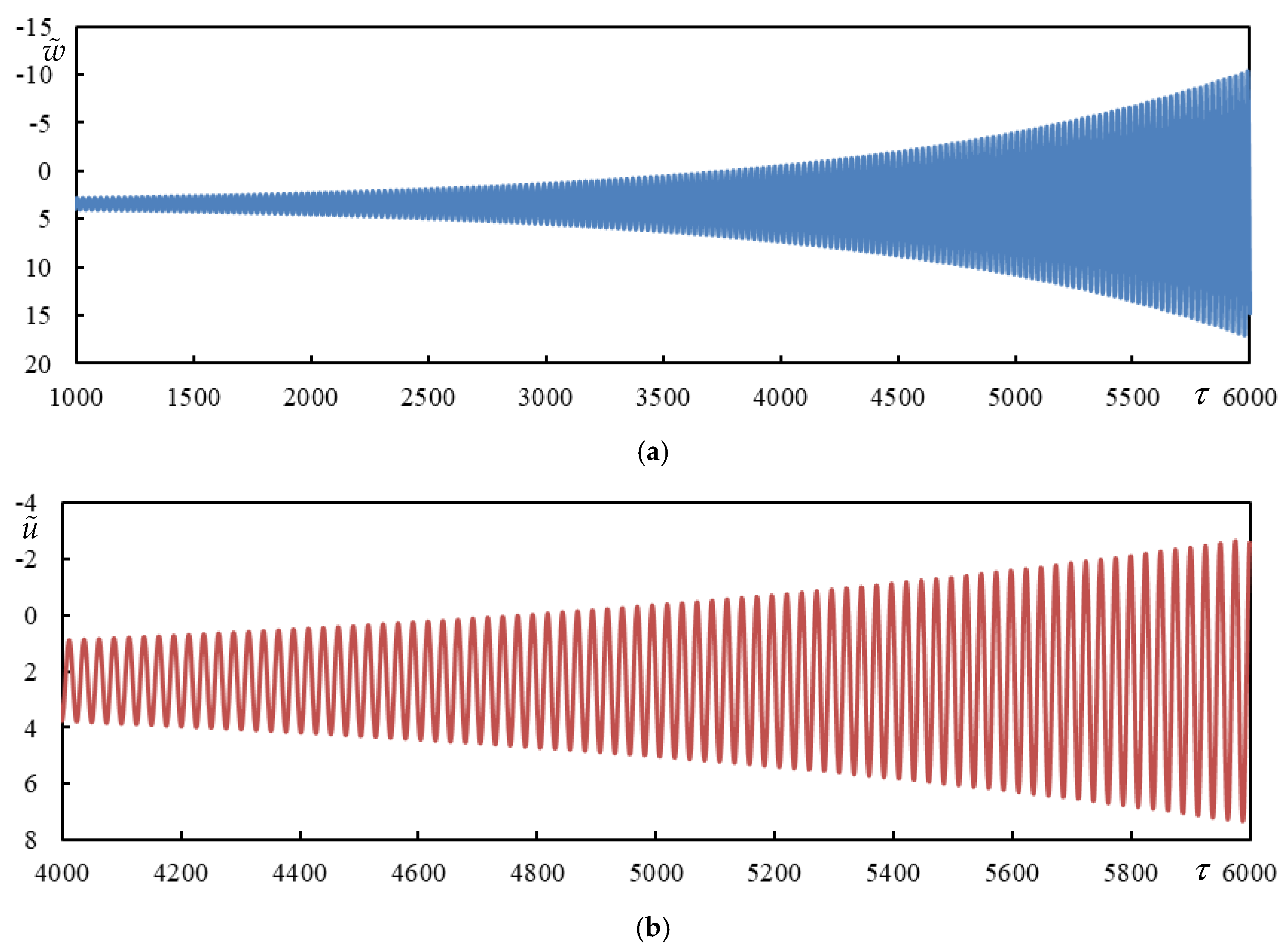
3.8. Time Series of Other Cases from Table 1

This subsection has three objectives: to analyze the effect under consideration, to demonstrate the ease of using closed-form formulas, and to verify that the contribution of integration along the branch cuts is negligible by comparing results with finite beam analysis.

Further time series analyses are conducted for Cases 2–6 from Table 1, comparing finite and infinite beam models. These cases explore dynamic interactions, stability effects, and induced frequency variations under different conditions. Cases 2 and 3 are selected to show that the dynamic interaction discussed in previous works for two moving masses is maintained for a moving bogie. A slightly higher parameter $c{f}_1=2$ is introduced, but the changes are not significant. Two distances are compared ($\tilde{d}=2$ in Figure 9 and $\tilde{d}=5$ in Figure 10). Other parameters are included in Table 1.

Figure 9 shows a strong dynamic interaction. In Figure 10, this effect is less pronounced, however, similar to the two moving masses case, dynamic interaction persists up to relatively high distances. Only when $K_{+}$ and $K_{-}$ start to have negligible values relative to $K_0$, then the interaction become negligible. This proves that the function envelopes for $\tilde{\theta }$ still show a very strong interaction in Figure 10 because $K_0$ is not included in Equation (43).

Case 4 is selected for comparison with Case 3 to assess the effect of $c{f}_1=1.7$ with respect to $c{f}_1=2$. In addition to the time series (Figure 11), differences in induced frequencies are also examined in Table 2.

Cases 2–4 are undamped, therefore, all amplitudes remain unchanged, and the induced frequencies are real (Table 2). These cases also serve to demonstrate that undamped cases can be handled without numerical problems.

Cases 5 and 6 are chosen such that Case 5 is unstable for subcritical velocity, but by adding damping to the primary suspension while keeping other parameters unchanged, it becomes stable (Case 6). Time series of Case 5 are shown in Figure 12. During the initial stages, there is no indication of instability as the rate of instability is very low (Table 2). The unstable frequency surpasses the stable ones only at higher times (Figure 13).

Case 6 is already stable. Times series are shown in Figure 14 for initial stages and in Figure 15 for higher times.

The other cases from Table 1 are summarized in Appendix A.

3.9. Comparison with Other Published Works

While [68] presents only isolated cases, Ref. [67] offers an evolution over a range of velocities, providing better insight into the problem. However, the reference case in [67] assumes a large distance between wheels (15 m), making it more of a simplified vehicle with two axles than an actual bogie. The evolution of the critical stiffness of the primary suspension is chosen for comparison. The results are shown in Figure 16 using the input data from [67].

It can be concluded that there is very good agreement after recalculating to dimensionless data as in [67]. Minor differences can be attributed to improvements in symbolic software, which now allow for higher accuracy and faster evaluation compared to when [67] was written.

In [67,68,69], the distance between wheels is so large that dynamic interaction is not significant, and as a result, instability in the subcritical velocity range does not occur.

4. Discussion

This paper presents a detailed analysis of the instability of a bogie passing through a one-layer model, focusing on the possibility that this may occur in the subcritical velocity range. All presented results were obtained (semi)analytically, quickly, and with very high accuracy.

The results of two moving proximate masses are used as a reference case, and it is shown that in general, the more realistic the moving object, the lower the risk of instability at such low velocities. This was confirmed even under the conditions of neglected suspension damping, reduced suspension stiffness, and small mass moment of inertia of the bogie bar. On the other hand, it was confirmed that the negative effect of foundation damping found in the two moving mass cases is preserved for the moving bogie. This effect is in contrast to the effect of foundation damping in the case of a single moving inertial object, where increased damping always shifts the onset of instability to higher velocities.

It has been demonstrated in selected examples that instability lines related to moving bogies have more branches than those related to moving masses, which complicates the analysis.

It has been shown in selected examples that suspension damping improves the unstable behavior in all cases, but it is much more efficient with a higher mass moment of inertia of the bogie bar.

As each of the presented examples covers a large range of possible scenarios due to its unidimensional nature, these conclusions might be considered general. Nevertheless, further studies are required as it would be exhaustive to explore the full admissible domain of all involved parameters.

Regarding the distances between the masses, it is not necessarily true that the lowest values indicate worse stability. Larger distances shift the starting point of the first instability branch to lower velocities, but at the same time, the smallest moving mass ratio of such a branch increases. Therefore, it is necessary to balance these two tendencies.

It has been proven that there are cases with realistic parameters where instability occurs in the subcritical velocity range. This article serves as a warning that instability at supercritical velocities cannot be taken for granted a priori. Nevertheless, it is necessary to bear in mind that the model, especially for the supporting structure, is very simple, and further research and validation are required.

Unlike all other works published by other researchers (e.g., [67,68,69]), where instability is determined by the D-decomposition method, here the so-called lines of instability are traced in the plane of velocity-moving mass ratios by identifying the real-valued induced frequencies. In a damped case, these frequencies necessarily alter the number of unstable induced frequencies by one, so that stable and unstable velocity intervals are clearly visible for any specific moving mass ratio. This approach is much more powerful and simpler than the D-decomposition method.

The presented analysis can be easily extended to other types of supporting structures since all expressions can be used for more complicated foundation models by simply replacing Equation (24) with an equation reflecting the new foundation model. There is only one complication: in other foundation models, the analytical formulas have limited use since discontinuities in the $K$-function prevent resolving all necessary induced frequencies for all velocities. This is only relevant for the time series—the instability lines are not affected. As an alternative for the time series, either numerical integration or finite models can be used.

5. Conclusions

In this paper, the possibility of instability in the subcritical range of velocities was discussed in detail. The results presented are easy to use, as the dimensionless parameters cover a wide range of possible scenarios, and the instability lines provide an overall view of the onset or aggravation of unstable behavior or the recovery of stable behavior. Such comprehensive information is very useful, as readers do not have to repeat the calculations and can use their dimensionless parameters for the case they are analyzing. However, it would be exhaustive to explore the full admissible domain of all involved parameters. Therefore, it would be incorrect to state that all possible cases are covered by the graphs presented in this paper.

The validation of the results on finite beams is clearly described and easily applicable to other researchers. The author of this paper believes that this is simpler than numerical integration associated with the inverse Laplace transform, which is numerically sensitive.

The unstable induced frequencies compared to the stable ones provide an initial estimate of the degree of instability. Indeed, it can be seen in Table 2 that the unstable frequencies of the selected cases have a relatively low imaginary part (in absolute value). As has been shown, the effect of foundation damping worsens instability. However, during the initial stages, it has a strong impact on the stable frequencies, making the vibrations initially resemble heavily damped cases. The unstable frequency only surpasses the stable ones at higher times. This is important for assessing the severity of instability and can be used in vibration mitigation measures. Since the analysis allows for the determination of vibration amplitude, together with the degree of instability, it identifies the time required for the unstable harmonics to overcome the stable ones. For this reason, it is important to have analytical formulas that are not affected by numerical approximations during numerical integration so that the time response can be extended as needed.

The main limitation of the results presented in this paper is the simplicity of the supporting structure, modeled as a one-layer system. It is well known that the one-layer model significantly overestimates the critical velocity of the railway track. In light of this, the results should be understood in a qualitative manner, as the ratio of the train’s velocity to the critical velocity is important, rather than the absolute values of these quantities. In order to make more general conclusions, it is necessary to extend the model to at least a three-layer system and include nonlinear behavior. The method is easily extendable to other layered models, and the nonlinearity is planned to be incorporated using Adomian decomposition. This will be the subject of further research.

References

1. Rodrigues, A.S.F.; Dimitrovová, Z. Applicability of a three-layer model for the dynamic analysis of ballasted railway tracks. Vibration 2021, 4, 151–174. [Google Scholar] [CrossRef]
2. Dimitrovová, Z. On the critical velocity of moving force and instability of moving mass in layered railway track models by semianalytical approaches. Vibration 2023, 6, 113–146. [Google Scholar] [CrossRef]
3. Grassie, S.L.; Gregory, R.W.; Harrison, D.; Johnson, K.L. The dynamic response of railway track to high frequency vertical excitation. J. Mech. Eng. Sci. 1982, 24, 77–90. [Google Scholar] [CrossRef]
4. Knothe, K.L.; Grassie, S.L. Modelling of railway track and vehicle-track interaction at high frequencies. Veh. Syst. Dyn. 1993, 22, 209–262. [Google Scholar] [CrossRef]
5. Dahlberg, T. Vertical dynamic train/track interaction—Verifying a theoretical model by full-scale experiments. Veh. Syst. Dyn. 1995, 24, 45–57. [Google Scholar] [CrossRef]
6. Zhai, W.; Cai, Z. Dynamic interaction between a lumped mass vehicle and a discretely supported continuous rail track. Comput. Struct. 1997, 63, 987–997. [Google Scholar] [CrossRef]
7. Oscarsson, J.; Dahlberg, T. Dynamic train/track/ballast interaction—Computer models and full-scale experiments. Veh. Syst. Dyn. 1998, 29, 73–84. [Google Scholar] [CrossRef]
8. Oscarsson, J. Dynamic train-track interaction: Variability attributable to scatter in the track properties. Veh. Syst. Dyn. 2002, 37, 59–79. [Google Scholar] [CrossRef]
9. Oscarsson, J. Simulation of train-track interaction with stochastic track properties. Veh. Syst. Dyn. 2002, 37, 449–469. [Google Scholar] [CrossRef]
10. Bureika, G.; Subačius, R. Mathematical model of dynamic interaction between wheel-set and rail track. Transport 2002, 17, 46–51. [Google Scholar] [CrossRef]
11. Lei, X.; Noda, N.A. Analyses of dynamic response of vehicle and track coupling system with random irregularity of track vertical profile. J. Sound Vib. 2002, 258, 147–165. [Google Scholar] [CrossRef]
12. Kouroussis, G.; Gazetas, G.; Anastasopoulos, I.; Conti, C.; Verlinden, O. Discrete modelling of vertical track-soil coupling for vehicle-track dynamics. Soil Dyn. Earthq. Eng. 2011, 31, 1711–1723. [Google Scholar] [CrossRef]
13. Nguyen, K.; Goicolea, J.M.; Galbadon, F. Comparison of dynamic effects of high-speed traffic load on ballasted track using a simplified two-dimensional and full three-dimensional model. Proc. Inst. Mech. Eng. Part F J. Rail Rapid Transit 2014, 228, 128–142. [Google Scholar] [CrossRef]
14. Zhai, M.W.; Wang, K.Y.; Lin, J.H. Modelling and experiment of railway ballast vibrations. J. Sound Vib. 2004, 270, 673–683. [Google Scholar] [CrossRef]
15. Ahlbeck, D.R.; Meacham, H.C.; Prause, R.H. The development of analytical models for railroad track dynamics. In Railroad Track Mechanics and Technology; Pergamon Press: Oxford, UK, 1975. [Google Scholar] [CrossRef]
16. Doyle, N.F. Railway Track Design: A Review of Current Practice. Bureau of Transport Economics (BTE), 1980. Available online: https://www.bitre.gov.au/sites/default/files/op_035.pdf (accessed on 13 March 2025).
17. Kerr, D. On the determination of the rail support modulus k. Int. J. Solids Struct. 2000, 37, 4335–4351. [Google Scholar] [CrossRef]
18. Zhai, W.M.; Sun, X. A detailed model for investigating vertical interaction between railway vehicle and track. Veh. Syst. Dyn. 1994, 23, 603–615. [Google Scholar] [CrossRef]
19. Beskou, N.D.; Muho, E.V. Review on dynamic response of road pavements to moving vehicle loads; part 1: Rigid pavements. Soil. Dyn. Earthq. Eng. 2023, 175, 108249. [Google Scholar] [CrossRef]
20. Muho, E.V.; Beskou, N.D. Review on dynamic analysis of road pavements under moving vehicles and plane strain conditions. J. Road Eng. 2024, 4, 54–68. [Google Scholar] [CrossRef]
21. Dimitrovová, Z. Semi-analytical analysis of vibrations induced by a mass traversing a beam supported by a finite depth foundation with simplified shear resistance. Meccanica 2020, 55, 2353–2389. [Google Scholar] [CrossRef]
22. Ouyang, L.; Xiang, Z.; Zhen, B.; Yuan, W. Analytical Study on the Impact of Nonlinear Foundation Stiffness on Pavement Dynamic Response under Vehicle Action. Appl. Sci. 2024, 14, 8705. [Google Scholar] [CrossRef]
23. Hua, X.; Zatar, W.; Cheng, X.; Chen, G.S.; She, Y.; Xu, X.; Liao, Z. Modeling and Characterization of Complex Dynamical Properties of Railway Ballast. Appl. Sci. 2024, 14, 11224. [Google Scholar] [CrossRef]
24. Yang, J.; He, X.; Jing, H.; Wang, H.; Tinmitonde, S. Dynamics of Double-Beam System with Various Symmetric Boundary Conditions Traversed by a Moving Force: Analytical Analyses. Appl. Sci. 2019, 9, 1218. [Google Scholar] [CrossRef]
25. Zhao, L.; Wang, S.-L. Analytical determination of critical velocity and frequencies of beam with moving mass under different supporting conditions. J. Vibroeng. 2024, 26, 1014–1026. [Google Scholar] [CrossRef]
26. Al-Ashtari, W. A new approach for modelling the vibration of beams under moving load effect. ARPN J. Eng. Appl. Sci. 2023, 18, 1195–1206. [Google Scholar]
27. Ghannadiasl, A.; Mofid, M. Sensitivity analysis of vibration response of timoshenko beam to mass ratio and velocity of moving mass and boundary conditions: Semi-analytical approach. Forces Mech. 2023, 11, 100205. [Google Scholar] [CrossRef]
28. Zhou, R.; Yang, P.; Li, Y.; Tao, Y.G.; Xu, J.; Zhu, Z. Interfacial properties of double-block ballastless track under various environmental conditions. Int. J. Mech. Sci. 2024, 266, 108954. [Google Scholar] [CrossRef]
29. Dumitriu, M. Fault detection of damper in railway vehicle suspension based on the cross-correlation analysis of bogie accelerations. Mech. Ind. 2019, 20, 102. [Google Scholar] [CrossRef]
30. Heydari, H. Evaluating the dynamic behavior of railway-bridge transition zone: Numerical and field measurements. Can. J. Civil Eng. 2024, 51, 399–408. [Google Scholar] [CrossRef]
31. Jain, A.; Metrikine, A.V.; Steenbergen, M.J.M.M.; van Dalen, K.N. Railway Transition Zones: Energy Evaluation of a Novel Transition Structure for Critical Loading Conditions. J. Vib. Eng. Technol. 2025, 13, 15. [Google Scholar] [CrossRef]
32. Uranjek, M.; Imamović, D.; Peruš, I. Mathematical Modeling of the Floating Sleeper Phenomenon Supported by Field Measurements. Mathematics 2024, 12, 3142. [Google Scholar] [CrossRef]
33. Li, Z.; Li, S.; Zhang, P.; Núñez, A.; Dollevoet, R. Mechanism of short pitch rail corrugation: Initial excitation and frequency selection for consistent initiation and growth. Int. J. Rail Transp. 2024, 12, 13150. [Google Scholar] [CrossRef]
34. Zhang, P.; He, C.; Shen, C.; Dollevoet, R.; Li, Z. Comprehensive validation of three-dimensional finite element modelling of wheel-rail high-frequency interaction via the V-Track test rig. Veh. Syst. Dyn. 2024, 62, 2785–2809. [Google Scholar] [CrossRef]
35. Fărăgău, A.B.; Metrikine, A.V.; van Dalen, K.N. Transition radiation in a piecewise-linear and infinite one-dimensional structure–a Laplace transform method. Nonlinear Dyn. 2019, 98, 2435–2461. [Google Scholar] [CrossRef]
36. Fărăgău, A.B.; Keijdener, C.; de Oliveira Barbosa, J.M.; Metrikine, A.V.; van Dalen, K.N. Transition radiation in a nonlinear and infinite one-dimensional structure: A comparison of solution methods. Nonlinear Dyn. 2021, 103, 1365–1391. [Google Scholar] [CrossRef]
37. Fărăgău, A.B.; Mazilu, T.; Metrikine, A.V.; Tao, L.; van Dalen, K.N. Transition radiation in an infinite one-dimensional structure interacting with a moving oscillator—The Green’s function method. J. Sound Vib. 2021, 492, 115804. [Google Scholar] [CrossRef]
38. Gao, L.; Shi, S.; Zhong, Y.; Xu, M.; Xiao, Y. Real-time evaluation of mechanical qualities of ballast bed in railway tamping maintenance. Int. J. Mech. Sci. 2023, 248, 108192. [Google Scholar] [CrossRef]
39. Yang, Y.B.; Gao, S.Y.; Shi, K.; Mo, X.Q.; Yuan, P.; Wang, H.Y. Selection of the Span Length of an Analogic Finite Beam to Simulate the Infinite Beam Resting on Viscoelastic Foundation Under a Harmonic Moving Load. Int. J. Struct. Stab. Dyn. 2025, 2540001. [Google Scholar] [CrossRef]
40. Dimitrovová, Z. Semi-analytical solution for a problem of a uniformly moving oscillator on an infinite beam on a two-parameter visco-elastic foundation. J. Sound Vib. 2019, 438, 257–290. [Google Scholar] [CrossRef]
41. Dimitrovová, Z. A General Procedure for the Dynamic Analysis of Finite and Infinite Beams on Piece-Wise Homogeneous Foundation under Moving Loads. J. Sound Vib. 2010, 329, 2635–2653. [Google Scholar] [CrossRef]
42. Dimitrovová, Z. Two-layer model of the railway track: Analysis of the critical velocity and instability of two moving proximate masses. Int. J. Mech. Sci. 2022, 217, 107042. [Google Scholar] [CrossRef]
43. Dimitrovová, Z. Complete semi-analytical solution for a uniformly moving mass on a beam on a two-parameter visco-elastic foundation with non-homogeneous initial conditions. Int. J. Mech. Sci. 2018, 144, 283–311. [Google Scholar] [CrossRef]
44. Zhang, S.; Fan, W.; Yang, C. Semi-analytical solution to the steady-state periodic dynamic response of an infinite beam carrying a moving vehicle. Int. J. Mech. Sci. 2022, 226, 107409. [Google Scholar] [CrossRef]
45. Mazilu, T.; Răcănel, I.R.; Gheți, M.A. Vertical interaction between a driving wheelset and track in the presence of the rolling surfaces harmonic irregularities. Rom. J. Transp. Infrastruct. 2020, 9, 38–52. [Google Scholar] [CrossRef]
46. Kiani, K.; Nikkhoo, A. On the limitations of linear beams for the problems of moving mass-beam interaction using a meshfree method. Acta Mech. Sin. 2011, 28, 164–179. [Google Scholar] [CrossRef]
47. Kiani, K.; Nikkhoo, A.; Mehri, B. Prediction capabilities of classical and shear deformable beam models excited by a moving mass. J. Sound Vib. 2009, 320, 632–648. [Google Scholar] [CrossRef]
48. Kiani, K.; Nikkhoo, A.; Mehri, B. Assessing dynamic response of multispan viscoelastic thin beams under a moving mass via generalized moving least square method. Acta Mech. Sin. 2010, 26, 721–733. [Google Scholar] [CrossRef]
49. Jahangiri, A.; Attari, N.K.A.; Nikkhoo, A.; Waezi, Z. Nonlinear dynamic response of an Euler–Bernoulli beam under a moving mass–spring with large oscillations. Arch. Appl. Mech. 2020, 90, 1135–1156. [Google Scholar] [CrossRef]
50. Tran, M.T.; Ang, K.K.; Luong, V.H. Vertical dynamic response of non-uniform motion of high-speed rails. J. Sound Vib. 2014, 333, 5427–5442. [Google Scholar] [CrossRef]
51. Dai, J.; Lim, J.G.Y.; Ang, K.K. Dynamic response analysis of high-speed maglev-guideway system. J. Vib. Eng. Technol. 2023, 11, 2647–2658. [Google Scholar] [CrossRef]
52. Stojanović, V.; Kozić, P.; Petković, M.D. Dynamic instability and critical velocity of a mass moving uniformly along a stabilized infinity beam. Int. J. Solids Struct. 2017, 108, 164–174. [Google Scholar] [CrossRef]
53. Dimitrovová, Z. New semi-analytical solution for a uniformly moving mass on a beam on a two-parameter visco-elastic foundation. Int. J. Mech. Sci. 2017, 127, 142–162. [Google Scholar] [CrossRef]
54. Metrikine, A.V.; Verichev, S.N.; Blaauwendraad, J. Stability of a two-mass oscillator moving on a beam supported by a visco-elastic half-space. Int. J. Solids Struct. 2005, 42, 1187–1207. [Google Scholar]
55. Mazilu, T.; Dumitriu, M.; Tudorache, C. Instability of an oscillator moving along a Timoshenko beam on viscoelastic foundation. Nonlinear Dyn. 2012, 67, 1273–1293. [Google Scholar] [CrossRef]
56. Dimitrovová, Z. Dynamic interaction and instability of two moving proximate masses on a beam on a Pasternak viscoelastic foundation. Appl. Math. Modell. 2021, 100, 192–217. [Google Scholar] [CrossRef]
57. Mazilu, T. Instability of a train of oscillators moving along a beam on a viscoelastic foundation. J. Sound Vib. 2013, 332, 4597–4619. [Google Scholar] [CrossRef]
58. Yang, B.; Gao, H.; Liu, S. Vibrations of a Multi-Span Beam Structure Carrying Many Moving Oscillators. Int. J. Struct. Stab. Dyn. 2018, 18, 1850125. [Google Scholar] [CrossRef]
59. Stojanović, V.; Petković, M.D.; Deng, J. Stability and vibrations of an overcritical speed moving multiple discrete oscillators along an infinite continuous structure. Eur. J. Mech. A/Solids 2019, 75, 367–380. [Google Scholar] [CrossRef]
60. Nassef, A.S.E.; Nassar, M.M.; EL-Refaee, M.M. Dynamic response of Timoshenko beam resting on nonlinear Pasternak foundation carrying sprung masses. Iran. J. Sci. Technol. Trans. Mech. Eng. 2019, 43, 419–426. [Google Scholar] [CrossRef]
61. Stojanović, V.; Petković, M.; Deng, J. Instability of vehicle systems moving along an infinite beam on a viscoelastic foundation. Eur. J. Mech. A. Solids 2018, 69, 238–254. [Google Scholar] [CrossRef]
62. Dimitrovová, Z. Instability of vibrations of mass(es) moving uniformly on a two-layer track model: Parameters leading to irregular cases and associated implications for railway design. Appl. Sci. 2023, 13, 12356. [Google Scholar] [CrossRef]
63. Yang, C.J.; Xu, Y.; Zhu, W.D.; Fan, W.; Zhang, W.H.; Mei, G.M. A three-dimensional modal theory-based Timoshenko finite length beam model for train-track dynamic analysis. J. Sound Vib. 2020, 479, 115363. [Google Scholar] [CrossRef]
64. Abea, K.; Chidaa, Y.; Quinay, P.E.B.; Koroa, K. Dynamic instability of a wheel moving on a discretely supported infinite rail. J. Sound Vib. 2014, 333, 3413–3427. [Google Scholar] [CrossRef]
65. Gasch, R.; Hauschild, W.; Kik, W.; Knothe, K.; Steinborn, H. Stability and Forced Vibrations of a 4-axled Railway Vehicle with Elastic Car Body. Veh. Syst. Dyn. Int. J. Veh. Mech. Mobil. 1977, 6, 191–195. [Google Scholar] [CrossRef]
66. Fujimoto, H.; Tanifuji, K.; Miyamoto, M. Influence of track gauge variation on rail vehicle dynamics (an examination based on comparison between data from a test train running on track with irregularity artificially set and numerical simulation). Proc. Inst. Mech. Eng. Part F J. Rail Rapid Transit 2000, 214, 223–230. [Google Scholar] [CrossRef]
67. Verichev, S.N.; Metrikine, A.V. Instability of a bogie moving on a flexibly supported Timoshenko beam. J. Sound Vib. 2002, 253, 653–668. [Google Scholar] [CrossRef]
68. Stojanović, V.; Deng, J.; Petković, M.; Milić, D. Non-stability of a bogie moving along a specific infinite complex flexibly beam-layer structure. Eng. Struct. 2023, 295, 116788. [Google Scholar] [CrossRef]
69. Stojanović, V.; Deng, J.; Milić, D.; Petković, M.D. Dynamics of moving coupled objects with stabilizers and unconventional couplings. J. Sound Vib. 2024, 570, 118020. [Google Scholar] [CrossRef]
70. Dimitrovová, Z.; Mazilu, T. Semi-Analytical Approach and Green’s Function Method: A Comparison in the Analysis of the Interaction of a Moving Mass on an Infinite Beam on a Three-Layer Viscoelastic Foundation at the Stability Limit—The Effect of Damping of Foundation Materials. Materials 2024, 17, 279. [Google Scholar] [CrossRef]
71. Dimitrovová, Z.; Rodrigues, A.F.S. Critical Velocity of a Uniformly Moving Load. Adv. Eng. Softw. 2012, 50, 44–56. [Google Scholar] [CrossRef]
Figure 1. One-layer model: (a) traversed by two masses; (b) traversed by a single bogie.
Vibration 08 00013 g001
Figure 2. Real (blue) and imaginary (orange) parts of the induced frequencies in Case 1. Only one root of each pair is plotted; the other root has the same imaginary part but an opposite real part.
Vibration 08 00013 g002aVibration 08 00013 g002b
Figure 3. Instability lines for two moving proximate masses of equal value. Different colors represent various distances d ˜ = 1 : 0.25 : 2.25 , as indicated in the legend. The black dotted line marks the critical velocity. Parts (af) correspond to η f = 0.05 : 0.05 : 0.3 .
Vibration 08 00013 g003aVibration 08 00013 g003b
Figure 4. Instability lines for a moving bogie (solid lines) compared to two moving masses (dashed lines). Different colors represent various distances d ˜ = 1 : 0.25 : 2.25 , as indicated in the legend. Curves labeled ‘a’ have been adapted to represent the same total mass. Parts (af) correspond to η f = 0.05 : 0.05 : 0.3 .
Vibration 08 00013 g004
Figure 5. Time series in Case 1. Solid lines represent a finite beam, while dashed lines correspond to an infinite beam calculated using closed-form formulas. (a) Beam deflection at the rear mass; (b) bogie bar mass center displacement; (c) bogie bar mass center rotation.
Vibration 08 00013 g005
Figure 6. Time series in Case 1. (a) Beam deflection at the rear mass; (b) bogie bar mass center displacement.
Vibration 08 00013 g006
Figure 7. Instability lines for a moving bogie. Different colors represent various distances d ˜ = 1 : 0.25 : 2 , as indicated in the legend. Solid lines correspond to no damping in the suspension, while dashed lines correspond to a suspension damping value of η v = 0.05 . (a) c f 2 = 0.1 ; (b) c f 2 = 0.01 .
Vibration 08 00013 g007
Figure 8. Instability lines for a moving bogie comparing Euler-Bernoulli (solid lines) and Timoshenko-Rayleigh (dashed lines) theories. Different colors represent various distances d ˜ = 1 : 0.25 : 2.25 , as indicated in the legend. (a) S ˜ = 100 , r ˜ = 0.03 ; (b) S ˜ = 10 , r ˜ = 0.09 .
Vibration 08 00013 g008
Figure 9. Time series in Case 2. Solid lines represent a finite beam, while dashed lines correspond to an infinite beam calculated using closed-form formulas. (a) Beam deflection at the rear mass; (b) bogie bar mass center displacement; (c) bogie bar mass center rotation.
Vibration 08 00013 g009
Figure 10. Time series in Case 3. Solid lines represent a finite beam, while dashed lines correspond to an infinite beam calculated using closed-form formulas. (a) Beam deflection at the rear mass; (b) bogie bar mass center displacement; (c) bogie bar mass center rotation.
Vibration 08 00013 g010
Figure 11. Time series in Case 4. Solid lines represent a finite beam, while dashed lines correspond to an infinite beam calculated using closed-form formulas. (a) Beam deflection at the rear mass; (b) bogie bar mass center displacement; (c) bogie bar mass center rotation.
Vibration 08 00013 g011
Figure 12. Time series in Case 5. Solid lines represent a finite beam, while dashed lines correspond to an infinite beam calculated using closed-form formulas. (a) Beam deflection at the rear mass; (b) bogie bar mass center displacement; (c) bogie bar mass center rotation.
Vibration 08 00013 g012
Figure 13. Beam deflection at the rear mass in Case 5.
Vibration 08 00013 g013
Figure 14. Time series in Case 6. Solid lines represent a finite beam, while dashed lines correspond to an infinite beam calculated using closed-form formulas. (a) Beam deflection at the rear mass; (b) bogie bar mass center displacement; (c) bogie bar mass center rotation.
Vibration 08 00013 g014
Figure 15. Beam deflection at the rear mass in Case 6.
Vibration 08 00013 g015
Figure 16. Critical stiffness of the primary suspension using data from [67] (different colors indicate different roots of the characteristic equation).
Vibration 08 00013 g016