
Global Admittance: A New Modeling Approach to Dynamic Performance Analysis of Dynamic Vibration Absorbers
 , , , ,
  and
and
Abstract
1. Introduction
2. Theoretical Analysis
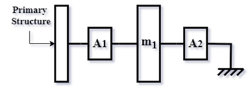
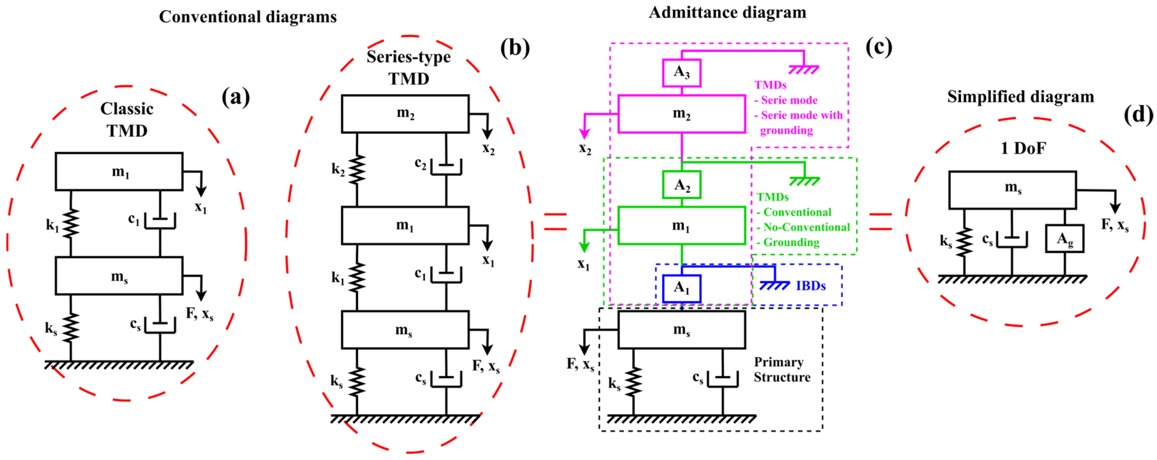
2.1. DVAs’ Simplification Analogy Using the Mechanical Admittance Concept
2.2. Mathematical Modeling of Classical TMD, Series TMD, and Admittance
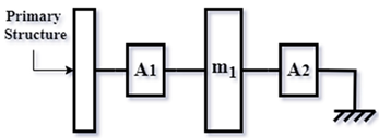
2.3. Global Mechanical Admittance
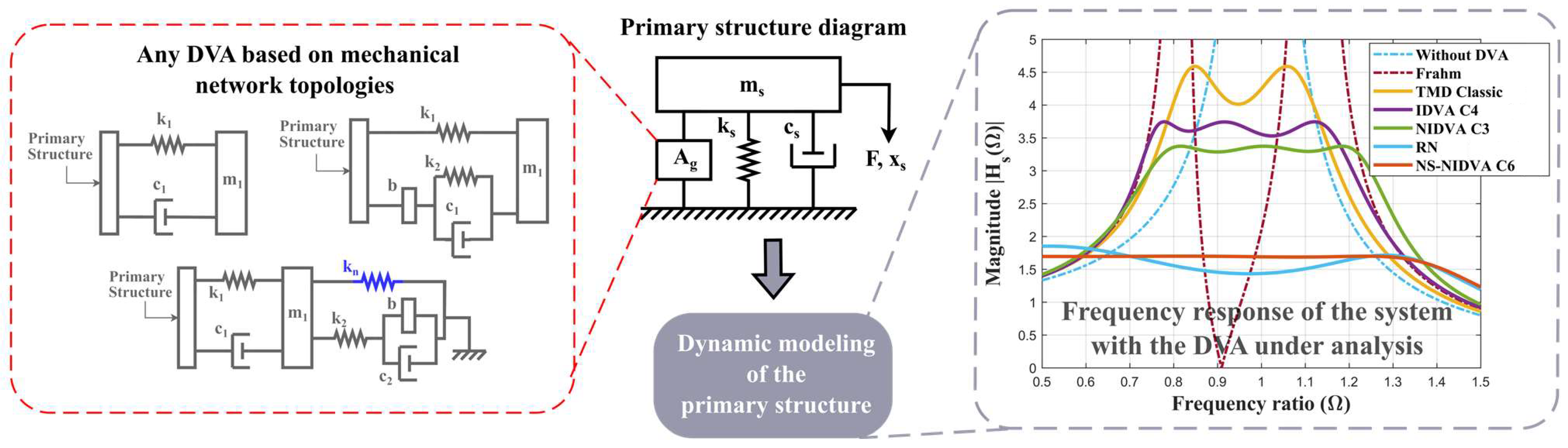
2.4. How to Apply for Global Admittance
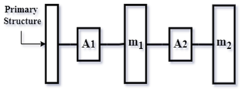
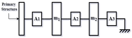
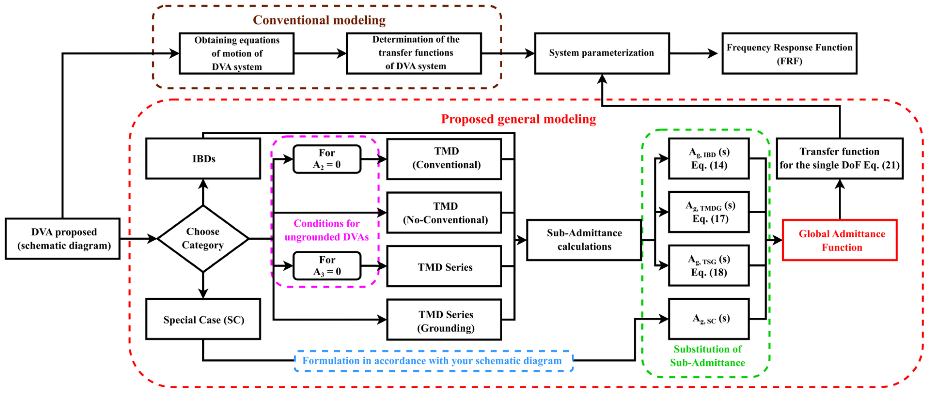
3. Modeling Procedure
3.1. Conventional Modeling and Global Admittance Variances
3.2. Parameterization and FRF
4. Method Implementation
4.1. Selection of the DVAs and Their FRFs
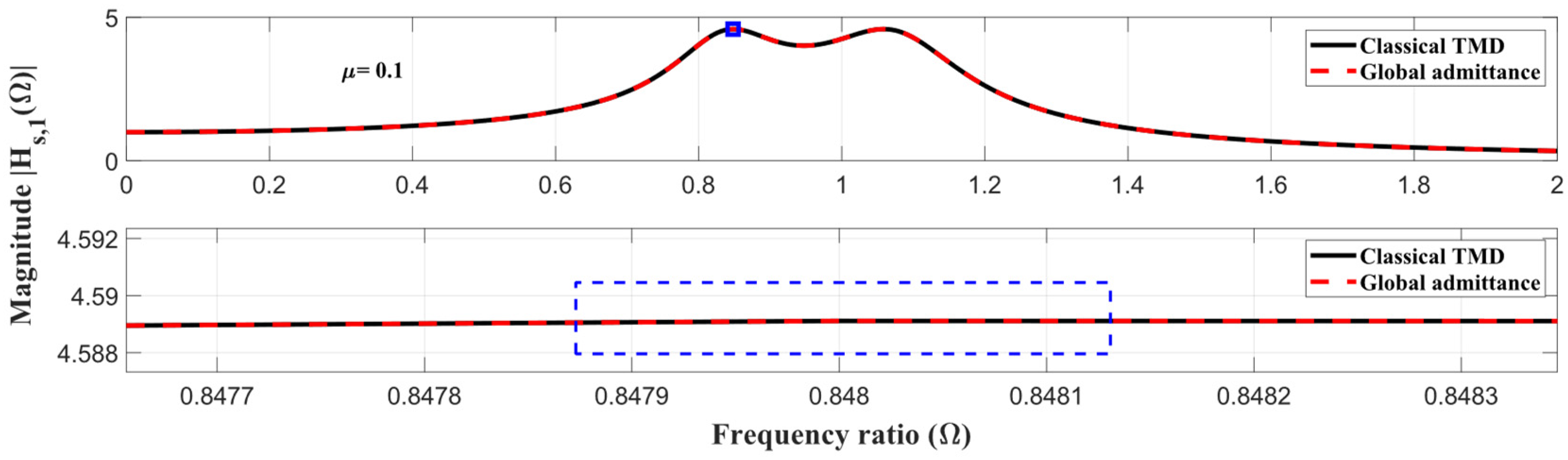
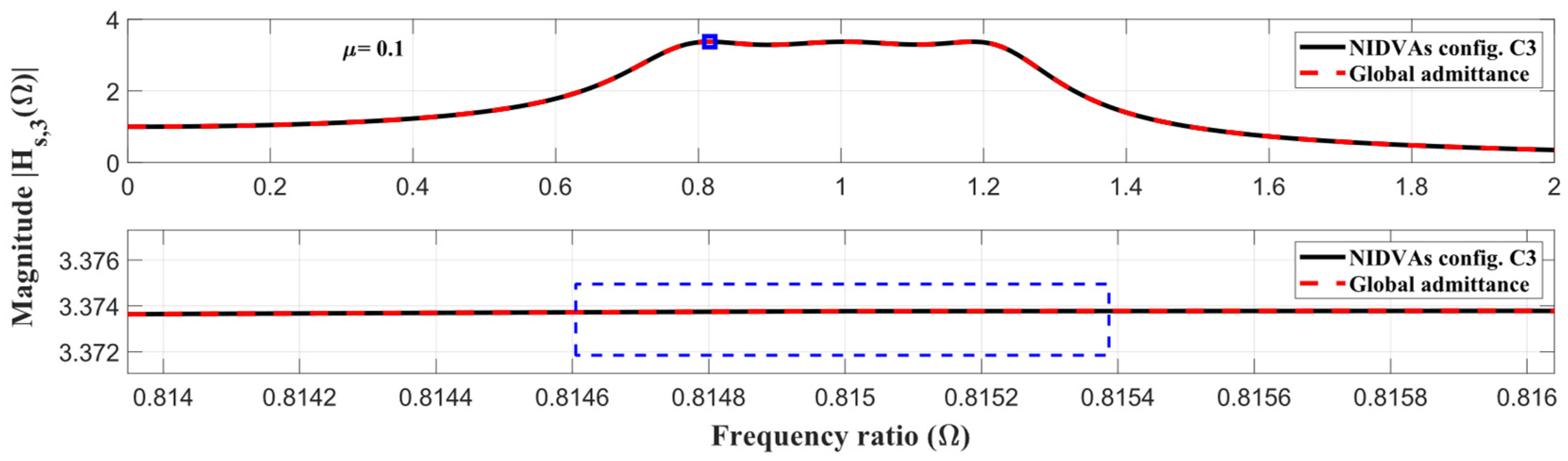
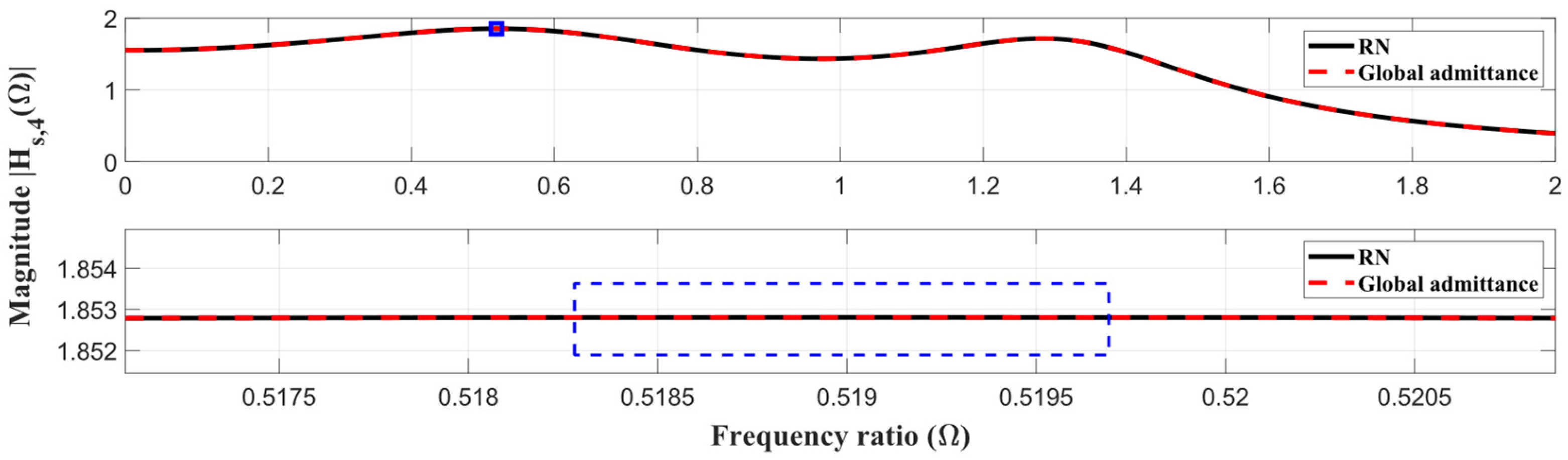
4.2. FRFs Simulation and Result Discussion
5. Conclusions
Author Contributions
Funding
Data Availability Statement
Conflicts of Interest
Appendix A. Sub-Admittance Functions

| Schematic Diagram by Admittance | Associated DVAs | Internal Diagram of | Functions |
|---|---|---|---|
 | (VMD) [56] (2007) | 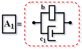 | |
| (TVMD) [57] (2012) | 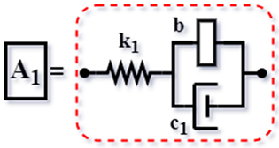 | ||
| TID [58] (2014) |  | ||
| IBDs [25] (2015) | |||
| Config. C2 | 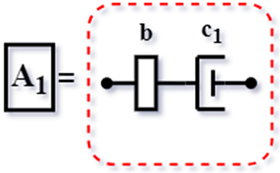 | ||
| Config. C3 | 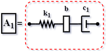 | ||
| Config. C5 | 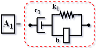 | ||
| Schematic Diagram by Admittance | Associated DVAs | Internal Diagram of | Functions |
|---|---|---|---|
 | Classical TMD [5] (1928) | 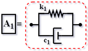 | |
| TMD for Asami [6] (1999) | 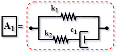 | ||
| TMDI Hu [25] (2015) | |||
| Config. C1 | 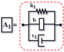 | ||
| Config. C2 | 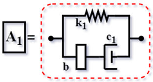 | ||
| Config. C3 | 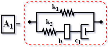 | ||
| Config. C4 |  | ||
| Config. C5 |  | ||
| Config. C6 | 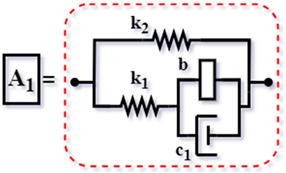 | ||
| IA1 [59] (2018) | 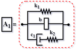 | ||
| Schematic Diagram by Admittance | Associated DVAs | Internal Diagram of | Functions |
|---|---|---|---|
 | TMD for Ren [10] (2001) | 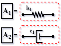 | |
| TMD for Wang [9] (2016) | 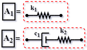 | ||
| TMDI [60] (2014) | 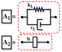 | ||
| WN [61] (2016) | 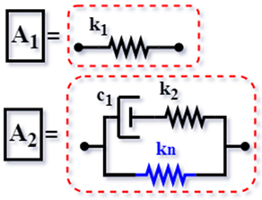 | ||
| RN [54] (2017) | 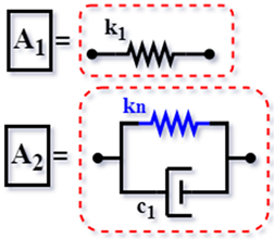 | ||
| IA2 [59] (2018) | 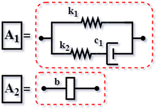 | ||
| IR1 [59] (2018) | 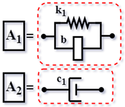 | ||
| IR2 [59] (2018) | 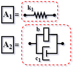 | ||
| AN [62] (2019) | 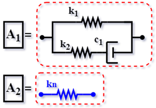 | ||
| WI [62] (2019) |  | ||
 | DN [62] (2019) | 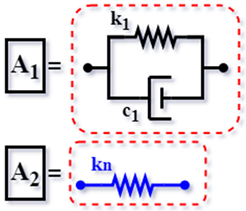 | |
| DIN [62] (2019) |  | ||
| RIN [62] (2019) |  | ||
| AIN [62] (2019) | 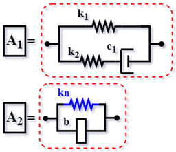 | ||
| WIN [62] (2019) | 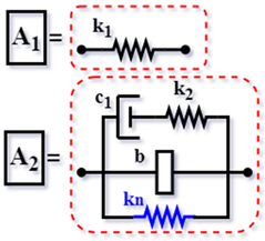 | ||
| NIDVAs [24] (2020) | |||
| Config. C3 | 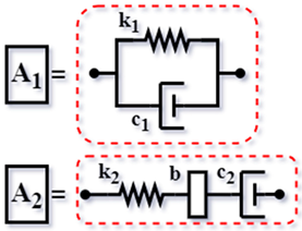 | ||
| Config. C4 | 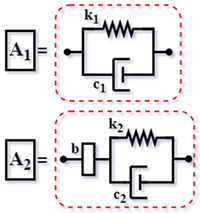 | ||
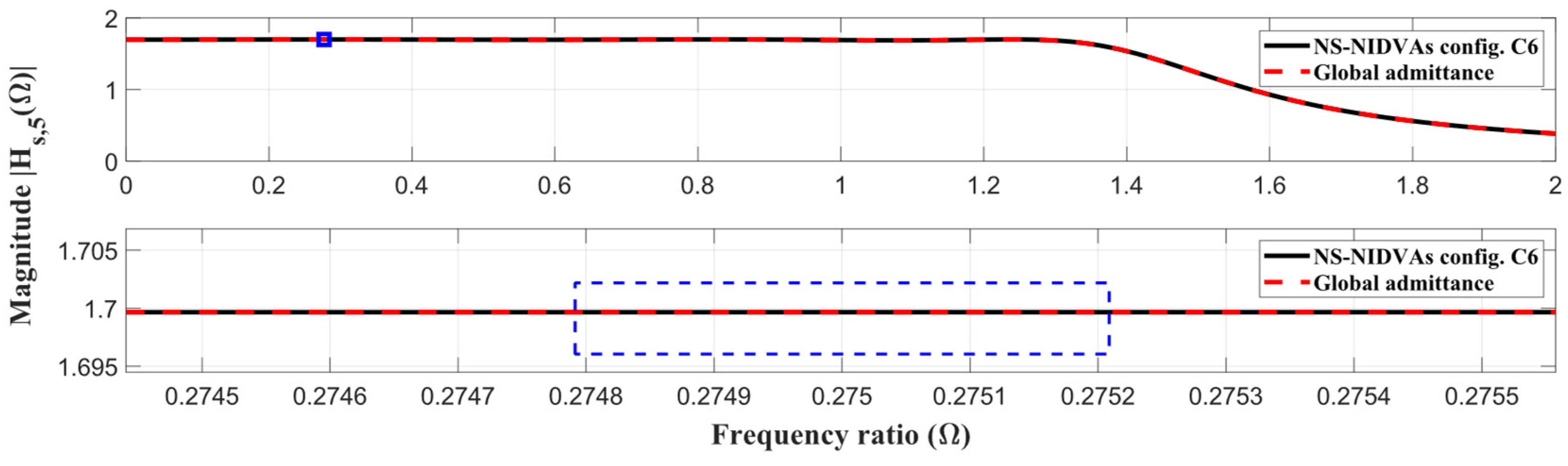
| Config. C6 |  | ||
 | NS-NIDVAs [55] (2021) | ||
| Config. C3 | 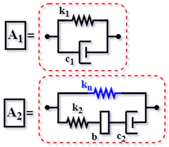 | ||
| Config. C4 | 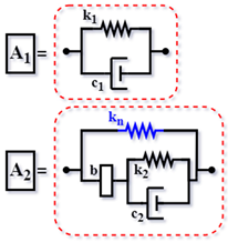 | ||
| Config. C6 | 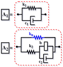 | ||
| TE-type [63] (2023) | 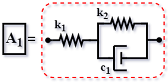 | ||
| TEI-type [63] (2023) |  | ||
| NS-TE-type [63] (2023) | 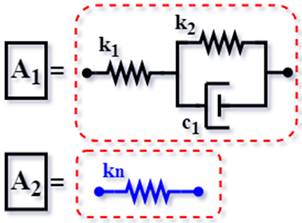 | ||
| NI-TE-type [63] (2023) | 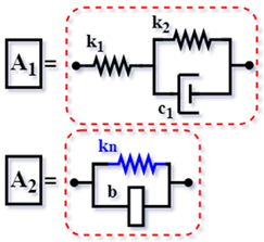 | ||
| Schematic Diagram by Admittance | Associated DVAs | Internal Diagram of | Functions |
|---|---|---|---|
| Based series TMDs | |||
 | TMD series mode [15] (2016) | 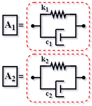 | |
| I-SDTMDI [23] (2019) | 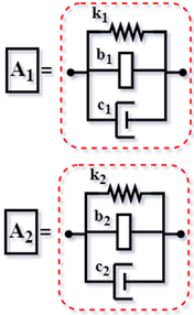 | ||
| TMD series-type with grounding. | |||
 | SDTMDI type II [23] (2019) |  | |
| Especial cases | |||
| Global admittance function (parallel TMD) | |||
 | Parallel TMD [15] (2016) |  | |
| Global admittance function (serial-type TMD with grounding on the primary TMD) | |||
 | SDTMDI type I [23] (2019) | 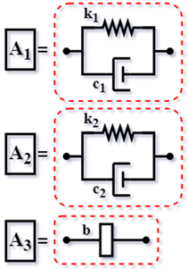 | |
Appendix B. Equations of Motion Based on Mechanical Admittance
Appendix C. Global Admittance Functions
| DVA | Schematic Diagram | Functions Ag(s) |
|---|---|---|
| TMD for Hartog [5] (1928) | 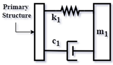 | |
| TMD for Asami [6] (1999) | 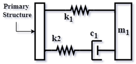 | |
| TMD for Ren [10] (2001) | 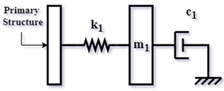 | |
| Viscous mass damper (VMD) [56] (2007) | 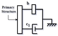 | |
| Tuned viscous mass damper (TVMD) [57] (2012) | 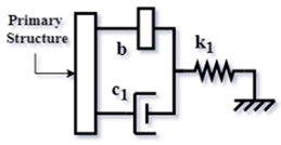 | |
| Tuned inerter damper (TID) [58] (2014) |  | |
| TMDI [60] (2014) | 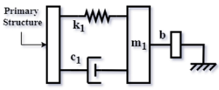 | |
| TMDI for Hu [25] (2015) | ||
| Config. C1 | 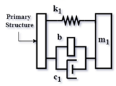 | |
| Config. C2 | 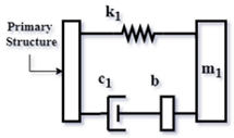 | |
| Config. C3 | 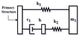 | |
| Config. C4 |  | |
| Config. C5 | 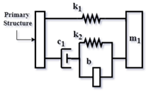 | |
| Config. C6 | 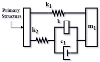 | |
| Inerter-based dampers (IBDs) [25] (2015) | ||
| Config. C2 | 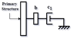 | |
| Config. C3 | 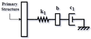 | |
| Config. C5 |  | |
| TMD for Wang [9] (2016) |  | |
| TMD series mode [15] (2016) |  | |
| TMD parallel mode [15] (2016) |  | |
| NS-TMD based on Wang’s TMD (WN) [61] (2016) |  | |
| NS-TMD based on Ren’s TMD (RN) [54] (2017) |  | |
| TMDI type 1 based on Asami’s TMD (AI1) [59] (2018) | 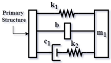 | |
| TMDI type 2 based on Asami’s TMD (AI2) [59] (2018) | 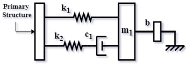 | |
| TMDI type 1 based on Ren’s TMD (RI1) [59] (2018) |  | |
| TMDI type 2 based on Ren’s TMD (RI2) [59] (2018) | 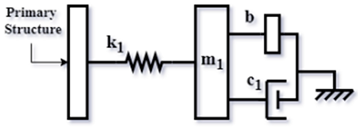 | |
| I-SDTMDI [23] (2019) | 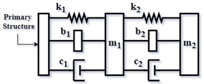 | |
| G-SDTMDI type I [23] (2019) |  | |
| G-SDTMDI type II [23] (2019) |  | |
| NS-TMD based on Hartog’s TMD (DN) [62] (2019) |  | |
| NI-TMD based on Hartog’s TMD (DIN) [62] (2019) |  | |
| NS-TMD based on Asami’s TMD (AN) [62] (2019) |  | |
| NI-TMD based on Asami’s TMD (AIN) [62] (2019) |  | |
| NI-TMD based on Ren’s TMD (RIN) [62] (2019) |  | |
| TMDI based on Wang’s TMD (WI) [62] (2019) |  | |
| NI-TMD based on Wang’s TMD (WIN) [62] (2019) |  | |
| Non-traditional inerter-based dynamic vibration absorber (NIDVAs) [24] (2020) | ||
| Config. C3 | 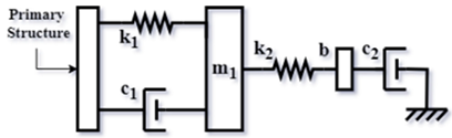 | |
| Config. C4 | 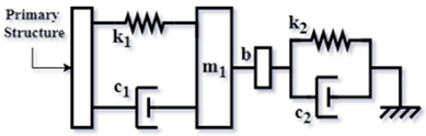 | |
| Config. C6 |  | |
| Negative-stiffness nontraditional inerter-based dynamic vibration absorbers NS-NIDVAs (NS-NIDVAs) [55] (2021) | ||
| Config. C3 | 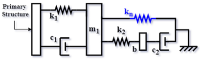 | |
| Config. C4 |  | |
| Config. C6 | 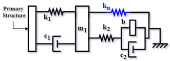 | |
| Three-element DVA model (TE-type) [63] (2023) |  | |
| Three-element DVA model with inerter (TEI-type) [63] (2023) |  | |
| Three-element DVA model with negative stiffness (NS-TE-type) [63] (2023) | 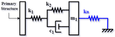 | |
| Three-element DVA model with inerter and negative stiffness (NI-TE-type) [63] (2023) | 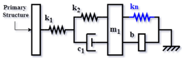 | |
Appendix D. Coefficients Ai, Bi, Ci, and Di for i = 1, 2, …, 5
References
- Pastia, C.; Luca, S.G.; Chira, F.; Roşca, V.O. Structural control systems implemented in civil engineering. Bull. Polytech. Inst. Jassy Constr. Archit. Sect. LI (LV) 2005, 76–80. [Google Scholar]
- Constantinou, M.; Soong, T.; Dargush, G. Passive Energy Dissipation Systems for Structural Design and Retrofit, Monograph No. 1; Multidisciplinary Center for Earthquake Engineering Research: Buffalo, NY, USA, 1998; pp. 9–62. [Google Scholar]
- Elias, S.; Matsagar, V. Research developments in vibration control of structures using passive tuned mass dampers. Annu. Rev. Control 2017, 44, 129–156. [Google Scholar] [CrossRef]
- Frahm, H. Device for Damping Vibrations of Bodies. United States Patent Appl. 0989958, April 15, 1911. Available online: https://www.freepatentsonline.com/0989958.html (accessed on 20 December 2024).
- Ormondroyd, J.; Den Hartog, J.P. The Theory of the Dynamic Vibration Absorber. Trans. Am. Soc. Mech. Eng. 1928, 49–50, 021007. [Google Scholar] [CrossRef]
- Asami, T.; Nishihara, O. Analytical and Experimental Evaluation of an Air Damped Dynamic Vibration Absorber: Design Optimizations of the Three-Element Type Model. J. Vib. Acoust. 1999, 121, 334–342. [Google Scholar] [CrossRef]
- Nishihara, O. Exact Optimization of a Three-Element Dynamic Vibration Absorber: Minimization of the Maximum Amplitude Magnification Factor. J. Vib. Acoust. 2019, 141, 011001. [Google Scholar] [CrossRef]
- Batou, A.; Adhikari, S. Optimal parameters of viscoelastic tuned-mass dampers. J. Sound Vib. 2019, 445, 17–28. [Google Scholar] [CrossRef]
- Wang, X.; Shen, Y.; Yang, S. H∞ optimization of the grounded three-element type dynamic vibration absorber. J. Dyn. Control 2016, 14, 448–453. [Google Scholar] [CrossRef]
- Ren, M.Z. A variant design of the dynamic vibration absorber. J. Sound Vib. 2001, 245, 762–770. [Google Scholar] [CrossRef]
- Cheung, Y.L.; Wong, W.O. H2 optimization of a non-traditional dynamic vibration absorber for vibration control of structures under random force excitation. J. Sound Vib. 2011, 330, 1039–1044. [Google Scholar] [CrossRef]
- Cheung, Y.L.; Wong, W.O. H-infinity optimization of a variant design of the dynamic vibration absorber—Revisited and new results. J. Sound Vib. 2011, 330, 3901–3912. [Google Scholar] [CrossRef]
- Kim, S.-Y.; Lee, C.-H. Optimum design of linear multiple tuned mass dampers subjected to white-noise base acceleration considering practical configurations. Eng. Struct. 2018, 171, 516–528. [Google Scholar] [CrossRef]
- Asami, T. Exact Algebraic Solution of an Optimal Double-Mass Dynamic Vibration Absorber Attached to a Damped Primary System. J. Vib. Acoust. 2019, 141, 051013. [Google Scholar] [CrossRef]
- Asami, T. Optimal Design of Double-Mass Dynamic Vibration Absorbers Arranged in Series or in Parallel. J. Vib. Acoust. 2016, 139, 011015. [Google Scholar] [CrossRef]
- Wang, C.; Brown, J.D.; Singh, A.; Moore, K.J. A two-dimensional nonlinear vibration absorber using elliptical impacts and sliding. Mech. Syst. Signal Process. 2023, 189, 110068. [Google Scholar] [CrossRef]
- Geng, X.-F.; Ding, H.; Ji, J.-C.; Wei, K.-X.; Jing, X.-J.; Chen, L.-Q. A state-of-the-art review on the dynamic design of nonlinear energy sinks. Eng. Struct. 2024, 313, 118228. [Google Scholar] [CrossRef]
- Yang, Y.; Dai, W.; Liu, Q. Design and implementation of two-degree-of-freedom tuned mass damper in milling vibration mitigation. J. Sound Vib. 2015, 335, 78–88. [Google Scholar] [CrossRef]
- Ma, W.; Yang, Y.; Yu, J. General routine of suppressing single vibration mode by multi-DOF tuned mass damper: Application of three-DOF. Mech. Syst. Signal Process. 2019, 121, 77–96. [Google Scholar] [CrossRef]
- Schmelzer, B.; Oberguggenberger, M.; Adam, C. Efficiency of tuned mass dampers with uncertain parameters on the performance of structures under stochastic excitation. Proc. Inst. Mech. Eng. Part O J. Risk Reliab. 2010, 224, 297–308. [Google Scholar] [CrossRef]
- Smith, M. Synthesis of mechanical networks: The inerter. IEEE Trans. Autom. Control. 2002, 47, 1648–1662. [Google Scholar] [CrossRef]
- Platus, D. Negative-Stiffness-Mechanism Vibration Isolation Systems (SPIE Technical: OPTCON ’91); SPIE: Bellingham, WA, USA, 1992. [Google Scholar]
- Zhou, S.; Jean-Mistral, C.; Chesne, S. Influence of inerters on the vibration control effect of series double tuned mass dampers: Two layouts and analytical study. Struct. Control Health Monit. 2019, 26, e2414. [Google Scholar] [CrossRef]
- Barredo, E.; Larios, J.M.; Colín, J.; Mayén, J.; Flores-Hernández, A.; Arias-Montiel, M. A novel high-performance passive non-traditional inerter-based dynamic vibration absorber. J. Sound Vib. 2020, 485, 115583. [Google Scholar] [CrossRef]
- Hu, Y.; Chen, M.Z. Performance evaluation for inerter-based dynamic vibration absorbers. Int. J. Mech. Sci. 2015, 99, 297–307. [Google Scholar] [CrossRef]
- Cao, L.; Li, C. Tuned tandem mass dampers-inerters with broadband high effectiveness for structures under white noise base excitations. Struct. Control Health Monit. 2019, 26, e2319. [Google Scholar] [CrossRef]
- Javidialesaadi, A.; Wierschem, N.E. An inerter-enhanced nonlinear energy sink. Mech. Syst. Signal Process. 2019, 129, 449–454. [Google Scholar] [CrossRef]
- Cheng, Z.; Palermo, A.; Shi, Z.; Marzani, A. Enhanced tuned mass damper using an inertial amplification mechanism. J. Sound Vib. 2020, 475, 115267. [Google Scholar] [CrossRef]
- Wang, Q.; Tiwari, N.D.; Qiao, H.; Wang, Q. Inerter-based tuned liquid column damper for seismic vibration control of a single-degree-of-freedom structure. Int. J. Mech. Sci. 2020, 184, 105840. [Google Scholar] [CrossRef]
- Zhao, Z.; Zhang, R.; Jiang, Y.; Pan, C. A tuned liquid inerter system for vibration control. Int. J. Mech. Sci. 2019, 164, 105171. [Google Scholar] [CrossRef]
- Gonzalez-Buelga, A.; Clare, L.R.; Neild, S.A.; Burrow, S.G.; Inman, D.J. An electromagnetic vibration absorber with harvesting and tuning capabilities. Struct. Control Health Monit. 2015, 22, 1359–1372. [Google Scholar] [CrossRef]
- Xiuchang, H.; Zhiwei, S.; Hongxing, H. Optimal parameters for dynamic vibration absorber with negative stiffness in controlling force transmission to a rigid foundation. Int. J. Mech. Sci. 2019, 152, 88–98. [Google Scholar] [CrossRef]
- Huang, X.; Su, Z.; Hua, H. Application of a dynamic vibration absorber with negative stiffness for control of a marine shafting system. Ocean Eng. 2018, 155, 131–143. [Google Scholar] [CrossRef]
- Shen, Y.; Xing, Z.; Yang, S.; Sun, J. Parameters optimization for a novel dynamic vibration absorber. Mech. Syst. Signal Process. 2019, 133, 106282. [Google Scholar] [CrossRef]
- Su, N.; Chen, Z.; Zeng, C.; Xia, Y.; Bian, J. Concise analytical solutions to negative-stiffness inerter-based DVAs for seismic and wind hazards considering multi-target responses. Earthq. Eng. Struct. Dyn. 2024, 53, 3820–3858. [Google Scholar] [CrossRef]
- Jin, X.; Chen, M.Z.; Huang, Z. Minimization of the beam response using inerter-based passive vibration control configurations. Int. J. Mech. Sci. 2016, 119, 80–87. [Google Scholar] [CrossRef]
- Kaveh, A.; Farzam, M.F.; Jalali, H.H. Statistical seismic performance assessment of tuned mass damper inerter. Struct. Control Health Monit. 2020, 27, e2602. [Google Scholar] [CrossRef]
- Shen, W.; Niyitangamahoro, A.; Feng, Z.; Zhu, H. Tuned inerter dampers for civil structures subjected to earthquake ground motions: Optimum design and seismic performance. Eng. Struct. 2019, 198, 109470. [Google Scholar] [CrossRef]
- Hu, Y.; Wang, J.; Chen, M.Z.; Li, Z.; Sun, Y. Load mitigation for a barge-type floating offshore wind turbine via inerter-based passive structural control. Eng. Struct. 2018, 177, 198–209. [Google Scholar] [CrossRef]
- Zhang, Z.; Fitzgerald, B. Tuned mass-damper-inerter (TMDI) for suppressing edgewise vibrations of wind turbine blades. Eng. Struct. 2020, 221, 110928. [Google Scholar] [CrossRef]
- Shen, Y.; Chen, L.; Yang, X.; Shi, D.; Yang, J. Improved design of dynamic vibration absorber by using the inerter and its application in vehicle suspension. J. Sound Vib. 2016, 361, 148–158. [Google Scholar] [CrossRef]
- Ma, R.; Bi, K.; Hao, H. Mitigation of heave response of semi-submersible platform (SSP) using tuned heave plate inerter (THPI). Eng. Struct. 2018, 177, 357–373. [Google Scholar] [CrossRef]
- Lazar, I.; Neild, S.; Wagg, D. Vibration suppression of cables using tuned inerter dampers. Eng. Struct. 2016, 122, 62–71. [Google Scholar] [CrossRef]
- Rahimi, F.; Aghayari, R.; Samali, B. Application of Tuned Mass Dampers for Structural Vibration Control: A State-of-the-art Review. Civ. Eng. J. 2020, 6, 1622–1651. [Google Scholar] [CrossRef]
- Ma, R.; Bi, K.; Hao, H. Inerter-based structural vibration control: A state-of-the-art review. Eng. Struct. 2021, 243, 112655. [Google Scholar] [CrossRef]
- AChaudhary, S.; Nandanwar, Y.N.; Mungale, N.G. A review on optimization of design of tuned mass dampers. J. Phys. Conf. Ser. 2021, 1913, 012003. [Google Scholar] [CrossRef]
- Yang, F.; Sedaghati, R.; Esmailzadeh, E. Vibration suppression of structures using tuned mass damper technology: A state-of-the-art review. J. Vib. Control 2022, 28, 812–836. [Google Scholar] [CrossRef]
- Nishihara, O.; Asami, T. Closed-Form Solutions to the Exact Optimizations of Dynamic Vibration Absorbers (Minimizations of the Maximum Amplitude Magnification Factors). J. Vib. Acoust. 2002, 124, 576–582. [Google Scholar] [CrossRef]
- Zilletti, M.; Elliott, S.J.; Rustighi, E. Optimisation of dynamic vibration absorbers to minimise kinetic energy and maximise internal power dissipation. J. Sound Vib. 2012, 331, 4093–4100. [Google Scholar] [CrossRef]
- Warburton, G.B. Optimum absorber parameters for various combinations of response and excitation parameters. Earthq. Eng. Struct. Dyn. 1982, 10, 381–401. [Google Scholar] [CrossRef]
- Su, N.; Chen, Z.; Xia, Y.; Bian, J. Hybrid analytical H-norm optimization approach for dynamic vibration absorbers. Int. J. Mech. Sci. 2024, 264, 108796. [Google Scholar] [CrossRef]
- Zhao, Z.; Chen, Q.; Zhang, R.; Pan, C.; Jiang, Y. Energy dissipation mechanism of inerter systems. Int. J. Mech. Sci. 2020, 184, 105845. [Google Scholar] [CrossRef]
- Miller, D.; Crawley, E.; Ward, B. Inertial actuator design for maximum passive and active energy dissipation in flexible space structures. In Proceedings of the 26th Structures, Structural Dynamics, and Materials Conference, Orlando, FL, USA, 15–17 April 1985. [Google Scholar]
- Shen, Y.; Peng, H.; Li, X.; Yang, S. Analytically optimal parameters of dynamic vibration absorber with negative stiffness. Mech. Syst. Signal Process. 2017, 85, 193–203. [Google Scholar] [CrossRef]
- Barredo, E.; Rojas, G.L.; Mayén, J.; Flores-Hernández, A. Innovative negative-stiffness inerter-based mechanical networks. Int. J. Mech. Sci. 2021, 205, 106597. [Google Scholar] [CrossRef]
- Hwang, J.-S.; Kim, J.; Kim, Y.-M. Rotational inertia dampers with toggle bracing for vibration control of a building structure. Eng. Struct. 2007, 29, 1201–1208. [Google Scholar] [CrossRef]
- Ikago, K.; Saito, K.; Inoue, N. Seismic control of single-degree-of-freedom structure using tuned viscous mass damper. Earthq. Eng. Struct. Dyn. 2012, 41, 453–474. [Google Scholar] [CrossRef]
- Lazar, I.F.; Neild, S.; Wagg, D. Using an inerter-based device for structural vibration suppression. Earthq. Eng. Struct. Dyn. 2014, 43, 1129–1147. [Google Scholar] [CrossRef]
- Wang, X.; Liu, X.; Shan, Y.; Shen, Y.; He, T. Analysis and Optimization of the Novel Inerter-Based Dynamic Vibration Absorbers. IEEE Access 2018, 6, 33169–33182. [Google Scholar] [CrossRef]
- Marian, L.; Giaralis, A. Optimal design of a novel tuned mass-damper–inerter (TMDI) passive vibration control configuration for stochastically support-excited structural systems. Probabilistic Eng. Mech. 2014, 38, 156–164. [Google Scholar] [CrossRef]
- Shen, Y.; Wang, X.; Yang, S.; Xing, H. Parameters Optimization for a Kind of Dynamic Vibration Absorber with Negative Stiffness. Math. Probl. Eng. 2016, 2016, 9624325. [Google Scholar] [CrossRef]
- Wang, X.; He, T.; Shen, Y.; Shan, Y.; Liu, X. Parameters optimization and performance evaluation for the novel inerter-based dynamic vibration absorbers with negative stiffness. J. Sound Vib. 2019, 463, 114941. [Google Scholar] [CrossRef]
- Gao, T.; Li, J.; Zhu, S.; Yang, X.; Zhao, H. H∞ Optimization of Three-Element-Type Dynamic Vibration Absorber with Inerter and Negative Stiffness Based on the Particle Swarm Algorithm. Entropy 2023, 25, 1048. [Google Scholar] [CrossRef]

| Parameter | Definition | Description |
|---|---|---|
| Common parameters | DVA-to-primary mass ratio | |
| Natural frequency of the primary system | ||
| Natural frequency of the DVA | ||
| Undamped natural frequency DVA-to-primary system | ||
| Forced frequency ratio | ||
| Damping ratio for the primary structure | ||
| Damping ratio for the DVA | ||
| Recommended parameters by the authors | ||
| Classical TMD [5] | Damping ratio recommended by the authors | |
| TMDI Config. C4 [25] | Inertance-to-DVA mass ratio | |
| Natural frequency of the inerter-based mechanical networks (IMN) | ||
| Undamped natural frequency IMN-to-DVA ratio | ||
| NIDVA Config. C3 [24] | Common parameters with TMDI | |
| Damping ratio for inerter | ||
| NS-TMD based on Ren’s TMD (RN) [54] | Negative stiffness-to-DVA stiffness ratio | |
| NS-NIDVA Config. C6 [55] | Standard parameters with TMDI and RN | |
| IMN-to-DVA stiffness ratio | ||
| Damping ratio recommended by the authors |
| i | DVA | Schematic Diagram | Global Admittance Function Connection Ratio () |
|---|---|---|---|
| 1. | Classical TMD Hartog and Ormondroyd [5] | 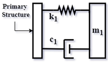 | |
| 2. | TMDI Config. C4 Hu and Chen [25] | 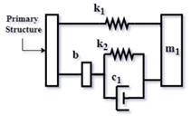 | |
| 3. | NIDVAs Config. C3 Barredo et al. [24] | 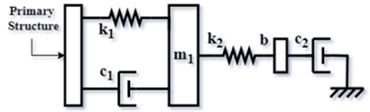 | Where: |
| 4. | RN Shen et al. [54] | 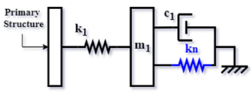 | |
| 5. | NS-NIDVAs Config. C6 Barredo et al. [55] |  | Where: |
| DVA | Norm | ||||||||
|---|---|---|---|---|---|---|---|---|---|
| Classical TMD [48] | 0.1 | — | 0.909058 | — | — | 0.168603 | — | — | 4.589166 |
| TMDI Config. C4 [25] | 0.1 | 0.193000 | 0.949900 | 0.901300 | — | 0.050500 | — | — | 3.744480 |
| NIDVAs Config. C3 [24] | 0.1 | 0.291768 | 1.022202 | 0.950684 | — | 0 | 0.636188 | — | 3.373789 |
| RN [54] | 0.1 | — | 1.697077 | — | −0.552786 | 0.334370 | — | — | 1.846700 |
| NS-NIDVA Config. C6 [55] | 0.1 | 0.316594 | 1.454698 | — | −0.659952 | 0 | 0.305162 | 0.486543 | 1.699654 |
Disclaimer/Publisher’s Note: The statements, opinions and data contained in all publications are solely those of the individual author(s) and contributor(s) and not of MDPI and/or the editor(s). MDPI and/or the editor(s) disclaim responsibility for any injury to people or property resulting from any ideas, methods, instructions or products referred to in the content. |
© 2025 by the authors. Licensee MDPI, Basel, Switzerland. This article is an open access article distributed under the terms and conditions of the Creative Commons Attribution (CC BY) license (https://creativecommons.org/licenses/by/4.0/).
Share and Cite
Mazón-Valadez, C.; Barredo, E.; Colín-Ocampo, J.; Pérez-Molina, J.A.; Pérez-Vigueras, D.; Mazón-Valadez, E.E.; Barrera-Sánchez, A. Global Admittance: A New Modeling Approach to Dynamic Performance Analysis of Dynamic Vibration Absorbers. Vibration 2025, 8, 19. https://doi.org/10.3390/vibration8020019
Mazón-Valadez C, Barredo E, Colín-Ocampo J, Pérez-Molina JA, Pérez-Vigueras D, Mazón-Valadez EE, Barrera-Sánchez A. Global Admittance: A New Modeling Approach to Dynamic Performance Analysis of Dynamic Vibration Absorbers. Vibration. 2025; 8(2):19. https://doi.org/10.3390/vibration8020019
Chicago/Turabian StyleMazón-Valadez, Cuauhtémoc, Eduardo Barredo, Jorge Colín-Ocampo, Javier A. Pérez-Molina, Demetrio Pérez-Vigueras, Ernesto E. Mazón-Valadez, and Agustín Barrera-Sánchez. 2025. "Global Admittance: A New Modeling Approach to Dynamic Performance Analysis of Dynamic Vibration Absorbers" Vibration 8, no. 2: 19. https://doi.org/10.3390/vibration8020019
APA StyleMazón-Valadez, C., Barredo, E., Colín-Ocampo, J., Pérez-Molina, J. A., Pérez-Vigueras, D., Mazón-Valadez, E. E., & Barrera-Sánchez, A. (2025). Global Admittance: A New Modeling Approach to Dynamic Performance Analysis of Dynamic Vibration Absorbers. Vibration, 8(2), 19. https://doi.org/10.3390/vibration8020019