

From Scalar Clouds to Rotating Hairy Black Holes

1
Instituto de Ciencias Nucleares, Universidad Nacional Autónoma de México, A.P. 70-543, Mexico City 04510, Mexico
2
Laboratoire Univers et Théories, Observatoire de Paris, Université PSL, Université Paris Cité, UMR 8102 CNRS, F-92190 Meudon, France
*
Author to whom correspondence should be addressed.
Particles 2024, 7(1), 1-24; https://doi.org/10.3390/particles7010001
Submission received: 2 October 2023
/
Revised: 31 October 2023
/
Accepted: 30 November 2023
/
Published: 21 December 2023
(This article belongs to the Special Issue Selected Papers from “Testing Gravity 2023”)
Abstract
:First, we review the solutions of a complex-valued scalar field, termed scalar clouds, with and without electric charge, when coupled to a rotating Kerr–Newman (electrically charged) or Kerr (neutral) black hole (BH), respectively. To this aim, we determine the conditions and parameters that characterize the existence of solutions that represent bound states, with an energy-momentum tensor that respect the symmetries of the underlying spacetimes, even if the backreaction of the field is not taken into account at this stage. In particular, we show that in the extremal Kerr scenario the cloud solutions exist only when the mass of the BH satisfies certain bounds, which are obtained by analyzing an effective potential associated with the radial dependency of the scalar clouds that leads to a Schrödinger-like equation. Second, when the backreaction of the field in the spacetime is taken into account, we present a family of stationary, axisymmetric and asymptotically flat solutions of the Einstein–Klein–Gordon system that represent genuine rotating hairy black holes (RHBHs) and provide different values of some global quantities associated with them, such as the Komar mass and the Komar angular momentum. We also compute RHBH solutions with nodes in the radial part of the scalar field and also for a higher azimuthal number m.
1. Introduction
Black holes (BHs) represent some of the most interesting and relevant astrophysical objects as predicted by Einstein’s general relativity. Since the first detection of gravitational waves (GWs) by the LIGO-VIRGO collaboration [1] (today LIGO-VIRGO-KAGRA), such objects are no longer in the realm of theoretical speculations, but they became an accepted piece of reality in our universe: the best explanation for the sources of such GWs is provided by the inspiriling and the merger of two BHs (and sometimes of two neutron stars) followed by the ringdown of a remaining Kerr BH. This interpretation has been the result of exquisite simulations developed by the numerical relativity community, specially during the past two decades. Moreover, the images obtained by the Event Horizon Telescope (EHT) from the centers of galaxy M87 [2] and our own galaxy [3] are consistent with the hypothesis of light emitted from accretion discs around BHs located at such centers, which are then distorted by their corresponding gravitational fields before reaching the telescope.
At a fundamental level, the simplest BHs are characterized by three parameters, their mass (M), electric charge (Q) and angular momentum (J) (no-hair conjecture) [4,5], and are a consequence of solving the Einstein field equations in a vacuum or with an electromagnetic field under suitable symmetries and by imposing regularity and asymptotic conditions. These studies led to the BH uniqueness theorems [6,7,8,9,10,11,12,13], which several years later were complemented by several no-hair theorems [14,15,16,17,18,19,20], showing that quantities no other than the above three parameters characterize a BH.
In recent years, the no-hair conjecture has proven to be false when nonlinear field theoretical models have been considered [21,22,23]. However, most if not all the hairy BH solutions within those models (the majority of which have been obtained in static and spherically symmetric scenarios) have proven to be unstable with respect to linear perturbations. Surprisingly, in 2014, Herdeiro and Radu [24,25] discovered numerically that rotating hairy BH solutions of the Einstein–(complex)Klein–Gordon system could exist if the assumptions of staticity and spherical symmetry are dropped—conditions that are required by some of the existing no-hair theorems [19]. These authors also showed that if the background of a Kerr spacetime was fixed, the solutions of the (complex) Klein–Gordon system also exist—solutions that are referred to as clouds. This result extends a previous analysis by Hod for the existence of exact cloud solutions around an extremal Kerr spacetime [26]. More recently, those solutions have been generalized to include electric charges [27,28,29,30,31,32]. Further studies have put forward heuristic analyses that allow us to understand the existence of such solutions on simple grounds [31,32,33] and show why the no-hair theorems cannot be extended precisely when rotation and axisymmetry are taken into account in the assumptions. These discoveries have also motivated the analysis of analogue systems in fluids and other media that can mimic scalar clouds around acoustic horizons [34,35,36]. Moreover, scalar clouds have also been analyzed in other types of exotic BH backgrounds [37,38,39,40].
In this paper, we report several neutral and electrically charged (numerical) cloud solutions of the Klein–Gordon equation in the background of Kerr and Kerr–Newman spacetimes. In addition, we show an important connection between an effective gravitational potential (associated with the clouds and the backgrounds) and the possible values admitted by the BH parameters for the cloud (bound-state) solutions to exist, notably, in the extremal BH scenarios. Finally, based on a recent analysis that employs spectral methods [41], we also report new genuine rotating hairy BH solutions of the Herdeiro–Radu type by solving numerically the full Einstein–Klein–Gordon system under the assumptions of axisymmetry, stationarity, circularity and asymptotic flatness by taking into account the backreaction of the scalar field in the spacetime and by considering nodes in the radial part of the field and also higher values for the azimuthal number m.
2. Scalar Clouds around Subextremal BHs
2.1. Charged Scalar Clouds
In this and the following section, we consider a (test) massive, complex and charged scalar field around a Kerr–Newman (KN) BH, which in Boyer–Lindquist coordinates is described by the following spacetime metric,
where
and
where the parameters M, a and Q are the mass, the angular momentum per mass unit and the electric charge associated with the KNBH, respectively.
In this spacetime we can identify the presence of two horizons located at
The horizon at corresponds to the BH event horizon, while at there is an inner Cauchy horizon. A particular case obtained from the above scenario is the Kerr BH associated with a rotating neutral BH, with . In this section, we focus only on the subextremal BH scenarios where and . The extremal ones where and are discussed in subsequent sections.
The energy-momentum tensor (EMT) associated with the scalar field that is studied in relation with the scalar clouds and rotating hairy BHs is given by
where the operator
is the covariant derivative associated with the gauge field , which for a KNBH is given by
and the constant q is the electric charge or gauge coupling for the scalar field . The operator corresponds to the covariant derivative compatible with the metric, in this case, the KN metric. For our study, we focus only on the following potential
which is associated with a massive but free field with mass . Neutral scalar clouds around a Kerr BH are found when .
The dynamics of the charged and massive scalar field are provided by the Klein–Gordon (KG) equation coupled to gravity and the electromagnetic potential:
Because we are interested in finding bound states for in the domain of outer communication (DOC) of the KNBH, including the horizon, we consider the following ansatz with temporal and angular dependence in the form
where is the frequency of the scalar field and m is an integer number. This is the most general form that we can choose such that the EMT (5) respects the symmetries of the KN spacetime (see also Section Global Quantities).
We also impose the zero-flux condition at the BH horizon to ensure the existence of boson clouds [24,25,29,30,32]:
where [42]
is the helical Killing vector field given in terms of the timelike Killing field and the axial Killing field , which are associated with the time and axial symmetries of the background spacetime. The parameter represents the angular velocity of the BH horizon, which in this case is given by
From (11) and Equations (7), (10) and (12), we obtain the following condition:
Assuming that in general , we conclude that the frequency is given in terms of the BH properties at the horizon:
where
is the electric potential at the horizon defined in terms of the helical Killing field, and is the area of the BH event horizon (cf. Ref. [43]). In the context of a neutral Kerr BH, the frequency (15) is called the synchronicity condition [24,25] .
When replacing the scalar field ansatz (10) in the KG Equation (9), we find that the function is separable and can be written as the product of two functions that depend on the coordinates r and , respectively, which allows us to expand the field in modes of the following form
where the angular functions (the spheroidal harmonics) obey the following equation
and are the separation constants () given by
which connects the angular and radial parts of the Klein–Gordon equation and ensures that the angular functions are regular on the axis of symmetry. The number l is a non-negative integer, and the integer n () labels the number of nodes in the radial function . The expansion coefficients can be found in Ref. [44].
2.2. Boundary Conditions
In order to solve the Teukolsky radial Equation (20), we impose the following regularity conditions for the first and second derivatives at the horizon (see Ref. [32] for more details):
and
These regularity conditions are valid in the subextremal scenarios . In the extremal BH cases , these derivatives blow up, and thus, a different strategy is devised to construct cloud solutions numerically [32] (see Appendix A and Appendix B). These remarks apply also for the neutral scalar clouds considered in Section 2.3 below.
Figure 1 shows some solutions to the radial Teukolsky Equation (20) for the integers and , which satisfy the above regularity conditions and vanish asymptotically. These bound-state solutions are found numerically from a fourth-order Runge–Kutta integrator accompanied by a shooting method. During the numerical process, we have fixed the values , Q, and q for a given set of quantum numbers . The shooting method allows us to find the optimal value for the (rotation parameter) a such that the scalar field vanishes exponentially away from the BH. This amounts to finding the corresponding eigenvalue leading to the bound states for the field in the KN background.
Figure 2 shows the existence lines associated with the charged scalar clouds around a KNBH with electric charge and integers and . Our results are compatible with those reported in the past [29].
Figure 3 depicts other solutions for the radial functions when fixing the location of the event horizon but varying the KNBH electric charge Q. We see that when the electric charge increases, the rotation parameter a decreases. Thus, we conclude that the larger the electrical charge Q, the slower the BH rotates in order for the scalar field to keep the balance around the BH. However, note that when this happens the amplitude of the radial function also increases. Thus, one cannot find a finite (continuous) smooth radial function with and with a finite charge Q. This is because there exist no regular clouds in the background of a Reissner–Nordstrom BH with a massive but free scalar field [31].
Figure 4 shows solutions for the radial functions taking [46]. It is worth noting that when one fixes a set of parameters of the system like , one finds that there exist two optimal values of a (as well as M) that allow for the existence of charged scalar clouds, as shown in Figure 4.
On the other hand, based on the numerical results, we observe a correlation between the optimal values of the parameter a and the sign of the scalar field charge . For instance, taking and , we obtain ; however, for the same value of but (i.e., q with the opposite sign), we find that the optimal value is (i.e., a has the opposite sign). This result can be seen as a consequence of the symmetry of the radial Teukolsky Equation (20) under the transformation [47] or .
2.3. Neutral Scalar Clouds
A particular case of the previous scenario corresponds to the neutral scalar clouds () in the background of a Kerr BH (), which is described by the metric (1), with
In this case, the event horizon () and Cauchy horizon () take the form
respectively. For the neutral scalar field , the Klein–Gordon Equation (9) reduces to
and the radial Teukolsky equation becomes
where
and
Given the form of the frequencies and (15) for the Kerr and KN scenarios, respectively, we see that the corresponding quantities and (21) that appear in the radial equations both vanish at their corresponding event horizon .
The angular part of the neutral scalar field in this case satisfies the same angular equation associated with the spheroidal harmonics (18) that appears in the KN scenario, except that is replaced by . To solve the radial Equation (27) in this scenario, we impose the following regularity conditions at the horizon (see Ref. [33] for more details),
and
which can be obtained from Equations (22) and (23) taking , respectively.
Figure 6 shows the existence lines associated with the neutral scalar clouds around a subextremal Kerr BH, which are characterized by the integers (nodeless) and . These results are consistent with those of Refs. [24,25] (for more details see Ref. [33]).
We point out that in the Kerr and KN backgrounds considered so far, only the cloud solutions in the subextremal scenarios have been computed. As we stressed before, from the regularity conditions, we appreciate that the derivatives of the radial functions blow up at the horizon in the extremal cases where . Thus, the extremal scenarios require a special analysis that is reported in detail in Ref. [32] and briefly in Section 3 and Appendix A and Appendix B.
3. Effective Potential and Existence of Scalar Clouds
In our previous studies of scalar clouds [32,33], we solved the radial Teukolsky equation numerically as described before, but we did not use the effective-potential technique in that equation to analyze more qualitatively the possible values of the frequency . In this section, we proceed to do so.
Using the factorization , the radial Equation (20) can be rewritten as a Schrödinger-like wave equation (This type of treatment using an effective potential has been implemented for the analysis of scalar perturbations around a black hole in order to study superradiant stability; see [48,49,50] for more details.)
where the effective potential is defined as
In particular, for a Kerr background (), the effective potential reduces to
In what follows and for simplicity, we focus only on the extremal Kerr BH (), because in this case it turns out that exact cloud solutions exist [26].
In order to determine the existence of clouds in an extremal Kerr BH, we analyze the behavior of the corresponding effective potential
where, in the last step, we used the synchronicity condition (29) for the extremal Kerr BH.
Bound states are associated with the existence of a potential well in . From (35), we see that at the horizon the potential has an infinite barrier—with an infinite negative derivative—(cf. Appendix A).
On the other hand, the potential (35) behaves asymptotically as follows:
So, is positive. The derivative of the potential falls off as
This shows that asymptotically the derivative vanishes, but the sign depends on the value of the frequency . Because the potential has a single critical point associated with a minimum (see Appendix A), in order to have a potential well we require that asymptotically , this means, from Equation (37), that
In this way, the presence of a potential well in the effective potential leads to the existence of bound states (neutral scalar clouds). Thus, using the synchronicity condition for an extremal Kerr BH , the lower bound (38) translates into an upper bound for the BH mass
Furthermore, bound states require that the configurations vanish exponentially, and thus, the mass of the scalar field and its frequency satisfy the following inequality:
Using again the synchronicity condition, we obtain a lower bound for the BH mass:
Finally, from (39) and (41), we conclude that scalar clouds exist in an extremal Kerr spacetime when the BH mass satisfies
or equivalently
The condition (42) was first reported by Hod using a different technique (see Equation (18) of [26] and also Equation (26) of [51]). For clouds around an extremal KNBH, it is also possible to obtain a lower and upper bound for the frequency similar to (43) (cf. Appendix B).
For subextremal Kerr or KN BHs, it is difficult to obtain explicit expressions for the bounds of the frequencies . However, numerically, it is possible to corroborate that such frequencies are indeed bounded when clouds exist.
Figure 7 (right panel) shows the effective potential (33) associated with a charged scalar cloud () around an extremal KNBH () with parameters and . The left panel depicts the effective potential (34) for an extremal Kerr BH () with . Both potentials correspond to clouds with integers and .
In view of these results and the form of the effective potentials for scalar clouds around extremal BHs as depicted in Figure 7 and Figure 8, we conclude that the frequencies satisfy the following bounds (In Refs. [52,53], the evolution of a massive scalar field around a Schwarzschild black hole is analyzed and the authors find quasi-stationary configurations for the field when the frequencies are bounded in a resonance band, which is similar but different from the frequency bands reported in this work.)
where refers to the largest value between the minimum of the effective potential given in Equation (A9) of Appendix A and . Such a value changes for different numbers .
We can provide more insight about the condition (44) required for the existence of clouds by considering the following argument for the extremal BH scenarios.
We can multiply by both sides of Equation (32) and integrate from the horizon to the asymptotic region and find
where a prime denotes the derivative with respect to the coordinate r, and we have omitted the label in the effective potential for brevity. The lhs vanishes
because the radial function vanishes on the horizon [54]
and is bounded at the horizon. In particular, the term is required to be bounded at even if blows up near the horizon as ∼ () in order for the kinetic term associated with the scalar field to be bounded at the horizon [32] (cf. Appendix A). Finally, the first term in (46) also vanishes because we demand that the field and its derivatives vanish asymptotically. In this way, Equation (45) reduces to
Because the terms and are not negative, the only possibility for the integral to vanish (apart from the trivial case , i.e., ), is that
in some region of the interval of integration. Now, as previously stressed, the effective potential has a global minimum (see Appendix A), i.e., for , and then, if (49) is satisfied clearly,
and in this way we conclude that is bounded from below by as in (44).
As we stressed before, for the subextremal scenarios, the analysis in terms of the effective potential turns out to be more involved because the potential depends on and the integers in a more complicated fashion, and therefore, in order to obtain the possible bounds for the frequencies, a careful analysis of those potentials is required. We postpone that study for a future report.
4. Rotating Hairy Black Holes (RHBHs)
In the previous section we studied a test scalar field around a fixed spacetime, which was associated with a Kerr or KN black hole. In this section, we analyze RHBH solutions for a non-electrically charged scalar field in a stationary, axisymmetric, circular and asymptotically flat spacetime by taking into account the backreaction of the scalar field on the spacetime [55]. Thus, given that the spacetime is not fixed in advance due to the contribution of the scalar field, the Einstein–Klein–Gordon system of equations has to be solved self-consistently under the hypothesis mentioned above. The latter imply that the metric in Quasi-Isotropic (QI) coordinates have the following form [56]:
where the metric potentials are functions of the coordinates , solely.
Following Ref. [41], the Einstein equations lead to the following system of elliptic partial differential equations:
where we have adopted the notation
and
As for the scalar field , we also adopt a temporal and angular dependence of the form [57]:
Given the metric (51) and the ansatz (59), the Klein–Gordon equation (free field) takes the form
The source terms that appear on the r.h.s of Equations (52)–(55) are given by the following expressions [41]:
The set of the Equations (52)–(55) that are obtained from the algebraic manipulations of the Einstein field equations together with the KG Equation (60) constitute the so-called Einstein–Klein–Gordon system for the problem at hand. Making use of the KADATH library [58], which implements spectral methods to solve elliptic partial differential equations, together with suitable boundary conditions (regularity conditions at the event horizon and asymptotically flat conditions—for more details, see [41]), it is possible to solve numerically the Einstein–Klein–Gordon system. As in the scalar cloud scenario, we also impose the zero-flux condition (11) that, as previously mentioned, translates into the synchronicity condition, which establishes a direct relationship between the frequency of the scalar field and the angular frequency associated with the black hole:
However, unlike the cloud scenario within a Kerr BH, is not given in terms of the Kerr parameters, but is a free parameter, which, together with a location of the event horizon and the amplitude of the scalar field at , leads to a specific RHBH solution. In order to obtain this kind of solution, the cloud configurations described in Section 2.3 are used as input in the spectral code as an initial guess for the full nonlinear problem.
Figure 9 shows the numerical solutions for the metric potentials N and A, while Figure 10 depicts B and , both for the BH solutions with scalar hair by fixing and taking three different values for .
Figure 11 shows the corresponding solutions for the scalar field amplitude associated with integers (no nodes) and at the equatorial plane (). The right panel of this figure also depicts the solutions for . The profiles of that appear in the left panel of Figure 11 together with the corresponding metric potentials shown in Figure 9 and Figure 10 are examples of the solutions of the full Einstein–Klein–Gordon system, and as such, they represent black hole solutions endowed with scalar hair [41]. These (numerical) solutions are known in the literature as rotating hairy black holes.
Figure 12 shows the scalar field near the horizon ( and ) in order to appreciate more closely the regularity conditions there.
Figure 13 displays another family of scalar field solutions at the equatorial plane () associated with the integer (no nodes) and , taking different values for and .
Figure 14 and Figure 15 show the metric potentials N, A, B and for a family of rotating hairy black hole solutions associated with the numbers with an event horizon located at and taking three different values for .
Figure 16 depicts the scalar field amplitude at the equatorial plane for three hairy black hole solutions with a horizon radius and integers (one node) and . The value of the frequency for each case is displayed in the figure.
Figure 17 and Figure 18 show the corresponding metric potentials N, A, B and associated with Figure 16.
Global Quantities
Because the spacetime is stationary and asymptotically flat and the matter sector of the theory has some symmetries, it is possible to establish three global quantities. The first one is associated with the invariance of the action functional of the Einstein–KG system with respect to a global phase transformation of the form , where the parameter is a constant. This symmetry leads to the local conservation of the boson current , where is defined by
The local conservation of leads to the conservation for the total boson number given by [41]:
where represents a spatial hypersurface with 3-metric , and is its determinant (cf. Equation (51)). The vector is the timelike normal to . More explicitly (cf. Equation (32) of [41]),
Figure 19 shows the total particle number for two sequences of RHBHs as a function of the angular frequency . To obtain each sequence, we proceed as follows: We start with an approximate solution of the system in terms of a scalar cloud solution in the Kerr background and then, by using the KADATH spectral solver, we compute the numerical solution for the full Einstein–Klein–Gordon system for a given . Then, by changing the value , we can compute different sequences of RHBHs.
We also compute the Komar mass, which is a global quantity associated with asymptotically flat spacetimes and in the presence of a timelike Killing vector field :
The Komar mass represents physically the total energy of a self-gravitational “isolated” system in general relativity, which is the analogue of the total mass of a similar system in the Newtonian theory. In the latter case, such a mass can be calculated as the flux of the gravitational force-lines (per mass unit) at spatial infinity through a 2-sphere. For a thorough discussion about the Komar mass and the Komar angular momentum introduced below, see Ref. [59].
This quantity can be expressed as a sum of two terms of the form [60,61]
where the term can be interpreted as the contribution to the total mass due to the presence of a BH while is the contribution to the total mass due to the hair in the form of a non-trivial scalar field outside the BH.
The two terms can be written explicitly as (see Equation (36) of [41])
and (cf. Equation (38) of [41])
Moreover, because the spacetime under study is asymptotically flat, one can also compute the total mass from the ADM mass formula [59,60,61]. For the spacetime metric (51), the ADM mass takes the following explicit form [41]:
Figure 20 depicts the Komar mass (69) as a function of the BH angular frequency for two sequences of RHBHs characterized by and , respectively.
Figure 21 shows the relative mass contributions and for the family of RHBHs associated with the values and , respectively, as a function of . We appreciate that both quantities add up to unity (up to the numerical precision of the spectral code) and that and decreases and increases with , respectively, to the point that, for , the scalar field contribution almost disappears. On the other hand, the scalar field contributes more to the total mass for lower values of .
The third global quantity of interest that is associated with the axial Killing vector and the axisymmetry of the spacetime is the Komar angular momentum. This quantity is given by an integral similar to the Komar mass (69) but replacing with :
Like the Komar mass, the Komar angular momentum can be split into two contributions with similar interpretations [59,60,61]:
These two terms are given by (See Equations (44) and (46) of [41].)
and
From (68) and (77), we see that the angular-momentum contribution due to the scalar field and the boson number has the following relationship:
This means that is an integer multiple of the boson number , something that was remarked by Schunck [62] in the context of rotating boson stars.
5. Conclusions
Following a series of studies of boson clouds (bound states of a scalar field around Kerr and Kerr–Newman black holes) and rotating hairy black holes, we have extended our previous analysis by computing solutions with different quantum numbers . Moreover, we have found a correlation between an effective potential acting on the radial function associated with the cloud solutions and their frequency . In particular, in the extremal Kerr BH scenarios, this relationship leads to a very specific interval of values for the BH mass M for which clouds exist. This is, in addition, corroborated by our numerical analysis and is consistent with the same interval found previously by Hod [26]. We thus conjecture that a similar correlation between and the corresponding effective potential holds for other kind of clouds and BH backgrounds, like subextremal Kerr and KN black holes. These results will be useful for the analysis of rotating hairy BH solutions in exact extremal scenarios, i.e., those where the surface gravity vanishes, that we plan to study in the future with the formalism and tools outlined in Section 4.
Author Contributions
Conceptualization, M.S., G.G., P.G. and E.G.; methodology, M.S., G.G., P.G. and E.G.; software, G.G. and P.G.; validation, G.G. and P.G.; formal analysis, M.S., G.G., P.G. and E.G.; investigation, M.S., G.G., P.G. and E.G.; resources, M.S., P.G. and E.G.; data curation, G.G. and P.G.; writing—original draft preparation, M.S. and G.G.; writing—review and editing, M.S. and G.G.; visualization, G.G. and P.G.; project administration, M.S., P.G. and E.G.; funding acquisition, M.S., P.G. and E.G. All authors have read and agreed to the published version of the manuscript.
Funding
This research was funded by DGAPA-UNAM grant IN105223, CONACYT-FORDECYT-PRONACES grant 140630 and also l’Agence Nationale de la Recherche, project StronG ANR-22-CE31-0015-01.
Data Availability Statement
The data presented in this study are available on request from the corresponding author.
Conflicts of Interest
The authors declare no conflicts of interest.
Appendix A. Scalar Clouds around an Extremal Kerr Black Hole
In Ref. [32], we analyzed the existence of scalar clouds when the scalar field is coupled to an extremal Kerr black hole (). For this scenario, we assumed the following form for the radial part of the scalar field (see Equation (17)) in order to deal with the divergences of the derivatives when (cf. Equations (30) and (31)):
where the function is smooth, notably at the event horizon , with , and its derivatives at are used to find the numerical solutions for [32]. The exponent that appears in Equation (A1) is determined from the regularity conditions and obeys the following quadratic algebraic equation,
where the optimal solution leading to well-behaved clouds at the horizon is (for more details, see Section V in [32])
such that
. In particular, a real-valued exponent is found if the following condition holds:
We emphasize that even when , which leads to a radial derivative that blows up at the horizon, the physical (coordinate-independent) quantities that depend on this derivative (notably, the kinetic term of the scalar field ) turn out to be bounded at the horizon due to the contribution of the component that multiplies the square of the radial derivative [32]. Such values of appear, for instance, in clouds with and [32]. Something similar occurs when dealing with clouds around an extremal KN, except that the expression for becomes more complicated (see Equation (99) of [32]).
Moreover, if condition (A4) holds, the effective potential (35) is positive when approaching the horizon at , and an infinite barrier develops. Furthermore, the potential has a single critical point, which is located at
The first and second derivatives for the effective potential (35) are given by
and
respectively. From (A7), we find
which is positive if the condition (A4) holds. We thus conclude that, in such a case, the effective potential has a global minimum at given by
Appendix B. Scalar Clouds around an Extremal Kerr–Newman Black Hole
In Ref. [32], we also analyzed charged scalar clouds around a KNBH in subextremal and extremal scenarios, but as stressed in Section 3, we did not use the effective-potential technique to find the possible values for the frequency . For the extremal case (), the explicit form of the effective potential (32) is
with the following asymptotic behaviors:
The numerical analysis shows that the effective potential (A10) has a global minimum for , like in the extremal Kerr scenario. This feature can be appreciated from Figure 7 and Figure 8 (right panels), but we do not include here the explicit expressions associated with this minimum. In order to have a potential well in this scenario, we require that asymptotically , which using Equation (A12) leads to the following condition
or equivalently
The last inequality can be also written as
Finally, we obtain the following conditions for :
The first condition corresponds to a positive frequency. For instance, when , it corresponds to the positive frequency found previously for the extremal Kerr scenario where . In summary, if the frequency of the scalar field satisfies the inequality (A14), we find that
and given that the effective potential has an infinite barrier at the event horizon, we conclude that there exists a potential well, which leads to the existence of electrically charged scalar clouds.
References and Notes
- LIGO Scientific Collaboration; Virgo Collaboration. Observation of Gravitational Waves from a Binary Black Hole Merger. Phys. Rev. Lett. 2016, 116, 061102. [Google Scholar] [CrossRef] [PubMed]
- The Event Horizon Telescope Collaboration; Akiyama, K.; Alberdi, A.; Alef, W.; Asada, K.; Azulay, R.; Baczko, A.-K.; Ball, D.; Baloković, M.; Barrett, J.; et al. First M87 Event Horizon Telescope Results. I–V. Astrophys. J. Lett. 2019, 875, L1–L5. [Google Scholar]
- The Event Horizon Telescope Collaboration; Akiyama, K.; Alberdi, A.; Alef, W.; Algaba, J.C.; Anantua, R.; Asada, K.; Azulay, R.; Bach, U.; Baczko, A.-K.; et al. First Sagittarius A* Event Horizon Telescope Results. I. The Shadow of the Supermassive Black Hole in the Center of the Milky Way. Astrophys. J. Lett. 2022, 930, L12. [Google Scholar]
- Carter, B. Global Structure of the Kerr Family of Gravitational Fields. Phys. Rev. 1968, 174, 1559. [Google Scholar] [CrossRef]
- Ruffini, R.; Wheeler, J.A. Introducing the black hole. Phys. Today 1971, 24, 30–41. [Google Scholar] [CrossRef]
- Israel, W. Event horizons in static vacuum space-times. Phys. Rev. 1967, 164, 1776. [Google Scholar] [CrossRef]
- Israel, W. Event horizons in static electrovac space-times. Commun. Math. Phys. 1971, 8, 245. [Google Scholar] [CrossRef]
- Carter, B. Axisymmetric black hole has only two degrees of freedom. Phys. Rev. Lett. 1971, 26, 331. [Google Scholar] [CrossRef]
- Wald, R. Final states of gravitational collapse. Phys. Rev. Lett. 1971, 26, 1653. [Google Scholar] [CrossRef]
- Robinson, D.C. Uniqueness of the Kerr black hole. Phys. Rev. Lett. 1975, 34, 905. [Google Scholar] [CrossRef]
- Mazur, P.O. Proof of uniqueness of the Kerr-Newman black hole solution. J. Phys. A 1982, 15, 3173. [Google Scholar] [CrossRef]
- Mazur, P.O. A global identity for nonlinear σ-models. Phys. Lett. A 1984, 100, 341–344. [Google Scholar] [CrossRef]
- Heusler, M. Black Hole Uniqueness Theorems; Cambridge University Press: Cambridge, UK, 1996. [Google Scholar]
- Bekenstein, J.D. Transcendence of the law of baryon-number conservation in black-hole physics. Phys. Rev. Lett. 1972, 28, 452. [Google Scholar] [CrossRef]
- Bekenstein, J.D. Nonexistence of Baryon Number for Static Black Holes. Phys. Rev. D 1972, 5, 1239. [Google Scholar] [CrossRef]
- Bekenstein, J.D. Nonexistence of Baryon Number for Black Holes. II. Phys. Rev. D 1972, 5, 2403. [Google Scholar] [CrossRef]
- Bekenstein, J.D. Novel ‘‘no-scalar-hair’’ theorem for black holes. Phys. Rev. D 1995, 51, R6608. [Google Scholar] [CrossRef]
- Sudarsky, D. A simple proof of a no-hair theorem in Einstein-Higgs theory. Class. Quantum Gravity 1995, 12, 579. [Google Scholar] [CrossRef]
- Peña, I.; Sudarsky, D. Do collapsed boson stars result in new types of black holes? Class. Quantum Gravity 1997, 14, 3131. [Google Scholar] [CrossRef]
- Sudarsky, D.; Zannias, T. Spherical black holes cannot support scalar hair. Phys. Rev. D 1998, 58, 087502. [Google Scholar] [CrossRef]
- Bizon, P. Colored black holes. Phys. Rev. Lett. 1990, 64, 2844. [Google Scholar] [CrossRef]
- Bizon, P.; Chmaj, T. Gravitating skyrmions. Phys. Rev. D 1992, 297, 55. [Google Scholar] [CrossRef]
- Nucamendi, U.; Salgado, M. Scalar hairy black holes and solitons in asymptotically flat spacetimes. Phys. Rev. D 2003, 68, 044026. [Google Scholar] [CrossRef]
- Herdeiro, C.; Radu, E. Kerr black holes with scalar hair. Phys. Rev. Lett. 2014, 112, 221101. [Google Scholar] [CrossRef]
- Herdeiro, C.; Radu, E. Construction and physical properties of Kerr black holes with scalar hair. Class. Quantum Gravity 2015, 32, 144001. [Google Scholar] [CrossRef]
- Hod, S. Stationary scalar clouds around rotating black holes. Phys. Rev. D 2012, 86, 104026, Erratum in Phys. Rev. D 2012, 86, 129902. [Google Scholar] [CrossRef]
- Hod, S. Kerr-Newman black holes with stationary charged scalar clouds. Phys. Rev. D 2014, 90, 024051. [Google Scholar] [CrossRef]
- Hod, S. Extremal Kerr–Newman black holes with extremely short charged scalar hair. Phys. Lett. B 2015, 751, 177–183. [Google Scholar] [CrossRef]
- Benone, C.L.; Crispino, L.C.B.; Herdeiro, C.; Radu, E. Kerr-Newman scalar clouds. Phys. Rev. D 2014, 90, 104024. [Google Scholar] [CrossRef]
- Delgado, J.F.M.; Herdeiro, C.A.R.; Radu, E.; Rúnarsson, H. Kerr-Newman black holes with scalar hair. Phys. Lett. B 2016, 761, 234. [Google Scholar] [CrossRef]
- García, G.; Salgado, M. Regular scalar charged clouds around a Reissner-Nordstrom black hole and no-hair theorems. Phys. Rev. D 2021, 104, 064054. [Google Scholar] [CrossRef]
- García, G.; Salgado, M. Regular scalar clouds around a Kerr-Newman black hole: Subextremal and extremal scenarios. Phys. Rev. D 2023, 108, 104012. [Google Scholar] [CrossRef]
- García, G.; Salgado, M. Obstructions towards a generalization of no-hair theorems: Scalar clouds around Kerr black holes. Phys. Rev. D 2019, 99, 044036. [Google Scholar] [CrossRef]
- Benone, C.L.; Crispino, L.C.B.; Herdeiro, C.; Radu, E. Acoustic clouds: Standing sound waves around a black hole analogue. Phys. Rev. D 2015, 91, 104038. [Google Scholar] [CrossRef]
- Benone, C.L.; Crispino, L.C.B.; Herdeiro, C.A.R.; Richartz, M. Synchronized stationary clouds in a static fluid. Phys. Lett. B 2018, 786, 442. [Google Scholar] [CrossRef]
- Ciszak, M.; Marino, F. Acoustic black-hole bombs and scalar clouds in a photon-fluid model. Phys. Rev. D 2021, 103, 045004. [Google Scholar] [CrossRef]
- Huang, Y.; Liu, D.J.; Zhai, X.H.; Li, X.Z. Scalar clouds around Kerr–Sen black holes. Class. Quantum Gravity 2017, 34, 15500. [Google Scholar] [CrossRef]
- Ferreira, H.R.C.; Herdeiro, C.A.R. Stationary scalar clouds around a BTZ black hole. Phys. Lett. B 2017, 773, 129. [Google Scholar] [CrossRef]
- Qiao, X.; Wang, M.; Pan, Q.; Jing, J. Kerr-MOG black holes with stationary scalar clouds. Eur. Phys. J. C 2020, 80, 509. [Google Scholar] [CrossRef]
- Croti Siqueria, P.H.; Richartz, M. Quasinormal modes, quasibound states, scalar clouds, and superradiant instabilities of a Kerr-like black hole. Phys. Rev. D 2022, 106, 024046. [Google Scholar] [CrossRef]
- García, G.; Gourgoulhon, E.; Grandclément, P.; Salgado, M. High precision numerical sequences of rotating hairy black holes. Phys. Rev. D 2023, 107, 084047. [Google Scholar] [CrossRef]
- At the horizon, χa becomes null, and thus, it is tangent to the null geodesic generators of the horizon.
- Hawking, S.W. Black holes and thermodynamics. Phys. Rev. D 1976, 13, 191. [Google Scholar] [CrossRef]
- Abramowitz, M.; Stegun, I.A. Handbook of Mathematical Functions with Formulas, Graphs, and Mathematical Tables; Dover: Downers Grove, IL, USA, 1964. [Google Scholar]
- Teukolsky, S.A. Rotating Black Holes: Separable Wave Equations for Gravitational and Electromagnetic Perturbations. Phys. Rev. Lett. 1972, 29, 1114. [Google Scholar] [CrossRef]
- The same behavior is observed if the signs of the charges Q and q are exchanged.
- Initially considering a,Q,q > 0.
- Hod, S. On the instability regime of the rotating Kerr spacetime to massive scalar perturbations. Phys. Rev. D 2012, 708, 320. [Google Scholar] [CrossRef]
- Huang, J.H.; Chen, W.X.; Huang, Z.Y.; Mai, Z.F. Superradiant stability of Kerr black holes. Phys. Lett. B 2019, 798, 135026. [Google Scholar] [CrossRef]
- Lin, J.M.; Luo, M.J.; Zheng, Z.H.; Yin, L.; Huang, J.H. Extremal rotating black holes, scalar perturbations and superradiant stability. Phys. Rev. D 2021, 819, 136392. [Google Scholar] [CrossRef]
- García, G.; Salgado, M. Existence or absence of superregular boson clouds around extremal Kerr black holes and its connection with number theory. Phys. Rev. D 2020, 101, 044040. [Google Scholar] [CrossRef]
- Barranco, J.; Bernal, A.; Degollado, J.C.; Diez-Tejedor, A.; Megevand, M.; Alcubierre, M.; Núñez, D.; Sarbach, O. Are black holes a serious threat to scalar field dark matter models? Phys. Rev. D 2011, 84, 083008. [Google Scholar] [CrossRef]
- Barranco, J.; Bernal, A.; Degollado, J.C.; Diez-Tejedor, A.; Megevand, M.; Alcubierre, M.; Núñez, D.; Sarbach, O. Schwarzschild Black Holes can Wear Scalar Wigs. Phys. Rev. Lett. 2012, 109, 081102. [Google Scholar] [CrossRef]
- Here, and ΔH denotes that function evaluated at the horizon , which vanishes identically there.
- Because the backreaction of the scalar field on the spacetime was not taken into account for the analysis of the scalar clouds (and the problem becomes linear), we assumed that the energy-momentum tensor (5) associated with the scalar field does not contribute as a source to Einstein’s field equations.
- For simplicity, we will adopt the same coordinate notation that has been implemented in the previous section for the case of Boyer–Lindquist coordinates, but the reader must bear in mind that both coordinates are not the same, namely, the r coordinate; for instance, in vacuum and when a ≡ 0 (spherical symmetry), the Kerr metric in BL coordinates reduces to the Schwarzschild metric in the canonical area coordinates, while in the QI coordinates the Schwarzschild metric is given in terms of isotropic coordinates where A(r) = B(r).
- Notice the change in convention regarding the sign of the phase for the scalar field as compared with the analysis of the scalar clouds [cf. Equation (10)].
- Grandclément, P. KADATH: A spectral solver for theoretical physics. J. Comput. Phys. 2010, 229, 3334–3357. Available online: https://kadath.obspm.fr (accessed on 1 November 2023). [CrossRef]
- Wald, R.M. General Relativity; Chicago University Press: Chicago, IL, USA, 1984. [Google Scholar]
- Gourgoulhon, E. 3+1 Formalism in General Relativity; Springer: Berlin/Heidelberg, Germany, 2012. [Google Scholar]
- Shibata, M. Numerical Relativity (100 Years of General Relativity); World Scientific: Singapore, 2016; Volume 1. [Google Scholar]
- Schunck, F.E.; Mielke, E.W. Boson Stars: Rotation, Formation, and Evolution. Gen. Relativ. Gravit. 1999, 31, 787–798. [Google Scholar] [CrossRef]
Figure 1.
Radial solutions with and associated with charged scalar clouds () around a Kerr–Newman black hole with charge and for different horizon locations as shown in the Figure.
Figure 1.
Radial solutions with and associated with charged scalar clouds () around a Kerr–Newman black hole with charge and for different horizon locations as shown in the Figure.

Figure 2.
Existence lines for charged scalar clouds in KN backgrounds. The (dashed) lines in this M vs. diagram indicate the values for the mass M and angular velocity (in units of and , respectively) with electric charge of the KN metric that allow for the existence of charged boson clouds in subextremal scenarios . The solid blue line is associated with an extremal KNBH .

Figure 3.
Radial solutions (, ) associated with charged boson clouds () around a KNBH () with values , .
Figure 3.
Radial solutions (, ) associated with charged boson clouds () around a KNBH () with values , .

Figure 4.
Radial part of the charged scalar field with principal number around a Kerr–Newman black hole () with the horizon located at and taking integers . In these solutions, we have considered the cases (left panel) and (right panel), respectively.
Figure 4.
Radial part of the charged scalar field with principal number around a Kerr–Newman black hole () with the horizon located at and taking integers . In these solutions, we have considered the cases (left panel) and (right panel), respectively.

Figure 5.
Radial solutions with and associated with scalar clouds around a Kerr BH with different horizon locations as depicted in the figure.
Figure 5.
Radial solutions with and associated with scalar clouds around a Kerr BH with different horizon locations as depicted in the figure.

Figure 6.
Existence (dashed) lines for scalar clouds in Kerr backgrounds. This M vs. diagram indicates the values for the mass M and angular velocity (in units of and , respectively) of the Kerr metric that allow for the existence of boson clouds in the subextremal case . The solid blue line is associated with an extremal Kerr BH ().

Figure 7.
Effective potential associated with a neutral scalar field () around an extremal Kerr black hole () considering quantum numbers and (left panel). Effective potential when we consider a charged scalar field () coupled to an extremal Kerr–Newman black hole () taking integers and (right panel). The blue horizontal lines indicate the frequencies associated with boson cloud solutions.
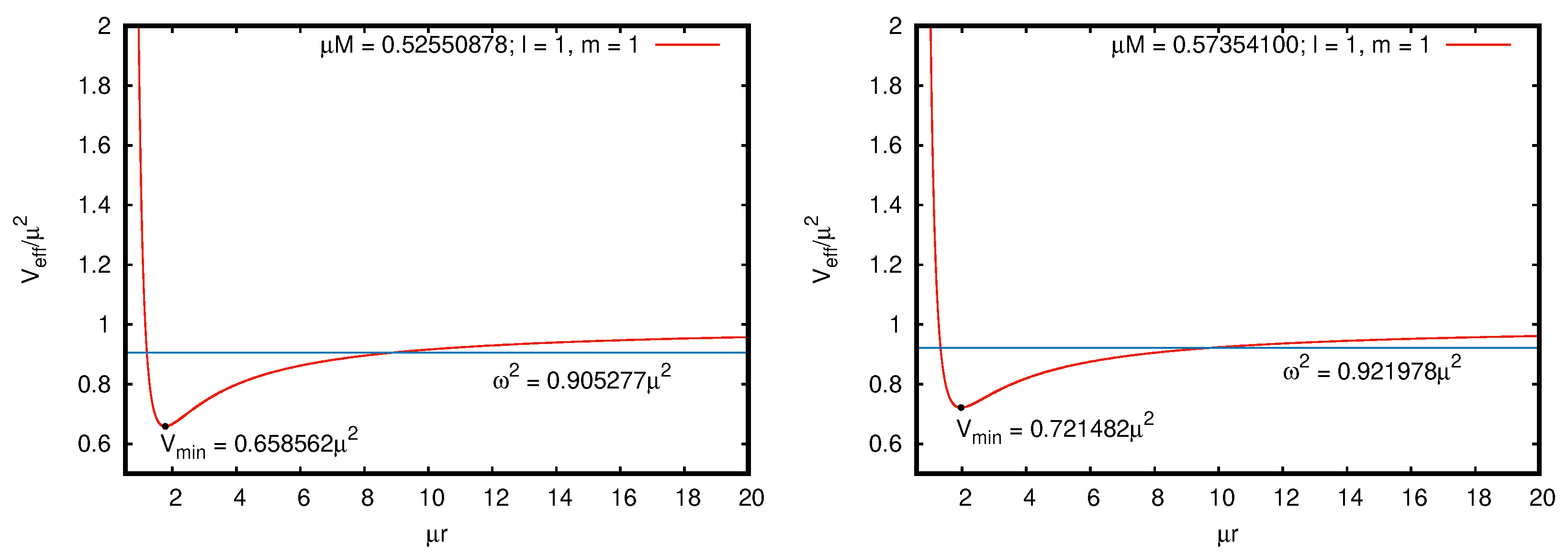
Figure 8.
Effective potential associated with a neutral scalar field () around an extremal Kerr black hole () (left panel). Effective potential associated with charged scalar clouds () coupled to an extremal Kerr–Newman black hole () (right panel). In both cases, and . The blue horizontal lines indicate the frequencies associated with boson cloud solutions.

Figure 9.
Solutions for the lapse N and the metric function A (evaluated at the equator ) for integers and , with and three values for .
Figure 9.
Solutions for the lapse N and the metric function A (evaluated at the equator ) for integers and , with and three values for .

Figure 10.
Solutions for the function B and the shift (evaluated at the equator ) for integers and , with and three different values for .
Figure 10.
Solutions for the function B and the shift (evaluated at the equator ) for integers and , with and three different values for .

Figure 11.
Amplitude of the scalar field with integers and (left panel) and (right panel), for a hairy black hole with and , respectively, for three different .
Figure 11.
Amplitude of the scalar field with integers and (left panel) and (right panel), for a hairy black hole with and , respectively, for three different .

Figure 12.
Amplitude of the scalar field associated with Figure 11 but depicted close to the horizon located at and , respectively.
Figure 12.
Amplitude of the scalar field associated with Figure 11 but depicted close to the horizon located at and , respectively.

Figure 13.
Amplitude of the scalar field for different values of and with and .

Figure 14.
Solutions for the lapse N and the metric function A (evaluated at the equator ) for integers and , with and three different values of .
Figure 14.
Solutions for the lapse N and the metric function A (evaluated at the equator ) for integers and , with and three different values of .

Figure 15.
Solutions for the function B and the shift (evaluated at the equator ) for integers and , with and three different values of .
Figure 15.
Solutions for the function B and the shift (evaluated at the equator ) for integers and , with and three different values of .

Figure 16.
Scalar field solutions associated with a hairy black hole with the event horizon located at and with integers (one node) and . The corresponding values for are displayed in the figure.
Figure 16.
Scalar field solutions associated with a hairy black hole with the event horizon located at and with integers (one node) and . The corresponding values for are displayed in the figure.

Figure 17.
Solutions for the lapse and the metric function for integers and , with and three different values of .
Figure 17.
Solutions for the lapse and the metric function for integers and , with and three different values of .

Figure 18.
Solutions for the function and the shift for integers and , with and three different values of .
Figure 18.
Solutions for the function and the shift for integers and , with and three different values of .

Figure 19.
Boson number (Noether charge) as a function of the angular frequency for two sequences of hairy black holes with horizons located at (left panel) and (right panel), respectively. For the first family of solutions, we have taken the azimuthal number , and for the second, . Both families correspond to the nodeless solutions ().

Figure 20.
Komar mass as a function of the BH angular frequency , taking , (left panel) and , (right panel). Both sequences correspond to hairy solutions with no nodes ().
Figure 20.
Komar mass as a function of the BH angular frequency , taking , (left panel) and , (right panel). Both sequences correspond to hairy solutions with no nodes ().

Figure 21.
Relative mass contributions and as a function of . In these plots, the event horizon is located at () (left panel) and () (right panel), respectively. Both panels correspond to scalar field solutions with .
Figure 21.
Relative mass contributions and as a function of . In these plots, the event horizon is located at () (left panel) and () (right panel), respectively. Both panels correspond to scalar field solutions with .

Figure 22.
Komar angular momentum as a function of taking , (left panel) and , (right panel). Both sequences correspond to scalar field solutions with .
Figure 22.
Komar angular momentum as a function of taking , (left panel) and , (right panel). Both sequences correspond to scalar field solutions with .

Disclaimer/Publisher’s Note: The statements, opinions and data contained in all publications are solely those of the individual author(s) and contributor(s) and not of MDPI and/or the editor(s). MDPI and/or the editor(s) disclaim responsibility for any injury to people or property resulting from any ideas, methods, instructions or products referred to in the content. |
© 2023 by the authors. Licensee MDPI, Basel, Switzerland. This article is an open access article distributed under the terms and conditions of the Creative Commons Attribution (CC BY) license (https://creativecommons.org/licenses/by/4.0/).
Share and Cite
MDPI and ACS Style
García, G.; Salgado, M.; Grandclément, P.; Gourgoulhon, E. From Scalar Clouds to Rotating Hairy Black Holes. Particles 2024, 7, 1-24. https://doi.org/10.3390/particles7010001
AMA Style
García G, Salgado M, Grandclément P, Gourgoulhon E. From Scalar Clouds to Rotating Hairy Black Holes. Particles. 2024; 7(1):1-24. https://doi.org/10.3390/particles7010001
Chicago/Turabian StyleGarcía, Gustavo, Marcelo Salgado, Philippe Grandclément, and Eric Gourgoulhon. 2024. "From Scalar Clouds to Rotating Hairy Black Holes" Particles 7, no. 1: 1-24. https://doi.org/10.3390/particles7010001