Finding Suitable Transect Spacing and Sampling Designs for Accurate Soil ECa Mapping from EM38-MK2

 ,
,  ,
,  and
and
Abstract
:1. Introduction
2. Materials and Methods
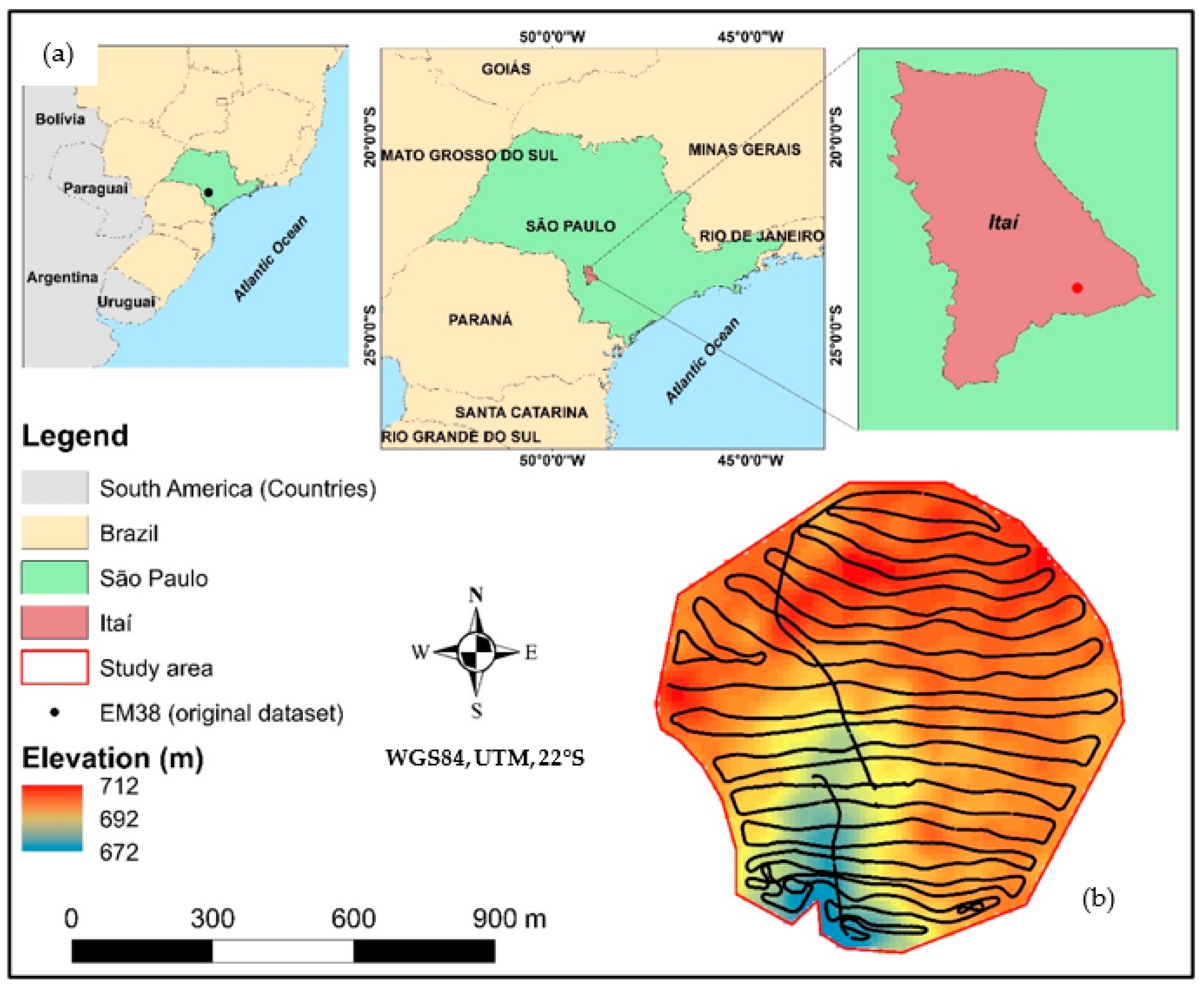
2.1. Study Area
2.2. EM38-MK2: Mobile Data Acquisition Structure and Survey Operation
2.3. EM38-MK2 Data Filtering and External Validation
2.4. Sampling Designs
2.4.1. Approach 1—Different Transect Spacings
2.4.2. Approach 2—Different Sample Densities Using Random and Douglas-Peucker Algorithm
2.5. Statistics, Interpolation, and Mapping Uncertainties
3. Results
3.1. Approach 1—Different Transect Spacings
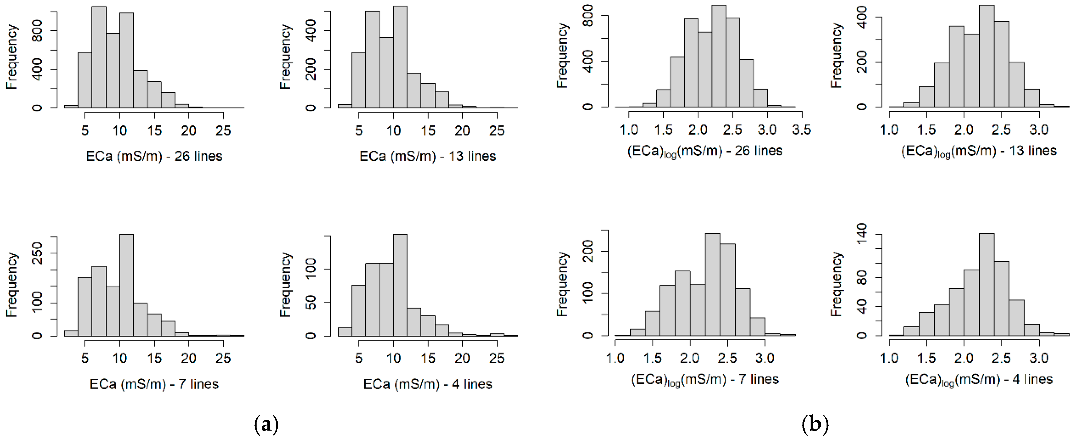
3.1.1. Exploratory Data Analysis
3.1.2. Fitting Semivariogram Models
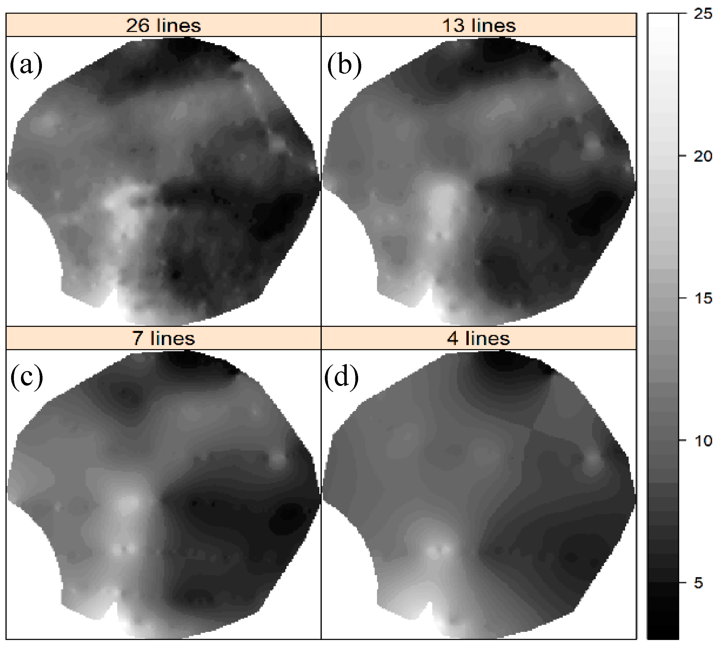
3.1.3. Mapping Soil ECa Spatial Variations
3.1.4. Map Uncertainty Assessment
3.2. Approach 2—Different Sample Densities
3.2.1. Exploratory Data Analysis
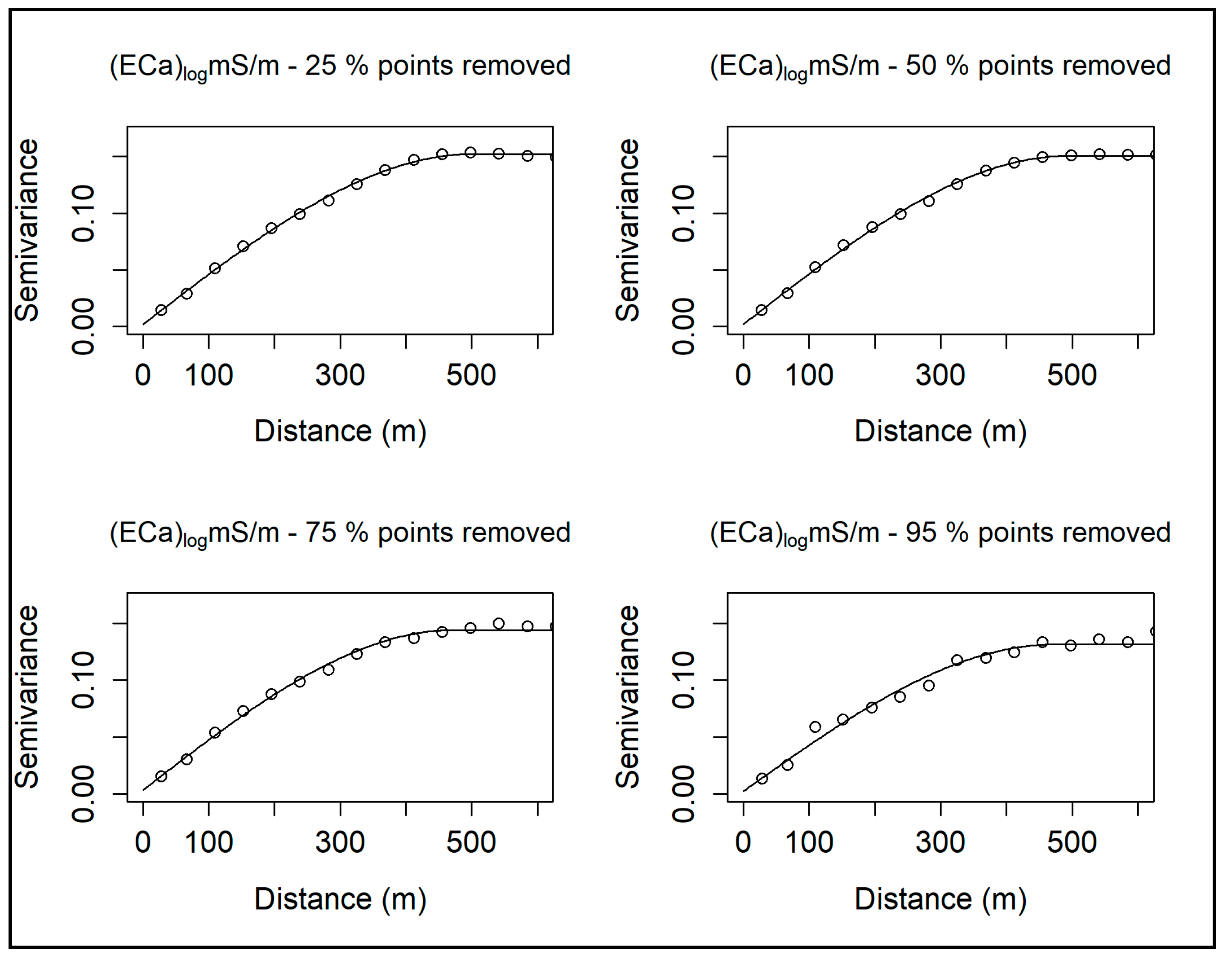
3.2.2. Fitting Semivariogram Models
3.2.3. Mapping Soil ECa Spatial Variations
3.2.4. Map Uncertainty Assessment
3.3. General Discussion
4. Conclusions
- Sampling designs for continuous PSS surveys are still lacking optimal operational standards, potentially compromising map uncertainty evaluations;
- Datasets from different transect spacings and sampling densities could preserve similar ranges in the magnitude of soil ECa mapping uncertainty variations;
- Accurate soil ECa maps were obtained from increasing transect spacing simulations up to 150 m; or decreasing sample densities to a maximum 75% and limiting the distance between observations to 180 m.
Author Contributions
Funding
Acknowledgments
Conflicts of Interest
References
- Larson, J.A.; Roberts, R.K.; English, B.C.; Cochran, R.L.; Wilson, B.S. A computer decision aid for the cotton yield monitor investment decision. Comput. Electron. Agric. 2005, 48, 216–234. [Google Scholar] [CrossRef]
- Benedetto, D.; De Castrignanò, A.; Diacono, M.; Rinaldi, M.; Ruggieri, S.; Tamborrino, R. Field partition by proximal and remote sensing data fusion. Biosyst. Eng. 2013, 114, 372–383. [Google Scholar] [CrossRef]
- Sudduth, K.A.; Drummond, S.T.; Kitchen, N.R. Accuracy issues in electromagnetic induction sensing of soil electrical conductivity for precision agriculture. Comput. Electron. Agric. 2001, 31, 239–264. [Google Scholar] [CrossRef]
- Hedley, C.B. The Development of Proximal Sensing Methods for Soil Mapping and Monitoring, and Their Application to Precision Irrigation. Ph.D. Thesis, Massey University, Palmerston North, New Zealand, 2009. [Google Scholar]
- de Gruijter, J.; Brus, D.; Bierkens, M.; Knotters, M. Sampling for Natural Resource Monitoring; Springer: Berlin/Heidelberg, Germany, 2006. [Google Scholar]
- O’Leary, G.J.; Grinter, V.; Mock, I. Optimal transect spacing for EM38 mapping for dryland agriculture in the Murray Mallee. In Proceedings of the 4th International Crop Science Congress, Brisbane, Australia, 26 September–1 October 2004. [Google Scholar]
- Scudiero, E.; Corwin, D.L.; Morari, F.; Anderson, R.G.; Skaggs, T.H. Spatial interpolation quality assessment for soil sensor transect datasets. Comput. Electron. Agric. 2016, 123, 74–79. [Google Scholar] [CrossRef]
- Sanches, G.M.; Magalhães, P.S.G.; Remacre, A.Z.; Franco, H.C.J. Potential of apparent soil electrical conductivity to describe the soil pH and improve lime application in a clayey soil. Soil Tillage Res. 2018, 175, 217–225. [Google Scholar] [CrossRef]
- Viscarra Rossel, R.A.; McBratney, A.B. Laboratory evaluation of a proximal sensing technique for simultaneous measurement of soil clay and water content. Geoderma 1998, 85, 19–39. [Google Scholar] [CrossRef]
- Sudduth, K.; Kitchen, N.; Myers, D.; Drummond, S. Mapping depth to argillic soil horizons using apparent electrical conductivity. J. Environ. Eng. Geophys. 2010, 15, 135–146. [Google Scholar] [CrossRef]
- Fulton, A.; Schwankl, L.; Lynn, K.; Lampinen, B.; Edstrom, J.; Prichard, T. Using EM and VERIS technology to assess land suitability for orchard and vineyard development. Irrig. Sci. 2011, 29, 497–512. [Google Scholar] [CrossRef] [Green Version]
- Viscarra Rossel, R.A.; Bouma, J. Soil sensing: A new paradigm for agriculture. Agric. Syst. 2016, 148, 71–74. [Google Scholar] [CrossRef]
- Adamchuk, V.; Ji, W.; Viscarra Rossel, R.; Gebbers, R.; Tremblay, N. Proximal soil and plant sensing. In Precision Agriculture Basics; Shannon, D.K., Clay, D.E., Kitchen, N.R., Eds.; John Wiley & Sons: Hoboken, NY, USA, 2018; pp. 119–140. [Google Scholar]
- Corwin, D.L.; Lesch, S.M. Apparent soil electrical conductivity measurements in agriculture. Comput. Electron. Agric. 2005, 46, 11–43. [Google Scholar] [CrossRef]
- USDA Soil Survey Manual; United States Department of Agriculture: Washington, DC, USA, 2017.
- McNeill, J.D. Electromagnetic Terrain Conductivity Measurement at Low Induction Numbers; Geonics Limited: Mississauga, ON, Canada, 1980. [Google Scholar]
- Vitharana, U.W.A.; Meirvenne, M.; Van Cockx, L.; Bourgeois, J. Identifying potential management zones in a layered soil using several sources of ancillary information. Soil Use Manag. 2006, 22, 405–413. [Google Scholar] [CrossRef]
- Rhoades, J.D.; Corwin, D.L. Determining soil electrical conductivity-depth relations using an inductive electromagnetic soil conductivity meter. Soil Sci. Soc. Am. J. 1981, 45, 255–260. [Google Scholar] [CrossRef]
- Lesch, S.M.; Rhoades, J.D.; Lund, L.J.; Corwin, D.L. Mapping soil salinity using calibrated electromagnetic measurements. Soil Sci. Soc. Am. J. 1992, 56, 540–548. [Google Scholar] [CrossRef]
- McKenzie, R.C.; Chomistek, W.; Clark, N.F. Conversion of electromagnetic inductance readings to saturated past extract values in soils for different temperature, texture, and moisture conditions. Can. J. Soil Sci. 1989, 69, 25–32. [Google Scholar] [CrossRef]
- Slavich, P.G. Determining ECa-depth profiles from electromagnetic induction measurements. Aust. J. Soil Res. 1990, 28, 443–452. [Google Scholar] [CrossRef]
- Huang, J.; Lark, R.M.; Robinson, D.A.; Lebron, I.; Keith, A.M.; Rawlins, B.; Tye, A.; Kuras, O.; Raines, M.; Triantafilis, J. Scope to predict soil properties at within-field scale from small samples using proximally sensed γ-ray spectrometer and EM induction data. Geoderma 2014, 232–234, 69–80. [Google Scholar] [CrossRef] [Green Version]
- Kachanoski, R.G.; Gregorich, E.G.; Van Wesenbeeck, I.J. Estimating spatial variations of soil water content using noncontacting electromagnetic inductive methods. Can. J. Soil Sci. 1988, 68, 715–722. [Google Scholar] [CrossRef]
- Sheets, K.R.; Hendrickx, J.M.H. Noninvasive soil water content measurement using electromagnetic induction. Water Res. Res. 1995, 31, 2401–2409. [Google Scholar] [CrossRef]
- Rodrigues, F.A.; Bramley, R.G.V.; Gobbett, D.L. Proximal soil sensing for precision agriculture: Simultaneous use of electromagnetic induction and gamma radiometrics in contrasting soils. Geoderma 2015, 243–244, 183–195. [Google Scholar] [CrossRef]
- Tavares, T.R.; Eitelwein, M.T.; Martello, M.; Trevisan, R.G.; Molin, J.P. Fusão de dados de condutividade elétrica e imagens Sentinel para caracterização da textura do solo. In Proceedings of the Congresso Brasileiro de Agricultura de Precisão, Curitiba, Paraná, Brazil, 2–4 October 2018. [Google Scholar]
- Triantafilis, J.; Santos, F.A.M. Resolving the spatial distribution of the true electrical conductivity with depth using EM38 and EM31 signal data and a laterally constrained inversion model. Aust. J. Soil Res. 2010, 48, 434–446. [Google Scholar] [CrossRef]
- Huang, J.; McBratney, A.B.; Minasny, B.; Triantafilis, J. 3D soil water nowcasting using electromagnetic conductivity imaging and the ensemble Kalman filter. J. Hydrol. 2017, 549, 62–78. [Google Scholar] [CrossRef]
- Cockx, L.; Van Meirvenne, M.; De Vos, B. Using the EM38DD soil sensor to delineate clay lenses in a sandy forest soil. Soil Sci. Soc. Am. J. 2007, 71, 1314–1322. [Google Scholar] [CrossRef]
- Heil, K.; Schmidhalter, U. The application of EM38: Determination of soil parameters, selection of soil sampling points and use in agriculture and archaeology. Sensors 2017, 17, 2540. [Google Scholar] [CrossRef] [Green Version]
- Machado, P.L.O.A.; Bernardi, A.C.C.; Valencia, L.I.O.; Molin, J.P.; Gimenez, L.M.; Silva, C.A.; Andrade, A.G.; Madari, B.E.; Meirelles, M.S.P. Mapeamento da condutividade elétrica e relação com a argila de Latossolo sob plantio direto. Pesquisa Agropecuária Brasileira 2006, 41, 1023–1031. [Google Scholar] [CrossRef] [Green Version]
- Becegato, V.A.; Ferreira, F.J.F. Gamaespectrometria, resistividade elétrica e susceptibilidade magnética de solos agrícolas no noroeste do estado do Paraná. Revista Brasileira Geofísica 2005, 23, 371–405. [Google Scholar] [CrossRef]
- Söderström, M.; Eriksson, J.; Isendahl, C.; Araújo, S.R.; Rebellato, L.; Pahl schaan, D.; Stenborg, P. Using proximal soil sensors and fuzzy classification for mapping Amazonian Dark Earths. Agric. Food Sci. 2013, 22, 380–389. [Google Scholar] [CrossRef]
- Sudduth, K.A.; Kitchen, N.R.; Wiebold, W.J.; Batchelor, W.D.; Bollero, G.A.; Bullock, D.G.; Clay, D.E.; Palm, H.L.; Pierce, F.J.; Schuler, R.T.; et al. Relating apparent electrical conductivity to soil properties across the north-central USA. Comput. Electron. Agric. 2005, 46, 263–283. [Google Scholar] [CrossRef]
- Islam, M.M.; Saey, T.; Meerschman, E.; De Smedt, P.; Meeuws, F.; Van De Vijver, E.; Van Meirvenne, M. Delineating water management zones in a paddy rice field using a floating soil sensing system. Agric. Water Manag. 2011, 102, 8–12. [Google Scholar] [CrossRef]
- Ramos, A.M.; Santos, L.A.R.; Fortes, L.T.G. Normais Climatológicas Do Brasil 1961–1990; Embrapa Arroz e Feijão (CNPAF): Brasília, Brazil, 2009. [Google Scholar]
- R Core Team. R: A language and environment for statistical computing. R Foundation for Statistical Computing, Vienna, Austria. Quant. Geogr. Basics 2019, 2, 250–286. [Google Scholar]
- Genolini, C. kmlShape: K-Means for Longitudinal Data Using Shape-Respecting Distance, R Package Version 0.9.5. 2016. Available online: https://CRAN.R-project.org/package=kmlShape (accessed on 18 May 2020).
- Wu, S.; Silva, A.C.G.; da Márquez, M.R.G. The Douglas-peucker algorithm: Sufficiency conditions for non-self-intersections. J. Braz. Comput. Soc. 2004, 9, 67–84. [Google Scholar] [CrossRef] [Green Version]
- Hengl, T. A Practical Guide to Geostatistical Mapping of Environmental Variables; Office for Official Publications of the European Communities: Luxembourg, 2007; p. 165. [Google Scholar]
- Lloyd, C.D.; Atkinson, P.M. Assessing uncertainty in estimates with ordinary and indicator kriging. Comput. Geosci. 2001, 27, 929–937. [Google Scholar] [CrossRef]
- Webster, R.; Oliver, M.A. Geostatistics for Environmental Scientists, 2nd ed.; John Wiley & Sons, Ltd.: Southern Gate, UK, 2007. [Google Scholar]
- Sun, W.; Whelan, B.; McBratney, A.B.; Minasny, B. An integrated framework for software to provide yield data cleaning and estimation of an opportunity index for site-specific crop management. Precis. Agric. 2013, 14, 376–391. [Google Scholar] [CrossRef]
- Han, S.; Hummel, J.W.; Georing, C.E.; Cahn, M.D. Cell size selection for site-specific crop management. Trans. ASAE 1994, 37, 19–26. [Google Scholar] [CrossRef]
- Pebesma, E.; Benedikt, G. Spatio-Temporal Interpolation using gstat. RFID J. 2020, 8, 204–218. [Google Scholar]
- Giebel, A.; Wndroth, O.; Reuter, H.I.; Kersebaum, K.-C.; Schawarz, J. How representatively can we sample soil mineral nitrogen? J. Plant Nutr. Soil Sci. 2006, 169, 52–59. [Google Scholar] [CrossRef]
- Triantafilis, J.; Lesch, S.M. Mapping clay content variation using electromagnetic induction techniques. Comput. Electron. Agric. 2005, 46, 203–237. [Google Scholar] [CrossRef]


| Varying Transect Spacing | ||
|---|---|---|
| Transect Spacing (m) | Number of Lines | Dataset Size |
| 40 | 26 | 3906 |
| 80 | 13 | 2119 |
| 150 | 7 | 1088 |
| 300 | 4 | 558 |
| Varying Sample Densities | ||
| Density reduction (%) | Random | Douglas-Peucker |
| Dataset size | ||
| 25 | 2930 | 2933 |
| 50 | 1953 | 1960 |
| 75 | 977 | 982 |
| 95 | 196 | 196 |
| Statistic | 26-Lines | 13-Lines | 7-Lines | 4-Lines | Validation Subset |
|---|---|---|---|---|---|
| Observations | 3906 | 2119 | 1088 | 559 | 400 |
| Minimum | 2.62 | 3.28 | 3.28 | 3.28 | 3.63 |
| Maximum | 26.25 | 26.25 | 26.25 | 26.25 | 25.31 |
| Mean | 9.58 | 9.63 | 9.72 | 9.68 | 9.62 |
| Median | 9.30 | 9.41 | 9.96 | 9.65 | 9.53 |
| Standard Deviation | 3.39 | 3.44 | 3.59 | 3.56 | 11.20 |
| Skewness | 0.68 | 0.73 | 0.65 | 0.95 | 3.35 |
| Kurtosis | 0.22 | 0.58 | 0.66 | 2.10 | 0.78 |
| Transect | Model | Nugget | Sill | Nugget/Sill (%) | Range (m) | MCD (m) |
|---|---|---|---|---|---|---|
| 26 | Spherical | 2.27 × 10⁻³ | 1.48 × 10⁻¹ | 1.51 | 505 | 186.57 |
| 13 | 2.76 × 10⁻³ | 1.50 × 10⁻¹ | 1.81 | 521 | 191.72 | |
| 7 | 2.39 × 10⁻³ | 1.62 × 10⁻¹ | 1.45 | 498 | 184.08 | |
| 4 | 7.00 × 10⁻³ | 1.30 × 10⁻¹ | 5.11 | 530 | 188.59 |
| Transect Lines | ME | RMSE |
|---|---|---|
| 26 | 0.00 | 0.54 |
| 13 | −0.11 | 0.67 |
| 7 | −0.13 | 0.94 |
| 4 | −0.25 | 1.73 |
| Statistics | 25% | 50% | 75% | 95% | ||||
|---|---|---|---|---|---|---|---|---|
| Random | DP | Random | DP | Random | DP | Random | DP | |
| Observations | 2930 | 2933 | 1953 | 1960 | 977 | 982 | 196 | 196 |
| Minimum | 2.62 | 3.44 | 3.48 | 3.48 | 3.48 | 3.48 | 3.48 | 3.48 |
| Maximum | 25.59 | 26.25 | 24.02 | 26.25 | 24.02 | 26.25 | 20.00 | 24.02 |
| Mean | 9.59 | 9.62 | 9.63 | 9.63 | 9.70 | 9.56 | 9.80 | 9.74 |
| Median | 9.30 | 9.26 | 9.34 | 9.26 | 9.41 | 9.06 | 9.59 | 9.47 |
| Std. Dev. | 3.41 | 3.42 | 3.44 | 3.47 | 3.43 | 3.52 | 3.29 | 3.56 |
| Skewness | 0.66 | 0,73 | 0.66 | 0.83 | 0.67 | 0.94 | 0.52 | 0.83 |
| Kurtosis | 0.12 | 0.34 | 0.06 | 0.62 | 0.13 | 1.04 | −0.43 | 0.69 |
| Density Reduction | Nugget | Sill | Nugget/Sill (%) | Range (m) | MCD | |||||
|---|---|---|---|---|---|---|---|---|---|---|
| Random | D-P | Random | D-P | Random | D-P | Random | D-P | Random | D-P | |
| 25% | 1.78 × 10⁻³ | 1.44 × 10⁻³ | 1.52 × 10⁻¹ | 1.47 × 10⁻¹ | 1.17 | 0.98 | 503 | 495 | 186.61 | 183.88 |
| 50% | 2.01 × 10⁻³ | 1.35 × 10⁻³ | 1.51 × 10⁻¹ | 1.48 × 10⁻¹ | 1.33 | 0.91 | 494 | 502 | 182.95 | 186.40 |
| 75% | 3.19 × 10⁻³ | 1.26 × 10⁻³ | 1.44 × 10⁻¹ | 1.46 × 10⁻¹ | 2.21 | 0.86 | 474 | 494 | 173.72 | 183.75 |
| 95% | 2.26 × 10⁻³ | 5.00 × 10⁻³ | 1.31 × 10⁻¹ | 1.52 × 10⁻¹ | 1.72 | 3.29 | 473 | 600 | 174.28 | 217.60 |
| Density Reduction (%) | Random | D-P | ||
|---|---|---|---|---|
| ME | RMSE | ME | RMSE | |
| 25 | −0.01 | 0.6 | 0.01 | 0.56 |
| 50 | 0 | 0.64 | 0 | 0.57 |
| 75 | −0.01 | 0.72 | −0.01 | 0.66 |
| 95 | −0.05 | 1.11 | −0.08 | 1.04 |
© 2020 by the authors. Licensee MDPI, Basel, Switzerland. This article is an open access article distributed under the terms and conditions of the Creative Commons Attribution (CC BY) license (http://creativecommons.org/licenses/by/4.0/).
Share and Cite
Rodrigues, H.M.; Vasques, G.M.; Oliveira, R.P.; Tavares, S.R.L.; Ceddia, M.B.; Hernani, L.C. Finding Suitable Transect Spacing and Sampling Designs for Accurate Soil ECa Mapping from EM38-MK2. Soil Syst. 2020, 4, 56. https://doi.org/10.3390/soilsystems4030056
Rodrigues HM, Vasques GM, Oliveira RP, Tavares SRL, Ceddia MB, Hernani LC. Finding Suitable Transect Spacing and Sampling Designs for Accurate Soil ECa Mapping from EM38-MK2. Soil Systems. 2020; 4(3):56. https://doi.org/10.3390/soilsystems4030056
Chicago/Turabian StyleRodrigues, Hugo M., Gustavo M. Vasques, Ronaldo P. Oliveira, Sílvio R. L. Tavares, Marcos B. Ceddia, and Luís C. Hernani. 2020. "Finding Suitable Transect Spacing and Sampling Designs for Accurate Soil ECa Mapping from EM38-MK2" Soil Systems 4, no. 3: 56. https://doi.org/10.3390/soilsystems4030056
APA StyleRodrigues, H. M., Vasques, G. M., Oliveira, R. P., Tavares, S. R. L., Ceddia, M. B., & Hernani, L. C. (2020). Finding Suitable Transect Spacing and Sampling Designs for Accurate Soil ECa Mapping from EM38-MK2. Soil Systems, 4(3), 56. https://doi.org/10.3390/soilsystems4030056