Abstract
This manuscript delves into the pivotal role of sustainable agriculture in addressing environmental challenges and meeting the nutritional demands of a burgeoning global population. The primary objective is to assess the impact of a recently developed eco-friendly fertilizer, denoted as SBO, which arises from the blend of organic and mineral components derived from agricultural waste, sulfur, and residual orange materials. These elements are bound together with bentonite. This study compares SBO with distinct fertilizer treatments, including horse manure (HM) and nitrogen–phosphorous–potassium (NPK), on two diverse tomato-growing soils, each characterized by unique chemical and biological properties. Furthermore, the research extends to evaluate the environmental implications of these fertilizers, with a specific focus on their carbon and water footprints. Soils have been chemically and biochemically analyzed, and carbon and water footprints (CF and WF, respectively) have been assessed. The results reveal substantial enhancements in soil quality with the application of SBO fertilizer. Both soils undergo a transition towards near-neutral pH levels, an increase in organic matter content, and heightened microbial biomass. SBO-treated soils exhibit notably superior enzyme activities. The Life Cycle Assessment (LCA) results affirm the sustainability of the SBO-based system, boasting the lowest CF, while NPK demonstrates the highest environmental impact. Consistently, the WF analysis aligns with these findings, indicating that SBO necessitates the least water for tomato production. In summary, this study underscores the critical importance of adopting sustainable fertilization practices for enhancing soil quality and reducing environmental footprints in agriculture. The promising results offer potential benefits for both food production and environmental conservation.
1. Introduction
Food systems currently account for approximately 33% of total human greenhouse gas (GHG) emissions, representing a significant and increasing share of global emissions [1]. The emissions from agricultural activities and land use, estimated at around 12.0 Gt CO2 per year, were quantified by the Food and Agriculture Organization (FAO) of the United Nations and the Intergovernmental Panel on Climate Change (IPCC) [1]. These emissions are expected to rise further due to the growing demand for food. One of the primary contributors to GHG emissions is the production of synthetic nitrogen (N) fertilizers used in crop cultivation. The application of these fertilizers is widely recognized as a major factor in the release of nitrous oxide (N2O) emissions from agricultural soils. N2O is a potent GHG, with a global warming potential 265 times greater than carbon dioxide (CO2) and methane (CH4) [2].
Moreover, in the early 1900s, a process was developed to mass-produce a compound containing ammonia, which greatly increased crop yields while utilizing less land. Ammonia is now one of the most extensively produced chemicals globally and is used in large quantities as a highly effective fertilizer [3]. However, excessive or improper application of nitrogen-based fertilizers can result in inefficient nitrogen uptake by plants, leading to an excess of nitrogen in the soil and subsequent N2O emissions. According to the IPCC, the global use of synthetic nitrogen fertilizers has increased by 800% since the 1960s. The FAO estimates that this quantity is projected to increase by an additional 50% by the year 2050 [1].
The European Union’s commitment to achieving a climate-neutral economy by 2050 is outlined in the European Green Deal, which emphasizes the role of every sector in this transition [4]. Soil, being a major carbon accumulator, stores twice as much carbon as the atmosphere and three times as much as terrestrial biomass [5]. Therefore, implementing appropriate and sustainable fertilization practices that enhance carbon storage and reduce CH4 and N2O emissions is crucial for agriculture to mitigate climate change while maintaining soil productivity [6].
Numerous researchers have demonstrated that long-term balanced fertilization, including sulfur (S) along with other macronutrients, can decrease N2O emissions without compromising productivity, highlighting the significant role of elemental sulfur in improving and maintaining soil fertility [7,8,9,10,11].
Sulfur is recognized as a vital element for promoting optimal soil health and enhancing the availability of essential nutrients such as nitrogen, phosphorus, and potassium to plant roots. It deserves re-evaluation and consideration as a key component of soil fertility and productivity. Factors such as intensive cultivation practices, the use of sulfur-free fertilizers, and a decline in atmospheric sulfur depositions have contributed to sulfur deficiency in agricultural soils [7,8]. Various studies have emphasized that sulfur deficiency leads to reduced nitrogen utilization from fertilizers and the production of crop proteins with significantly lower levels of sulfur-containing amino acids, particularly methionine, which greatly influences the nutritional value of plants [9,10,11].
Kulczycki et al. [12] provided evidence of the positive effects of elemental sulfur on plant yields and soil properties in crops such as mustard, wheat, rapeseed, and corn. Further investigations revealed a negative association between the application of elemental sulfur and microbial activities in soils, leading to a significant decrease in microbial biomass carbon (MBC) and enzyme activities [13].
This decline in microbial biomass and enzyme functions could potentially be attributed to a scarcity of carbon substrates, particularly in soils with low organic matter content. Conversely, numerous studies demonstrated the stimulating effects of organic amendments on soil microbial biomass and activities responsible for nutrient release [14,15]. These findings have prompted researchers to explore the combination of sulfur and organic matter. In this regard, Tabak et al. [16] discovered that incorporating waste sulfur with organic materials facilitated the simultaneous enrichment of soil with readily available sulfur and organic matter. Moreover, Holatko et al. [17] conducted research showing that the utilization of elemental sulfur in conjunction with organic material, such as digestate, enhanced the availability of sulfur, resulting in increased yields and improved crop quality. Additionally, this combination was found to enhance the activity of soil microbes [18]. Our previous works [19,20,21,22] demonstrated that fertilizers produced by reusing different kinds of biomasses were effective for land restoration and crop improvement.
Tomato represents 13.5% of the world’s vegetable production [23]. Several studies indicated that average GHG emissions for open-field tomato production were 0.2 and 2.0 kg CO2 eq kg tomato−1 [24]. Hillier et al. [25] calculated the carbon footprint (CF) variation of different food crop production and found that applied N-fertilizer contributed most to variability. Results in Lee et al. [26] research found that the field-scale variability of GHG emissions is controlled primarily by biochemical parameters rather than physical parameters. The results demonstrated that variations in microbial activity, influenced by tillage and irrigation practices, lead to distinct levels and combinations of field-scale controls on GHG emissions.
Aldaya and Hoekstra [27] analyzed Italian industrial tomato production that had a water footprint (WF) equal to 114 m3 t−1 (30% green, 50% blue, and 17% grey). Comparing these results with Chapagain and Orr [28], the blue component was in accordance with them, while green and grey were much higher in the Italian productive system due to different weather conditions and fertilizer inputs.
Simultaneous assessment of carbon and WF for agri-food products is desirable to provide better insights into key environmental issues than using either indicator in isolation [29]. These indicators measure the potential impact of a product throughout its entire life cycle in terms of GHG emissions and the consumption and degradation of water resources. The WF quantifies the volume of freshwater consumed or polluted (through evaporation or product incorporation) within a given time, while the CF indicates the Global Warming Potential over a defined period. The aim of this study was to evaluate the effects of agro-industrial waste-based fertilizer on the quality, CF, and WF of two soils used for growing industrial tomatoes (var. Big Rio F1), both in a climatic chamber and open field, compared to commonly used chemical and organic fertilizers.
2. Materials and Methods
2.1. Agro-Industrial Waste-Based Fertilizer Manufacturing
The fertilizer is composed of 85% elemental sulfur (S) pelletized with 10% bentonite clay (as the carrier and inert support) and 5% orange residue. After the pelletized phase, the mixtures were introduced in a rotary pastillator system, which deposits the liquid pads of the above-listed ingredients opportunely mixed on a heat exchanger in continuous steel tape for the solidification of the pods. In the end, pads with a diameter of 3/4 mm were obtained.
2.2. Soil Treatment
Fertilizers were tested on Tomato plants, variety Big Rio F1, grown in 30 cm diameter pots containing 9 kg of soil. For the trial, we conducted three replicates for each soil treatment. The experimentation took place in a climatic chamber to simulate the optimal environmental conditions for plant growth. The climatic conditions set in the climatic chamber for the germination phase were 25 °C, 70% humidity, and 800 Lux. For the vegetative development phase of the plants, climatic parameters were set following the climatic data from May until the end of August, considering that the vegetative cycle is 120 days for this variety. Two fertilizations were carried out: one at the beginning of the crop cycle and one at complete flowering. The fertilizer dosage to be used was chosen based on results obtained previously on various soils and different crops [19,20]. The fertilizer amount used for each treatment and pot is:
- (A)
- 1.2 g of synthetic fertilizer NPK (15-15-15) in which there are 0.18 g of N, 0.18 g of P2O5 and 0.18 g of K2O.
- (B)
- 13 g of organic fertilizer, in which there are 0.26 g of N, 0.26 g of P2O5, and 0.195 g of K2O. This fertilizer contains bovine, equine, sheep, and poultry manure mixed with litter, calcium sulfate, and olive pomace dust, which accounts for 50% of the total composition percentage.
- (C)
- 1.4 g of fertilizer sulfur–bentonite + orange residue.
2.3. Data Collection and Analysis
Soil samples were taken at 20 cm depth for each pot at the beginning of the trial, before planting the tomato seedling, and then six months later, after harvesting and subsequent removal of plants.
Data are expressed as means of three analyses for each treatment. Analysis of variance was carried out for all the data sets. One-way ANOVA with Tukey’s Honestly. Significant difference tests were carried out to analyze the effects of fertilizers on each of the various parameters measured; ANOVA and t-test were carried out using XLStat. Effects were significant at p ≤ 0.01. To explore. Relationships among different fertilizers on soil parameter datasets we analyzed using Principal Component Analysis (PCA) with XLStat.
2.4. Soil Physical, Chemical, and Biochemical Analysis before and after Treatment
Potted soils before treatment were analyzed for physical and chemical properties. Soils were taken in the Grecanica area (Table 1 and Table 2), specifically in the municipalities of Reggio di Calabria (RC) (soil 1) and Motta San Giovanni (RC) (soil 2). These soils were classified as sandy-loam soil (soil 1) and sandy-clay soil (soil 2) based on the FAO soil classification system [30]. Soil texture was assessed using the hydrometer method [31]. The pH was measured in distilled water (soil/solution ratio 1:2.5) with a glass electrode. Electric conductivity (EC) was determined in distilled water using a 1:5 soil/water suspension mechanically shaken at 15 rpm for 1 h and then detected with a Hanna instrument conductivity meter. Cation exchange capacity (CEC) was determined using the Mehlich methodology [32]. Organic carbon was assessed with the dichromate oxidation method [33] and transformed into organic matter by multiplying by 1.72; Total nitrogen (TN) was measured with the Kjeldahl method [34]. C/N was determined as a carbon/nitrogen ratio. Water-soluble phenols (WSPs) were extracted in triplicate, as reported by Kaminsky et al. [35]. Gallic acid was used as a standard, and the concentration of WSP compounds was expressed as Gallic Acid Equivalents (μg GAE g−1 d.s). MBC was determined using the chloroform fumigation-extraction procedure on fresh soil. [36] Fumigated and unfumigated soil sample extracts were used to detect soluble organic C using the methods of Walkley and Black [33].

Table 1.
Physical and chemical properties of soils before fertilization. Data are the means of three replicates ± standard deviation.
Table 2.
Soil enzymatic activities before fertilization. Dehydrogenase (DHA, µg INTF g−1 d.s h−1). Catalase activity (CAT O2/3 min/g d.s). Fluorescein diacetate hydrolase (FDA, µg fluorescein g−1 d.s). Urease (URE, N-NH4/g d.s/3 h). beta-glucosidase (ß-GLU, µg para-nitrophenol (p-NP) g/h). Protease (PRO µg Tyrosine g d.s 2 h). Data are the means of three replicates ± standard deviation.
Dehydrogenase (DHA) activity was detected with iodonitrotetrazolium chloride according to the von Mersi and Shinner method [37]. Catalase activity (CAT) was detected using the method of Kuush et al. [38], measuring the absorbance during the conversion of H2O2 to oxygen and water. The decrease in the absorbance was measured at 240 nm, utilizing the extinction coefficient of 39.4 M−1 cm−1. Fluorescein diacetate hydrolase (FDA) activity was determined according to the method of Adam and Duncan [39]. Beta-glucosidase activity was tested as reported by Valášková et al. [40] with the modifications reported in Muscolo et al. [19]. Soil (1 g fresh weight) was placed into a plastic tube and treated with 4 mL of modified universal buffer (MUB, pH 6). The reaction mixture contains 0.16 mL of 1.2 mM PNP substrate (p-nitrophenyl-β-D-glucoside) in 50 mM sodium acetate buffer (pH 5.0) and 0.04 mL of the sample. Reaction mixtures were incubated at 40 °C for 20–120 min. After incubation, the reaction was stopped, and the yellow color from the p-nitrophenol was developed by the addition of 0.1 mL of 0.5 M sodium carbonate; the p-nitrophenol absorbance was measured on a spectrophotometer at a wavelength of 400 nm and quantified by comparison with a standard curve. Protease activity was detected, as reported by Sidari et al. [41]. Two ml of phosphate buffer (0.1 M, pH 7.1) and 0.5 mL of 0.03 M N-a-benzoyl-L arginine amide (BAA) have been added to 1 g of wet soil. The mixture was incubated at 37 °C for 1 h and 30 min, then diluted to 10 mL with distilled water. The ammonium concentration was detected with an ammonium selective electrode (CRISON, micro-pH 2002). Urease activity was determined following the method of Kandeler and Gerber [42], with a few modifications, as reported in Sidari et al. [41]. Five grams of fresh soil were mixed with 2.5 mL of urea (80 mM) and 20 mL 0.1 M borate buffer at pH 10.0. After 2 h in an orbital shaker at 37 °C, 2.5 mL of urea were added to the control. 30 mL of KCl (2 M) were instead added to both the sample and, and shake for 30 min. One ml of the filtered solutions was mixed with 9 mL of distilled water, 5 mL of sodium/salicylate solution, and 2 mL of dichloroisocyanuric acid. Ammonium concentrations were determined at 690 nm by using a calibration curve. The results are reported as µg N-NH4/g d.s/3 h. [41].
2.5. Environmental Impact: Carbon and Water Footprint
The study was carried out in Grecanica Area, specifically in Motta San Giovanni, province of Reggio Calabria. The main features of the studied system were collected through visits to farms and direct interviews with farmers using a specific collection sheet. The farm carried out the treatments by subdividing four experimental plots, carrying out the treatments described in Section 2. The farm grew tomatoes of the Big Rio F1 variety, with a planting density of 3 plants/m2, with a sprinkler irrigation system. Insecticide treatment (with PRIMOR 500) and fungicide treatments (with DARAMUN) were the same for all experimental plots, as were soil tillage and harvesting. The only difference between the experimental plots was the fertilization. The farm inputs and outputs used in the analyzed systems are reported in Table 3.
Table 3.
Farm inputs and outputs used in the analyzed systems.
2.5.1. Carbon Footprint
The LCA approach, according to the ISO 14040:2006 [43], was used to estimate environmental impacts with a focus on Global Warming (GWP 100a) for the CF. This methodology contains four stages: goal and scope definition, life cycle inventory, life cycle impact assessment, and interpretation [44]. The system boundaries, as shown in Figure 1, start with the planting of tomato plants and end with harvesting. Following the PCR 2010:07, “Arable and vegetative crops” corresponds to CORE processes, which are the farming phases: transport of plants, acceptance of plants, planting, and harvest. In accordance with the PCR, [45] this study does not include manufacturing of buildings and capital goods other than agricultural machinery, business travel of personnel, travel to and from work by personnel, and research and development activities.
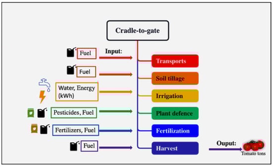
Figure 1.
System boundaries of CORE process of tomato production.
Furthermore, due to the lack of data, the analysis did not consider input transport (fertilizers and pesticides) from the place of production to the field. All the inputs used in the agricultural phase (fertilizers, pesticides, fuels, and various materials utilized during the harvesting) were considered. Primary data were collected in situ during the 2021–2022 agricultural year, from May to October, using a data collection sheet on a farm that carried out the experimentation in collaboration in the open field located in Motta San Giovanni (RC). The sample used for data collection is, therefore, homogeneous, consisting of a single farmer who divided his field into several experimental plots fertilized with different types of fertilizer (synthetic, organic, and sulfur bentonite orange waste-based fertilizer), the quantities of which are shown in Table 3 where all inputs and outputs (tons of tomato) of the production process are described. Direct emissions from fuel and lubricant were taken from SimaPro’s LCI database and calculated as reported by Pergola et al. [46].
Ammonia volatilization from mineral fertilizers application (namely NPK for system A) to soil incorporation, evaluated taking into account the type of mineral fertilizer and the geographical location of the olive system, was equal to 2% of the applied N-NH4. So, N2O emissions from fertilizers were computed considering the emission factor equal to 0.0125. Emission of synthetic pesticides to air, surface water, groundwater, and soil was estimated according to the methodology suggested by Hauschild [47]. These estimates considered both site conditions (soil organic matter, texture, climate, etc.) and physicochemical characteristics of the active ingredients (vapor pressure, half-life determined by photolysis, half-life in soil, adsorption coefficient to organic material in soil).
The impact assessment was performed using SimaPro 9.02, with the problem-oriented LCA method (CML-IA Baseline V3.06/EU25 + 3, 2000) developed by the Institute of Environmental Sciences of the University of Leiden [48]. The following impact categories were considered according to the selected method: abiotic depletion (AD); abiotic depletion (fossil fuels) (AD fossil fuels); global warming potential (GWP) or climate change; photochemical oxidation (PO); ozone layer depletion (ODP); human toxicity (HT); freshwater aquatic ecotoxicity (FWE); marine aquatic ecotoxicity (MAE); terrestrial ecotoxicity (TE); air acidification (AA) and eutrophication (EU).
2.5.2. Water Footprint
For this study, WF was performed as established by Hoekstra et al., 2011 [49] in “The Water Footprint Assessment Manual,” which defines the guidelines for the WF. The peculiarity of this methodology is the division of the WF into three components: blue, green, and grey. Blue, green, and grey components were calculated through the CROPWAT model. The total WF is given by the sum of components according to Equation (1):
WFtotal: WFgreen + WFBlue + WFgrey
For the WF green reported in Equation (3) and blue reported in Equation (4), the values for crop water requirement (CWR, m3 ha−1) are calculated using the formulas below:
WFgreen = CWUgreen/crop yield
WFblue = CWUblue/crop yield
The green and blue components of CWU (m3 ha−1) reported in Equations (4) and (5), respectively, were calculated by the accumulation of daily evapotranspiration (ET mm/day) over the whole growing season:
ETgreen represents green water evapotranspiration, and ETblue instead of blue water evapotranspiration [49]. The summation is performed over the period from the day of planting (day 1) to the day of harvest. The green and blue water evapotranspiration has been estimated using the CROPWAT model developed by the Food and Agriculture Organization of the United Nations [50], which is based on the method described by Allen et al. [51].
The CROPWAT model offers two different options to calculate evapotranspiration: the ‘crop water requirement option’ (assuming optimal conditions) and the ‘irrigation schedule option’ (including the possibility to specify actual irrigation supply in time [52] and for this study, we use the first option. According to Pellegrini et al. [53]:
- ETgreen was calculated as the minimum of Crop WaterRequirement (CWR, mm year−1) and effective precipitation (Peff, mm year−1).
- ETblue was estimated from Irrigation Requirement (IR) rates as the minimum between IR (m3 year−1) and the irrigation volume (Ieff, m3 ha−1 year−1). [53].
- IR was calculated as a constant value for the analyzed systems according to the following equation: IR = max (0; CWR-Peff).
In the CROPWAT 8.0 software, after entering the input data related to climate data of Reggio Calabria in the year 2021–2022, crop Kc, rainfall, and soil characteristics, we obtained the CWR needed to calculate the green and blue WF, as shown in Table 4.
Table 4.
Crop water requirement obtained from CROPWAT 8.0.
Following Hoekstra et al. 2011 [49], the grey component of WF was calculated as:
where:
WF product, grey = [(α × AR)/(Cmax − Cnat)]/Y
- AR is the chemical application rate to the field per hectare (kg ha−1);
- α is the leaching-run-off fraction;
- Cmax is the maximum acceptable concentration for the pollutant considered (kg m−3);
- Cnat is the natural concentration for the pollutant considered (kg m−3);
- Y is the crop yield (t ha−1).
For the grey component of the WF, only nitrogen fertilizers have been considered, according to Hoekstra et al., 2011 [49], because Nitrogen represents an important source of pollution in Europe, as can be seen from the Nitrates Directive 1990 [54]. The chemical application rate (AR) (kg ha−1) for the different cultivation systems used to calculate this footprint is reported in Table 3. From Legislative Decree 152/2006, the acceptable limit value for nitrogen was found to be 15 mg/L (Cmax), the maximum acceptable concentration (Cnat), following Hoekstra et al. [49] was considered to be 0, and a leaching factor (α) 0.1 was considered for all cultivation systems.
3. Results
3.1. Effect of Different Fertilizers on Soil Quality
The chemical properties of soil 1, assessed six months after the treatments, exhibited significant variations (Table 5). Notably, there were no significant changes in soil texture. However, in the soils treated with SBO, notable reductions were observed in both pH in water and KCl levels. Simultaneously, there was an increase in electrical conductivity (EC), suggesting the potential for an enhanced mineralization process with ion release. Additionally, the organic matter content, C/N ratio, CEC, and microbial biomass all experienced increases (Table 5).
Table 5.
Physical and chemical properties of soil 1 and soil 2 six months after the treatments with the different fertilizers: CTR = Control unfertilized soil; A = nitrogen–phosphorous–potassium; B = horse manure; C = sulfur bentonite + orange residue.
Conversely, in the soils treated with SBO, the phenol content and catalase activity decreased compared to all other treatments, while other enzyme activities increased. A strong positive and significant correlation was observed between MBC, organic matter, pH in KCl, C/N ratio, WSPs, FDA hydrolase, dehydrogenase protease, and urease activities. MBC correlated inversely with catalase activity and did not correlate with beta-glucosidase (Table 6).
Table 6.
Enzymatic activities of Soil 1 and Soil 2 six months after treatments with the different fertilizers. CTR = Control. soil without fertilizer; A = nitrogen:phosphorous:potassium; B = horse manure; C = sulfur bentonite + orange residue. Dehydrogenase (DHA, µg INTF g−1 d.s h−1), Catalase activity (CAT. O2/3 min/g d.s), Fluorescein diacetate hydrolase (FDA, µg fluorescein g −1 d.s), beta-glucosidase (ßGLU, µg para-nitrophenol (p-NP) g/h), Protease (PRO µg Tyrosine/g d.s/2 h), Urease (URE, N-NH4/g d.s/3 h).
Six months after the treatments, the chemical properties of soil 2 exhibited notable variations among the different treatment groups. However, in the soils treated with SBO, the reductions in both pH (measured in water) and KCl levels were particularly significant, surpassing the changes observed in soil 1. In contrast, EC, CEC, Organic Matter, C/N ratio, WSPs, and MBC all followed a similar increasing trend, as seen in soil 1 (Table 5).
When examining the biochemical data, akin to the findings in soil 1, the SBO-treated soil in soil 2 exhibited elevated levels of dehydrogenase fluorescein diacetate and beta-glucosidase activities, surpassing the other treatments, as previously observed. However, in the case of protease and urease activities, they displayed increases compared to control and NPK treatments, aligning with soil 1 (Table 6). Notably, they were found to be on par with the HM treatment, marking a departure from the results observed in soil 1.
Furthermore, catalase activity once again registered its lowest values in the SBO-treated soil, confirming the consistent pattern observed in soil 1.
The Pearson coefficient results for soil 1 indicated that all soil parameters were correlated with each other, albeit to varying degrees (Table 7). However, pH in H2O showed a significant positive correlation only with WSPs, Catalase, and Total Nitrogen.
Table 7.
Correlation matrix (Pearson (n)) of physical, chemical, and biochemical properties of soil 1 six months after treatments.
In contrast, soil 2 exhibited lower correlations among its variables (Table 8). pH showed a positive correlation only with Catalase, and no significant positive correlations were observed among the other soil variables, except for TOC, which correlated with WSP, MBC, DHA, PRO, and MBC, which correlated positively with TOC and with all soil enzymes except for CAT) and URE. PCA analysis confirmed the data of Pearson coefficient evidencing differences between the relations of the two soils with the analyzed soil properties (Figure 2 and Figure 3).
Table 8.
Correlation matrix (Pearson (n)) of physical, chemical, and biochemical properties of soil 2 six months after treatment.
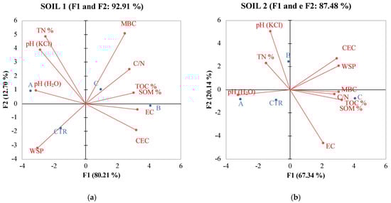
Figure 2.
PCA of physical and chemical properties of soil 1 (a) and soil 2 (b) six months after treatments with the different fertilizers with CTR = Control, soil without fertilizer; A = nitrogen:phosphorous:potassium; B = horse manure; C = sulfur bentonite + orange residue.
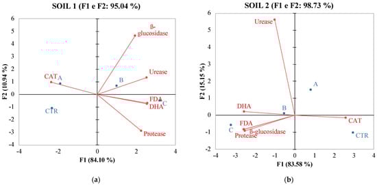
Figure 3.
PCA of enzymatic activities of soil 1 (a) and soil 2 (b) six months after treatments with the different fertilizers CTR = Control, soil without fertilizer; A = nitrogen–phosphorous–potassium; B = horse manure; C = sulfur bentonite + orange residue.
3.2. Environmental Impact
3.2.1. Carbon Footprint
The environmental analysis results, with a functional unit of 1 hectare and one ton of tomatoes considered for all impact categories, can be found in Table 9 and Table 10. For Global Warming Potential (GWP 100a), Figure 4 reveals that among the four analyzed systems, System A has the highest impact at 26.04 kg CO2 eq/t. This is followed by System B at 23.21 kg CO2 eq/t and System CTR at 23.05 kg CO2 eq/t. Notably, System C, which utilized Sulfur fertilizer bentonite, stands out as the most sustainable, with an impact value of 22.77 kg CO2 eq/t.
Table 9.
Environmental impacts per hectare of analyzed system CTR = Control, soil without fertilizer; A = nitrogen:phosphorous:potassium; B = horse manure; C = sulfur bentonite + orange residue.
Table 10.
Environmental impacts for a ton of tomatoes for each analyzed system: CTR = Control, soil without fertilizer; A = nitrogen–phosphorous–potassium; B = horse manure; C = sulfur bentonite + orange residue.
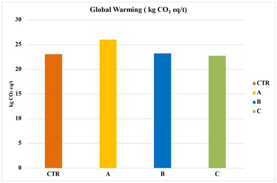
Figure 4.
Global warming of the entire life cycle in terms of kg of CO2 eq per ton of tomato. CTR = Control, soil without fertilizer; A = nitrogen:phosphorous:potassium; B = horse manure; C = sulfur bentonite + orange residue.
When broken down into individual phases, as seen in Figure 5, soil tillage emerges as the most impactful phase. This is followed by fertilization, registering an impact of 4.2 kg CO2 eq/t when applied. The organic fertilization using horse manure (System B) has an impact of 4.5 kg CO2 eq/t. Meanwhile, synthetic fertilization with NPK (System A) showcases the highest emissions among the systems, with values hitting 7.2 kg CO2 eq/t.
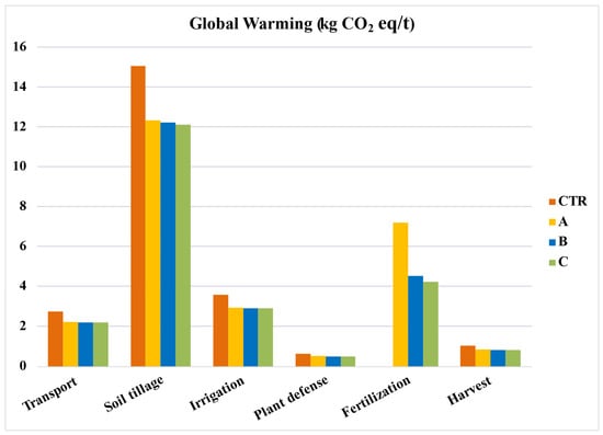
Figure 5.
Global warming per phase of the production process. Values per ton of tomato. CTR = Control, soil without fertilizer; A = nitrogen:phosphorous:potassium; B = horse manure; C = sulfur bentonite + orange residue.
3.2.2. Water Footprint
The results of the WF are presented by breaking it down into its components (green, blue, and grey) and then as total water consumption. Table 11 gives the data on yields, green evapotranspiration (Et green), blue evapotranspiration (Et blue), direct and indirect fraction of water used for the different systems analyzed, with the WF expressed in m3 per ton of tomato yield. Since all systems are located in Reggio Calabria (RC) and share identical climatic conditions (Table 4), green and blue evapotranspiration remains consistent across all systems, and differences in productivity result mainly from different fertilization approaches.
Table 11.
WF green and Blue of the analyzed systems. CTR = Control, soil without fertilizer; A = nitrogen:phosphorous:potassium; B = horse manure; C = sulfur bentonite + orange residue.
The system with the lowest WF is related to the use of sulfur-based bentonite fertilizers (A), which resulted in higher productivity. On the other hand, the control system (CTR) has the highest WF due to its lower production (Figure 6).
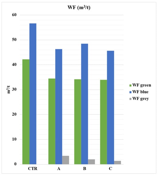
Figure 6.
Total Water Footprint (m3/t) broken down by its components (green, blue, grey) in the different cultivation systems. CTR = Control, soil without fertilizer; A = nitrogen–phosphorous–potassium; B = horse manure; C = sulfur bentonite + orange residue. Values are expressed in m3/t of tomato.
4. Discussion
4.1. Effect of Different Fertilizers on Soil Quality
In both soil 1 and soil 2, the results indicated significant alterations in soil properties due to the application of SBO fertilizer. These changes encompassed shifts in soil pH, reductions in KCl levels, increased EC, and notable enhancements in organic matter content, CEC, and microbial biomass.
The observed decrease in phenol content and catalase activity in SBO-treated soils compared to other treatments suggested that SBO may have an impact on soil microorganisms and their metabolic activities. This is further supported by the results of the Pearson coefficient showing a positive correlation between MBC organic matter, pH in KCl, C/N ratio, WSP, FDA hydrolysis, dehydrogenase protease activity, and urease activities. These findings underscore the complex relationship between soil properties and microbial responses to fertilizer treatments. Our data agree with the findings of Arunrat et al. [55], showing that over a 5-year period, the application of fertilizer and tillage practices significantly contributed to an augmentation in the diversity and richness of soil bacteria. Regarding bacterial abundance, it was strongly influenced by organic matter (OM) and organic carbon (OC).
In soil 2, similar trends were observed with SBO treatment, leading to notable changes in soil properties and enzyme activities. However, the correlation pattern between MBC and other factors differed from that in soil 1, as shown in the correlation matrix data, highlighting the influence of soil characteristics on the effects of added fertilizers.
Furthermore, the reduced Catalase activity in SBO-treated soils suggested that this fertilizer does not induce stressful conditions in these soils, supporting its suitability for soil health and productivity. “The intricate and diverse relationship between catalase activity and microbial biomass, in the two soils, is underscored, influenced by factors such as soil pH, organic matter content, and temperature”.
Principal Component Analysis (PCA) (Figure 2) results revealed multifaceted associations between SBO fertilizer and soil properties, both chemical and biochemical. These associations differed between soil 1 and soil 2, probably due to intrinsic dissimilarities in the soil conditions and microbial communities. Nonetheless, these findings provide valuable insights into the intricate interactions between fertilizers, soil characteristics, and microbial dynamics, which are essential for informed soil management practices and sustainable agriculture. Monitoring these parameters aids in assessing soil health, microbial activity, and nutrient cycling processes in differently-treated soil ecosystems, contributing to environmental management. The observed changes can positively affect tomato yield and quality. As already shown by Gao [56], tomato yield and quality were correlated to the amount of organic matter, which is known to play an important role in soil fertility and function. The trace elements in organic matter can meet the requirements of soil microorganisms, promote microbial activities, affect the soil–microorganism interaction, and consequently and indirectly influence tomato productivity. PCA analysis revealed, for soil 1, a positive correlation with SOM, MBC, TOC, and C/N ratio. This suggests a significant impact of SBO on soil chemical properties governing soil fertility. In contrast, for soil 2, an inverse correlation with these properties was observed. Turning to soil biochemical activity, in soil 1, the positioning in the II quadrant indicated an inverse correlation of SBO with fluorescein diacetate, dehydrogenase activity, and protease. This suggests a potential concentration threshold of SBO for this soil. Conversely, in soil 2, the positioning in the II quadrant revealed a positive correlation of SBO with FDA, protease, and beta-glucosidase.
Notably, HM and NPK did not show any significant relationship with the chemical and biochemical properties associated with soil fertility. In summary, these results underscore that SBO was the most effective fertilization strategy in both soils, and the variability in its effectiveness was linked to soil characteristics.
4.2. Environmental Impact
4.2.1. Carbon Footprint
The data offers a comparative understanding of the CF of various fertilization systems. System A’s substantial impact underscores the environmental concerns surrounding synthetic fertilizers like NPK.
The significant reduction in CF when using sulfur fertilizer bentonite (System C) indicates its potential as an environmentally friendly alternative. The distinctions between the systems and the high emissions linked to synthetic fertilization emphasize the necessity for transitioning towards more sustainable farming practices.
The evident emissions related to soil tillage and fertilization emphasize the environmental implications of these farming activities. Furthermore, the disparity in emissions between organic and synthetic fertilization methods warrants attention.
System B’s horse manure-based organic fertilization produces fewer emissions than the synthetic NPK method in System A, highlighting the environmental advantages of certain organic fertilizers. However, the fact that System C’s Sulfur fertilizer bentonite outperforms even the organic method suggests there are innovative solutions that can further reduce agriculture’s CF. Our results are in line with the findings of Wyngaard and Kissinger [57]. Theurl et al. [58], in a study comparing various tomato production systems in Austria, Spain, and Italy, showed that heating, packaging, and transport were the most important hot spots regarding GHG emissions associated with the different tomato supply chains and highlighted as the emissions from fertilizers, pesticides, soils, and infrastructures are relevant only in the case of intensive conventional production systems. Additionally, our results also agree with the findings of Toolkiattiwong et al. [59], indicating that more agricultural inputs, in terms of pesticides and fertilizers, augment the CFs and WFs and generate freshwater ecotoxicity.
4.2.2. Water Footprint
In the case of the cultivation system employing organic fertilizer (B), a higher impact is observed, mainly due to the direct fraction stemming from the water used in manure production. This indicates that organic fertilization may have implications for water use efficiency.
The results also revealed that the largest grey WF is associated with cultivation system A, which utilized synthetic NPK fertilizer. Conversely, due to the lower nitrogen content in sulfur bentonite fertilizer combined with orange residue, cultivation system C exhibits the lowest grey WF. This finding suggests that the choice of fertilizer can significantly impact the release of polluted water into the environment. Our results are in line with the findings of Evangelou et al. [60] and Wyngaard and Kissinger [57], who also showed how averages vary greatly depending on soil properties, local climatic conditions, and water management systems although no significant correlation the authors found with any individual soil property related to water retention. The high variability of WF values they found suggests the importance of considering water issues at the local scale level. As reported by Raluy et al. [61], WF results vary significantly within the same cultivars for the different local edaphoclimatic conditions and tree management models, as well as methodological choices adopted in the WF calculation.
When examining the Total WF, it becomes evident that the blue WF represents the largest percentage of WF when producing one ton of tomatoes for the various cultivation systems analyzed, followed by the green footprint. This highlights the importance of considering both surface and groundwater consumption in assessing the overall WF of agricultural practices.
While the grey WF constitutes only 1% of the total WF, it is a crucial indicator as it signifies the quantity of polluted water released into the environment. This underscores the need for sustainable fertilization practices to minimize environmental pollution.
Results evidenced that the impacts of the new fertilizer on the soil ecosystem varied in magnitude, consistently yielding positive effects on both soils. It can be confidently stated that the conversion of industrial and agricultural wastes into fertilizers holds the potential for economic and environmental benefits. These benefits arise from the reduced costs associated with waste disposal and the advantages to the soil resulting from a decrease in the use of mineral fertilizers, aligning with the principles and strategies of the circular economy. The results clearly demonstrated an enhancement in soil quality when utilizing sulfur-based pads, surpassing the performance of commonly employed organic and inorganic fertilizers. The continued reliance on the latter is discouraged in contemporary agriculture, particularly in the realm of organic farming.
In summary, the results emphasize the environmental benefits of System C, where tomato plants were fertilized with sulfur–bentonite combined with orange waste, as a more environmentally friendly choice in terms of WF. These findings contribute to the understanding of how fertilizer choices can influence water use efficiency and environmental impact in agriculture.
5. Conclusions
In summary, this fertilizer is environmentally friendly, and it plays a key role in fostering economic growth rooted in renewable resources. This responsible utilization of resources aligns seamlessly with the core tenets of a green economy, prioritizing the preservation and efficient use of resources. By minimizing its environmental footprint, this fertilizer actively contributes to the preservation of ecosystems and biodiversity—a cornerstone of a green economy. In doing so, it serves as a guardian of natural resources that form the bedrock of economic activities, particularly in agriculture. The sustainable production of this fertilizer has the potential to catalyze economic diversification by creating new markets and opportunities within the agricultural sector. This diversification can strengthen local economies, enhancing their resilience.
Author Contributions
Conceptualization, A.M. (Adele Muscolo), A.M. (Angela Maffia) and G.C.; methodology, G.C. and A.M. (Angela Maffia); software, A.M. (Angela Maffia); validation, A.M. (Adele Muscolo) and C.M.; formal analysis, F.M.; investigation, M.O.; data curation, F.C.; writing—original draft preparation, A.M. (Adele Muscolo); writing—review and editing, G.C.; visualization, A.M. (Adele Muscolo); supervision, G.C.; project administration, A.M. (Adele Muscolo); funding acquisition, A.M. (Adele Muscolo); All authors have read and agreed to the published version of the manuscript.
Funding
This research was funded by the Italian Ministry for University and Research (MUR), Project CN_00000022 “National Research Centre for Agricultural Technologies-Agritech”.
Institutional Review Board Statement
Not applicable.
Informed Consent Statement
Not applicable.
Data Availability Statement
The data presented in this study are available in section MDPI Research Data Policies at https://www.mdpi.com/ethics.
Acknowledgments
The authors express their gratitude to the Orfei Farm for providing both their land and personnel for the open field experiments.
Conflicts of Interest
The authors declare no conflict of interest.
References
- Rosenzweig, C.; Mbow, C.; Barioni, L.G.; Benton, T.G.; Herrero, M.; Krishnapillai, M.; Liwenga, E.T.; Pradhan, P.; Rivera-Ferre, M.G.; Sapkota, T.; et al. Climate change responses benefit from a global food system approach. Nat. Food. 2020, 1, 94–97. [Google Scholar] [CrossRef]
- Blandford, D.; Hassapoyannes, K. The Role of Agriculture in Global GHG Mitigation; Food, Agriculture and Fisheries Papers; OECD: Paris, France, 2018. [Google Scholar]
- Rouwenhorst, K.H.R.; Travis, A.S.; Lefferts, L. 1921–2021: A Century of Renewable Ammonia Synthesis. Sustain. Chem. 2022, 3, 149–171. [Google Scholar] [CrossRef]
- Wolf, S.; Teitge, J.; Mielke, J.; Schütze, F.; Jaeger, C. The European Green Deal—More Than Climate Neutrality. Intereconomics 2021, 56, 99–107. [Google Scholar] [CrossRef] [PubMed]
- Schlesinger, W.H.; Andrews, J.A. Soil respiration and the global carbon cycle. Biogeochemistry 2000, 48, 7–20. [Google Scholar] [CrossRef]
- Pan, S.Y.; He, K.H.; Lin, K.T.; Fan, C.; Chang, C.T. Addressing nitrogenous gases from croplands toward low-emission agriculture. NPJ Clim. Atmos. Sci. 2022, 5, 43. [Google Scholar] [CrossRef]
- Hinckley, E.L.S.; Crawford, J.T.; Fakhraei, H.; Driscoll, C.T. A shift in sulfur-cycle manipulation from atmospheric emissions to agricultural additions. Nat. Geosci. 2020, 13, 597–604. [Google Scholar] [CrossRef]
- Haneklaus, S.; Bloem, E.; Schnug, E. History of Sulfur Deficiency in Crops. Sulfur A Missing Link between Soils Crops Nutr. 2008, 50, 45–58. [Google Scholar]
- Głowacka, A.; Gruszecki, T.; Szostak, B.; Michałek, S. The response of common bean to sulphur and molybdenum fertilization. Int. J. Agron. 2019, 3830712. [Google Scholar] [CrossRef]
- Głowacka, A.; Jariene, E.; Flis-Olszewska, E.; KiełtykaDadasiewicz, A. The Effect of Nitrogen and Sulphur Application on Soybean Productivity Traits in Temperate Climates Conditions. Agronomy 2023, 13, 780. [Google Scholar] [CrossRef]
- Pandurangan, S.; Sandercock, M.; Beyaert, R.; Conn, K.L.; Hou, A.; Marsolais, F. Differential response to sulfur nutrition of two common bean genotypes differing in storage protein composition. Front. Plant Sci. 2015, 6, 92. [Google Scholar] [CrossRef]
- Kulczycki, G. The Effect of Elemental Sulfur Fertilization on Plant Yields and Soil Properties. In Advances in Agronomy; Academic Press: Cambridge, MA, USA, 2021; ISBN 0065-2113. [Google Scholar]
- Malik, K.M.; Khan, K.S.; Billah, M.; Akhtar, M.S.; Rukh, S.; Alam, S.; Munir, A.; Mahmood Aulakh, A.; Rahim, M.; Qaisrani, M.M.; et al. Organic Amendments and Elemental Sulfur Stimulate Microbial Biomass and Sulfur Oxidation in Alkaline Subtropical Soils. Agronomy 2021, 11, 2514. [Google Scholar] [CrossRef]
- Liang, Q.; Chen, H.; Gong, Y.; Yang, H.; Fan, M.; Kuzyakov, Y. Effects of 15 years of manureand mineral fertilizers on enzyme activities in particle-size fractions in a North China Plain soil. Eur. J. Soil Biol. 2014, 60, 112–119. [Google Scholar] [CrossRef]
- Zhongqi, H.E.; Pagliari, P.H.; Waldrip, H.M. Applied and environmental chemistry of animal manure: A review. Pedosphere 2016, 26, 779–816. [Google Scholar]
- Tabak, M.; Lisowska, A.; Filipek-Mazur, B. Bioavailability of Sulfur from Waste Obtained during Biogas Desulfurization and the Effect of Sulfur on Soil Acidity and Biological Activity. Processes 2020, 8, 863. [Google Scholar] [CrossRef]
- Holatko, J.; Brtnicky, M.; Mustafa, A.; Kintl, A.; Skarpa, P.; Ryant, P.; Baltazar, T.; Malicek, O.; Latal, O.; Hammerschmiedt, T. Effect of Digestate Modified with Amendments on Soil Health andPlant Biomass under Varying Experimental Durations. Materials 2023, 16, 1027. [Google Scholar] [CrossRef] [PubMed]
- Heinze, S.; Hemkemeyer, M.; Schwalb, S.A.; Khan, K.S.; Joergensen, R.G.; Wichern, F. Microbial Biomass Sulphur—An Important Yet Understudied Pool in Soil. Agronomy 2021, 11, 1606. [Google Scholar] [CrossRef]
- Muscolo, A.; Mallamaci, C.; Settineri, G.; Calamarà, G. Increasing soil and crop productivity by using agricultural wastes pelletized with elemental sulfur and bentonite. Agron. J. 2007, 109, 1900–1910. [Google Scholar] [CrossRef]
- Muscolo, A.; Romeo, F.; Marra, F.; Mallamaci, C. Transforming agricultural, municipal and industrial pollutant wastes into fertilizers for a sustainable healthy food production. J. Environ. Manag. 2021, 17, 113771. [Google Scholar]
- Panuccio, M.R.; Attinà, E.; Basile, C.; Muscolo, A. Use of Recalcitrant Agriculture Wastes to Produce Biogas and Feasible Biofertilizer. Waste Biomass Val. 2016, 7, 267–280. [Google Scholar] [CrossRef]
- Panuccio, M.R.; Papalia, T.; Attinà, E.; Giuffrè, A.; Muscolo, A. Use of digestate as an alternative to mineral fertilizer: Effects on growth and crop quality. Arch. Agron. Soil Sci. 2019, 65, 700–711. [Google Scholar] [CrossRef]
- FAO: Food and Agriculture Organization of the United Nations. Available online: https://www.fao.org (accessed on 6 June 2023).
- Pishgar-Komleh, S.H.; Akram, A.; Keyhani, A.; Raei, M.; Elshout, P.M.F.; Huijbregts, M.A.J.; van Zelm, R. Variability in the carbon footprint of open-field tomato production in Iran—A case study of Alborz and East-Azerbaijan provinces. J. Clean. Prod. 2017, 142, 1510–1517. [Google Scholar] [CrossRef]
- Hillier, K.; Hawes, C.; Squire, G.; Hilton, A.; Wale, S.; Smith, P. Carbon footprints of food crop production. Int. J. Agric. Sustain. 2009, 7, 107–118. [Google Scholar] [CrossRef]
- Lee, J.; Six, J.; King, A.P.; Kessel, C.V.; Rolston, E.D. Tillage and feld scale controls on greenhouse gas emissions. J. Environ. Qual. 2006, 35, 714–725. [Google Scholar] [CrossRef] [PubMed]
- Aldaya, M.M.; Hoekstra, A.Y. The water needed for Italians to eat pasta and pizza. Agric. Syst. 2010, 103, 351–360. [Google Scholar] [CrossRef]
- Chapagain, A.K.; Orr, S. An improved water footprint methodology linking global consumption to local water resources: A case of Spanish tomatoes. J. Environ. Manag. 2009, 90, 1219–1228. [Google Scholar] [CrossRef] [PubMed]
- Page, G.; Ridoutt, B.; Bellotti, B. Carbon and water footprint tradeoffs in fresh tomato production. J. Clean. Prod. 2012, 32, 219–222. [Google Scholar] [CrossRef]
- FAO. Methods of Analysis for Soils of Arid and Semi-Arid Regions; Food and Agricultural Organization: Rome, Italy, 2007; p. 57. [Google Scholar]
- Bouyoucos, G.J. Hydrometer method improved for making particle size analysis of soils. Agron. J. 1962, 54, 464–465. [Google Scholar] [CrossRef]
- Mehlich, A. Rapid Determination of Cation and Anion Exchange Properties and pHe of Soils. J. Assoc. Off. Agric. Chem. 1953, 36, 445–457. [Google Scholar] [CrossRef][Green Version]
- Walkley A, Black IA An examination of the Degtjareff method for determining soil organic matter and a proposed modification of the chromic acid titration method. Soil Sci. 1934, 37, 29–38. [CrossRef]
- Kjeldahl, J. Neue Methode zur Bestimmung des Stickstoff in organishen Kopern. Anal. Chem 1883, 22, 354–358. [Google Scholar]
- Kaminsky, R.; Muller, W.H. The extraction of soil phytotoxins using neutral EDTA solution. Soil Sci. 1977, 124, 205–210. [Google Scholar] [CrossRef]
- Vance, E.D.; Brookes, P.C.; Jenkinson, D.S. An extraction method for measuring soil microbial biomass C. Soil Biol. Biochem. 1987, 19, 703–707. [Google Scholar] [CrossRef]
- Von Mersi, W.; Schinner, F. An improved and accurate method for determining the dehydrogenase activity of soils with iodonitrotetrazolium chloride. Biol. Fertil. Soils 1991, 11, 216–220. [Google Scholar] [CrossRef]
- Kuush, H.; Bjorklund, M.; Rystrion, L. Purification and characterization of a novel bromoperoxidase-catalase isolated from bacteria found in recycle pulp white water. Enzym. Microb. Technol. 2001, 28, 617–624. [Google Scholar]
- Adam, G.; Duncan, H. Development of a sensitive and rapid method for the measurement of total microbial activity using fluorescein diacetate (FDA) in a range of soils. Soil Biol. Biochem. 2001, 33, 943–951. [Google Scholar] [CrossRef]
- Valášková, V.; Šnajdr, J.; Bittner, B.; Cajtham, T.; Merhautová, V.; Hofrichter, M.; Baldrian, P. Production of lignocellulose-degrading enzymes and degradation of leaf litter by saprotrophic basidiomycetes isolated from a Quercus petraea forest. Soil Biol. Biochem. 2007, 39, 2651–2660. [Google Scholar] [CrossRef]
- Sidari, M.; Ronzello, G.; Vecchio, G.; Muscolo, A. Influence of slope aspects on soil chemical and biochemical properties in a Pinus laricio forest ecosystem of Aspromonte (Southern Italy). Eur. J. Soil Biol. 2008, 44, 364–372. [Google Scholar] [CrossRef]
- Kandeler, E.; Gerber, H. Short-term assay of soil urease activity using colorimetric determination of ammonium. Biol. Fert. Soils 1988, 6, 68–72. [Google Scholar] [CrossRef]
- UNI EN ISO 14044:2006; Environmental Management, Life Cycle Assessment—Requirements and Guidelines. International Organization for Standardization (ISO): Geneva, Switzerland, 2006.
- Maffia, A.; Palese, A.M.; Pergola, M.; Altieri, G.; Celano, G. The Olive-Oil Chain of SalernoProvince (Southern Italy): A LifeCycle Sustainability Framework. Horticulturae 2022, 8, 1054. [Google Scholar] [CrossRef]
- PCR- Product Category Rules. Arable and Vegetable Crops un CPC 011, 012, 014, 017, 0191. Version 1.0.1 Valid ultil: 7 December 2024. Available online: https://environdec.com/pcr-library/with-documents (accessed on 10 April 2023).
- Pergola, M.; Persiani, A.; Pastore, V.; Palese, A.M.; Arous, A.; Celano, G. A comprehensive Life Cycle Assessment (LCA) of three apricot orchard systems located in Metapontino area (Southern Italy). J. Clean. Prod. 2017, 142, 4059–4071. [Google Scholar] [CrossRef]
- Hauschild, M.Z. Estimating pesticide emissions for LCA of agricultural products. In Agricultural Data for Life Cycle Assessments; Weidema, B.P., Meeusen, M.J.G., Eds.; LCA Net Food: The Hague, The Netherlands, 2000; Volume 2, pp. 64–79. [Google Scholar]
- CML; Bureau, B.G. Life Cycle Assessment: An Operational Guide to the ISO Standards; School of SystemEngineering, Policy Analysis and Management, Delft University of Technology: Delft, The Netherlands, 2001. [Google Scholar]
- Hoekstra, A.Y.; Chapagain, A.K.; Mekonnen, M.M. The Water Footprint Assessment Manual: Setting the Global Standard; Earthscan: London, UK, 2011. [Google Scholar]
- FAO. Database CROPWAT. 2010. Available online: https://www.fao.org/land-water/databases-and-software/cropwat/en/ (accessed on 9 October 2023).
- Allen, R.G.; Pereira, L.S.; Raes, D.; Smith, M. Crop Evapotranspiration: Guidelines for Computing Crop Water Requirements; FAO Irrigation and Drainage Paper No. 56; FAO: Rome, Italy, 1998. [Google Scholar]
- Xin, D.; Wang, S.; Chen, B. The Blue, Green and Grey Water consumption for crop Production in Heilongjiang. Energy Procedia 2019, 158, 3908–3914. [Google Scholar]
- Pellegrini, G.; Ingrao, C.; Camposeo, S.; Tricase, C.; Contó, F.; Huisingh, D. Application of water footprint to olive growing systems in the Apulia region: A comparative assessment. J. Clean. Prod. 2016, 112, 2407–2418. [Google Scholar] [CrossRef]
- European Council. Directive n 91/676/EEC of 12 December 1991 Concerning the Protection of Waters against Pollution Caused by Nitrates from Agricultural Sources. Available online: https://eur-lex.europa.eu/LexUriServ/LexUriServ.do?uri=CELEX%3A31991L0676%3AEN%3AHTML (accessed on 9 October 2023).
- Arunrat N, Sansupa C, Sereenonchai S and Hatano R Stability of soil bacteria in undisturbed soil and continuous maize cultivation in Northern Thailand. Front. Microbiol. 2023, 14, 1285445. [CrossRef]
- Gao, F.; Li, H.; Mu, X.; Gao, H.; Zhang, Y.; Li, R.; Cao, K.; Ye, L. Effects of Organic Fertilizer Application on Tomato Yield and Quality: A Meta-Analysis. Appl. Sci. 2023, 13, 2184. [Google Scholar] [CrossRef]
- Wyngaard, S.R.; Kissinger, M. Tomatoes from the desert: Environmental footprints and sustainability potential in a changing world. Front. Sustain. Food Syst. 2022, 6, 994920. [Google Scholar] [CrossRef]
- Theurl, M.C.; Haberl, H.; Erb, K.H.; Lindenthal, T. Contrasted greenhouse gas emissions from local versus long-range tomato production. Agron. Sustain. Dev. 2014, 34, 593–602. [Google Scholar] [CrossRef]
- Toolkiattiwong, P.; Arunrat, N.; Sereenonchai, S. Environmental, Human and Ecotoxicological Impacts of Different Rice Cultivation Systems in Northern Thailand. Int. J. Environ. Res. Public Health 2023, 20, 2738. [Google Scholar] [CrossRef]
- Evangelou, E.; Tsadilas, C.; Tserlikakis, N.; Tsitouras, A.; Kyritsis, A. Water Footprint of Industrial Tomato Cultivations in the Pinios River Basin: Soil Properties Interactions. Water 2016, 8, 515. [Google Scholar] [CrossRef]
- Raluy, R.G.; Quinteiro, P.; Dias, A.C. Water Footprint of Forest and Orchard Trees: A Review. Water 2022, 14, 2709. [Google Scholar] [CrossRef]


Disclaimer/Publisher’s Note: The statements, opinions and data contained in all publications are solely those of the individual author(s) and contributor(s) and not of MDPI and/or the editor(s). MDPI and/or the editor(s) disclaim responsibility for any injury to people or property resulting from any ideas, methods, instructions or products referred to in the content. |
© 2023 by the authors. Licensee MDPI, Basel, Switzerland. This article is an open access article distributed under the terms and conditions of the Creative Commons Attribution (CC BY) license (https://creativecommons.org/licenses/by/4.0/).