The Loss of Soil Parent Material: Detecting and Measuring the Erosion of Saprolite

Abstract

Soil parent material is a fundamental natural resource for the generation of new soils. Through weathering processes, soil parent materials provide many of the basic building blocks for soils and have a significant bearing on the physico-chemical makeup of the soil profile. Parent materials are critical for governing the stock, quality, and functionality of the soil they form. Most research on soil parent materials to date has aimed to establish and measure the processes by which soil is generated from them. Comparatively little work has been performed to assess the rates at which soil parent materials erode if they are exposed at the land surface. This is despite the threat that the erosion of soil parent materials poses to the process of soil formation and the loss of the essential ecosystem services those soils would have provided. A salient but unanswered question is whether the erosion of soil parent materials, when exposed at the land surface, outpaces the rates at which soils form from them. This study represents one of the first to detect and measure the loss of soil parent material. We applied Uncrewed Aerial Vehicle Structure-From-Motion (UAV-SfM) photogrammetry to detect, map, and quantify the erosion rates of an exposed saprolitic (i.e., weathered bedrock) surface on an agricultural hillslope in Brazil. We then utilized a global inventory of soil formation to compare these erosion rates with the rates at which soils form in equivalent lithologies and climatic contexts. We found that the measured saprolite erosion rates were between 14 and 3766 times faster than those of soil formation in similar climatic and lithological conditions. While these findings demonstrate that saprolite erosion can inhibit soil formation, our observations of above-ground vegetation on the exposed saprolitic surface suggests that weathered bedrock has the potential to sustain some biomass production even in the absence of traditional soils. This opens up a new avenue of enquiry within soil science: to what extent can saprolite and, by extension, soil parent materials deliver soil ecosystem services?

1. Introduction

Soil erosion represents a pervasive challenge [1]. The thinning of soil profiles poses a long-term threat to the delivery of ecosystem services such as crop production, water filtration, carbon sequestration, nutrient cycling, and the provision of habitats and raw materials [2]. The decline or loss of these services results in cascading impacts on the sustainability of environments, societies, and economies.

Without mitigation, the thinning of soil profiles can lead to the exposure of the underlying soil parent material [3]. For soils overlying consolidated lithologies, the soil parent material comprises bedrock. The uppermost zone of bedrock (i.e., immediately below the soil profile) is referred to here as the ‘saprolite’. This represents the zone of bedrock that is most chemically weathered, but retains some of the structure and fabric of the rock, and is the parent material from which residual soils are formed [4,5]. Extending downwards from the saprolite is a continuum of increasingly less weathered bedrock. As a soil parent material, saprolite is a fundamental resource, providing the basic building blocks for soils, and one which can govern the stock, quality, and functionality of the soils it forms.

Most of the work on saprolite has focused on the process of soil formation. For example, research has been carried out to demonstrate how chemical weathering dissolves the primary minerals contained within saprolite, thereby weakening its resistance to subsequent weathering [4]. Others have measured the rates at which saprolite is converted into soil, and explored the factors that may affect this process [6,7]. However, if saprolite is exposed at the land surface, it becomes susceptible to erosion. This represents a key, albeit understudied, threat to the generation of new soil, and thus a cascading issue for the species, communities, and systems that rely on the delivery of soil ecosystem services.

The rates of saprolite erosion at the land surface have not been thoroughly studied [8]. However, some work has been undertaken to identify the erosion mechanisms. For example, Lidmar-Bergstrom showed how saprolite could become etched or stripped from an exposed surface of fresh bedrock, and suggested this was due to glacial erosion or a similar mass movement process [9]. Other work has considered how bedrock exposed at the surface is less susceptible to erosion than saprolite that is overlain by soil, because precipitation often runs off exposed rock surfaces, reducing the contact time between the water and rock and, in consequence, limiting weathering processes [10]. Elsewhere, research has explored how this erodibility is governed, in part, by the mineralogical, compositional, and textural properties of saprolite [11,12]. Some researchers have deployed aggregate stability tests to assess saprolite erodibility [11] while others have used drop-cone penetrometer measurements [12]. More recent work within critical zone science has developed advanced imaging techniques, such as electrical resistivity tomography, to observe how saprolite thickness changes due to erosion [13].

Our scarce knowledge of the rates at which saprolite erodes undermines our ability to preserve it effectively so that these parent materials are afforded opportunities to develop soil profiles. Where soil erosion has led to the exposure of the underlying saprolite, saprolite erodibility is an important factor for assessing future erosion risk as well as considering effective solutions for habitat restoration. One of the current barriers is the lack of an accurate method by which to detect, observe, and measure saprolite erosion. Although many soil erosion models are widely established, such as RUSLE, these have not been tested and adapted for saprolitic surfaces [14,15,16,17]. In addition to the limitations related to model uncertainties, and the availability of input data, these models are also unable to determine and partition different forms of erosion (e.g., sheet, rill, inter-rill) [16,17]. Instead, empirical erosion plots can be used to determine both the rates and general forms of erosion, although these can only determine the total sediment loss and are less able to detect any mid-slope colluviation that may occur [18].

A promising alternative to the use of erosion models and erosion plots is Uncrewed Aerial Vehicle Structure from Motion (UAV-SfM) photogrammetry, which presents a low-cost and high-resolution option for the detection, mapping, and measurement of surface erosion and colluviation [19,20]. UAV-SfM photogrammetry is a methodology whereby a series of digital elevation models (DEMs) are generated using aerial imagery captured during UAV flights. These DEMs are sequentially assembled, with the differences in elevation over distinct time intervals indicating landscape alterations such as denudation (e.g., soil erosion) or accretion (e.g., soil deposition). Differential DEMs, or DEMs of Difference (DoDs), are then used to quantify gross soil displacement volumes within specific temporal frames. One of the significant advantages of utilizing UAVs for image capture is their capability to generate extensive spatial coverage within relatively brief durations. This attribute is particularly beneficial for the high-frequency assessment of geomorphic phenomena. Pertinent to this study, UAVs provide a viable means of quantifying erosion in steep or otherwise inaccessible catchments, where conventional empirical methods are hindered by challenging topography or terrain instability.

In this paper, we deploy UAV-SfM photogrammetry to detect, map, and quantify the rates of saprolite erosion at the field scale. We then compare these rates of saprolite erosion with data on soil formation from similar climatic contexts and lithologies to assess the severity of the impact that these saprolite losses have on the initial development of soil profiles.

2. Materials and Methods

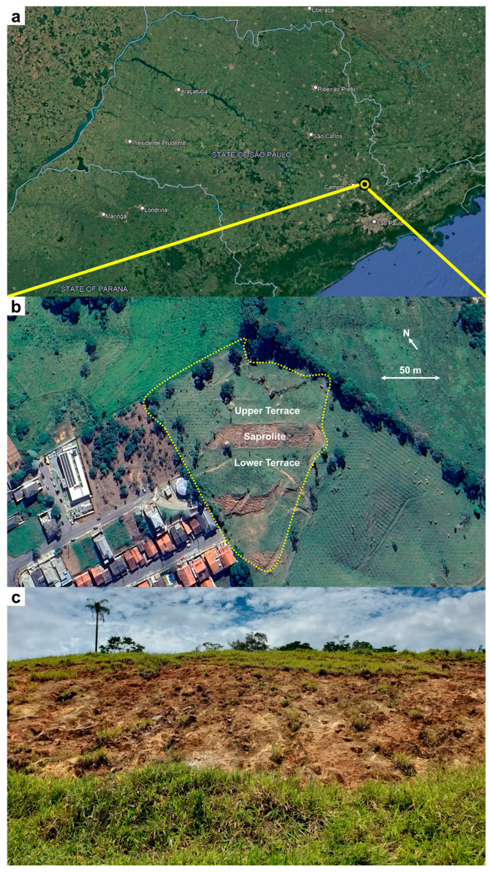
2.1. Study Location

This investigation was conducted down a southeast-facing hillslope situated northeast of Morungaba, São Paulo, Brazil (22°52′27.40″ S, 46°47′7.60″ W) (Figure 1a). The experimental area sits in a humid subtropical climate (i.e., Cfa on the Koppen Classification) [21]. It is characterized by a mean annual temperature of 20 °C, with the warmest month occurring in January, where the average maximum temperature can reach 31.4 °C, and the coolest in July, where the average minimum temperature is 7 °C. The mean annual rainfall is 1614 mm, with January being the wettest month (245.6 mm) and the driest being July (22.7 mm). Moreover, the study site is located 700 m from the Morungaba-SP Automated Weather Station, from which precipitation and temperature data were collected over the duration of the investigation (17 March–22 July 2021). These data are presented in Table S1.

A reconnaissance survey was conducted at the site in February 2021 to undertake a classification of the soil and underlying lithology. This reconnaissance mission showed that the soils across the site had originally developed from gneissic and migmatitic (i.e., metamorphic) rocks. Our area of interest (6600 m²) can be divided into three compartments (Figure 1b): an upper terrace (~2500 m²), a ramp or escarpment (~1400 m²), and a lower terrace (~2700 m²). The upper and lower terraces are nearly flat surfaces, whereas the ramp has a slope gradient ranging from 32 to 43%.

Prospective auger borings revealed that the soils on both the lower and upper terraces are seldom deeper than 1 m and are mostly friable saprolite mixed with soil. For the purposes of this study, saprolite is delineated from soil by being chemically weathered yet structurally consolidated bedrock; in other words, saprolite retains some of the structure and fabric of the bedrock, whereas soil particles are unconsolidated (i.e., granular or aggregated). Both terraces are covered by grass (Figure 1c). The material on the ramp is a moderately cohesive, eluviated saprolite, classified as paralytic material, saprock, or schistearap/granearap [22]. Importantly, this saprolite is exposed at the land surface, and has been since circa 2004 when a sizable (yet unquantified) volume of soil was removed from this area for use in a nearby construction project. The presence of classic erosion features on this exposed saprolite suggests that the ramp is actively eroding and depositing material at its toe. The escarpment displays proto-rills and rill development; there is scarce vegetation (mostly only pioneer communities), commensurate with an actively eroding surface; and, immediately below the escarpment, colluvial deposits are observable, formed from sediments that have eroded upslope.

Another legacy of the localized soil excavation in c. 2004 is the exposure of three landscape remnants. Remnant 1 is in the western portion of the ramp (Figure 2), remnant 2 is in the northern portion of the upper terrace, and remnant 3 lies 30 m east from the lower terrace. The upper surfaces of the remnants, elevated between 1.5 and 2.5 m from the surrounding land surface, are vegetated with grasses and shrubs, and showcase well-preserved original soil profiles. Field and laboratory characterization of these three soil profiles identified two Chromic Abruptic Lixisols (Clayic, Ochric) at remnants 1 and 2, and a Dystric Chromic Cambisol (Loamic, Ochric) at remnant 3, according to the World Reference Base soil classification [23]. The Lixisols have a 0.3 m sandy clay loam A horizon, with a weak fine to very fine subangular blocky structure, overlying a 0.9 m clayey argic B horizon, with a moderate medium to fine subangular blocky structure. Saprolite (Cr horizon) is present at 1.1 m. The Cambisol present in remnant 3 has a 0.15 m clay loam A horizon, and a 0.65 m clay loam cambic B horizon on top of a loam BC horizon, with the latter extending beyond the depth of 2.0 m.

2.2. Sampling and Analyzing Soil and Saprolite

To characterize and compare the properties of the soil on the upper and lower terraces with those of the exposed saprolite on the ramp, a second field sampling survey was conducted. A straight-line transect, parallel to the slope, was established on both the upper and lower terraces. Given the focus on saprolite in this investigation, this transect bifurcated into two (west and east) transects in the saprolite zone (i.e., between Plot A and Plot B, and between Plot B and Plot C) (Figure 3a).

Samples of the soil and saprolite surface were extracted manually from these transects using a hand auger to a depth of 20 cm. Undisturbed samples were collected in 100 cm³ volumetric cylinders to determine bulk density, total porosity, macroporosity, and microporosity. Physical and chemical analyses of these samples were carried out at the Soils and Environmental Resources Centre of the Agronomic Institute (IAC), Brazil.

Bulk density was analyzed using the core method [24]. Particle density was analyzed using the pycnometer method with 96% ethyl alcohol [25]. Total porosity was calculated as the ratio between bulk density and particle density. Microporosity was estimated as the water content retained by soil at the tension of 6 kPa, whereas macroporosity was calculated as the difference between total porosity and microporosity. Organic carbon was determined by the oxidation of carbon with potassium dichromate in an acid medium, followed by the determination of the remaining Cr⁶⁺ by colorimetry [26]. Determination of soil pH was carried out in a 0.01 mol/L CaCl₂ solution; exchangeable P, K, Ca, and Mg by the ion exchange resin method; exchangeable Al by 1 mol/L KCl; and potential acidity (H + Al) by the SMP buffer solution. Cation exchange capacity was the sum of exchangeable Ca, Mg, K, Na, Al, and H. Total elements were determined by microwave-assisted digestion with nitric and hydrochloric acid (EPA 3051A method) followed by ICP-AES (EPA 6010D method), according to EPA SW-846 except for K, which was determined by flame photometry after digestion by the EPA 3051A method [27].

Saturated hydraulic conductivity (K_sat) was determined using a Guelph permeameter, which was inserted to a depth of 20 cm. Three repeat measurements were conducted for each sampling point. K_sat (mm.h⁻¹) was determined according to Equation (1) [28]:

$$K_{sat}=\frac{CQ}{\left[2\pi H^2+C\pi a^2+\left(\frac{2\pi }{a}\right)\right]}\ast \mathrm{36,000}$$

(1)

where C is a dimensionless proportionality constant; Q is the constant flow (cm³ s⁻¹); a is the radius of the permeameter (cm); H is the constant load applied (cm); and α is the correction parameter of the porous medium (cm s⁻¹).

The constant flow (Q) and parameter C were determined according to Equations (2) and (3) [28]:

𝑄 = 𝐴𝑅

(2)

where Q is the constant flow (cm³ s⁻¹); A is the reservoir area of the permeameter (cm²); and R is the water level drop ratio (cm s⁻¹).

𝐶 = 𝐴(𝐻𝑎)𝐵

(3)

where A and B are soil-texture-dependent constants.

2.3. UAV-SfM Experimental Set-Up and Flights

2.3.1. Image Acquisition

A DJI Phantom 4 RTK UAV was used for aerial image acquisition. The UAV features an integrated gimbal-stabilized FC6310R camera with a 1” CMOS 20-megapixel (5472 × 3648) sensor, 84° field of view (FOV), and 24 mm focal length. The lens aperture was set to f/5.6 and images were acquired in JPG format.

Six flights were performed in the study area from March 2021 to June 2021. The flights were conducted automatically using a combination of orthogonal and oblique photos to provide convergent image geometries between the lines [29]. In order to reduce the influence of direct sunlight at noon, flights were conducted either in the morning or in the afternoon on cloudy days. Flight heights were over 15 m with a nominal ground sampling distance of 4.1 mm. A total of 110 photos were taken in each survey, with 75% of forward and side overlap.

For georeferencing, 38 ground control points (GCPs) were installed around the area (Figure 3a), with 28 points used for control and 10 as check points to estimate the precision and the accuracy of the 3D models by calculating the root mean square error (RMSE). The coordinates of the points were established by the total station (Geodetic GD2i, accuracy 2 mm) within an arbitrary local coordinate system.

2.3.2. SfM Point Cloud Generation

The generation of three-dimensional point clouds was performed using SfM photogrammetry, which enables the reconstruction of the topography from randomly distributed and oriented images captured using uncalibrated cameras [30,31,32]. The images were processed using the co-alignment technique [33] in the SfM software Agisoft Metashape Professional^® v1.7. The photogrammetric processing settings applied in Metashape are listed in

Table 1. Metashape parameter settings used during the point cloud generation.

Alignment/Reconstruction	Parameter	Setting
Point cloud alignment parameters	Accuracy	Highest
	Generic preselection	Yes
	Reference preselection	Yes
	Key point limit	120,000
	Tie point limit	0
	Filter point by mask	No
Dense point cloud reconstruction parameters	Quality	Medium
	Depth filtering	Mild

.

The co-alignment process, an advancement in the UAV-SfM methodology, enables the construction of multi-temporal 3D models by processing imagery from multiple surveys collectively during the alignment phase. This technique diverges from traditional UAV-SfM approaches that generate 3D models from each survey independently. Co-alignment has demonstrated significant improvements in the accuracy of topographic change detection by reducing relative errors between digital surface models (DSMs) without necessitating GCP [33,34,35]. Furthermore, research [36,37] has shown the efficacy of co-alignment with varying imagery sources, including UAV, terrestrial, and satellite, under different conditions, and its potential for automation in generating accurate models. Saponaro et al. highlighted its robustness in point cloud comparison for change detection [38]. Collectively, these studies affirm the effectiveness of co-alignment for enhancing both the relative and absolute accuracies within SfM applications.

Following this innovative co-alignment workflow, photographic data from multiple surveys were integrated into a unified dataset within Metashape. This process enabled the execution of point detection, matching, initial bundle adjustment, and optimization with uniform parameters. Distinct camera calibration groups were designated for each survey to manage variations in calibration parameters. The methodology leveraged similarities in imagery across surveys to identify key points and generate common tie points, enhancing the alignment. After completing the alignment and optimization, the dataset was divided into subsets for each survey, maintaining the integrity of sparse point clouds, positional data, and calibration details. Dense point clouds were calculated for each survey period, leveraging the comprehensive data integration facilitated by co-alignment.

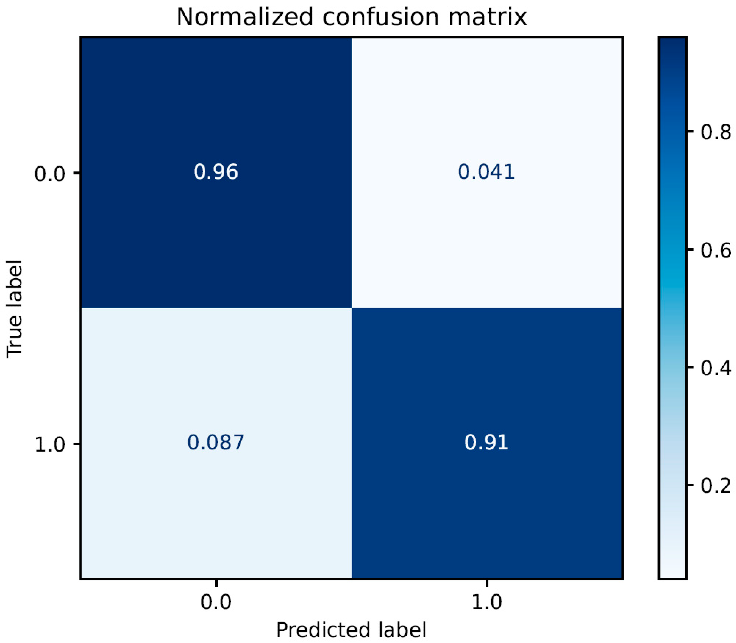
2.3.3. Classification of Vegetation in SfM Point Cloud

To facilitate the removal of vegetation from the point clouds and to enable the measurement of soil erosion and deposition, a methodical procedure was implemented within the workflow for the classification of vegetation in an SfM point cloud via a Random Forest algorithm. Initially, labeled points were generated by identifying vegetation over different time periods, resulting in approximately 75,000 vegetation points and 140,000 ground points. The Random Forest model was trained using different configurations, specifically with 10, 100, and 300 trees, wherein the model with 300 trees yielded the most accurate results (Figure 4). The training and test split comprised 70% and 30% of the data, respectively. Subsequent to the initial training, an iterative selection process was employed to identify features of the greatest importance, which led to an observed increase in the model’s accuracy (Figure 5). The most effective feature selection was then applied in practical scenarios.

Training the Random Forest model involved varying sets of parameters calculated for different search radii, including 0.015, 0.03, 0.5, 0.1, 0.15, and 0.2. The parameters considered in this context encompass roughness, first-order moment, mean curvature, number of neighbors, the sum of eigenvalues, planarity, linearity, sphericity, and the RGB color components, along with a composite parameter. This comprehensive approach ensured a robust and accurate vegetation classification within the SfM point cloud.

2.3.4. Erosion Measurements Using SfM Photogrammetry

The filtered dense point clouds were exported into Surfer 16 software, converted to raster DEMs of a 4 mm grid size using the nearest-neighbor interpolation method, and cropped to remove the plot edges. The erosion calculations were performed using Simpson’s rule [39], which assumes nonlinearity in the profile between grid points. This technique shows greater precision for determining volume than linear methods, such as the trapezoidal rule [40]. Erosion rates, calculated in terms of volume, were recalculated into volume per square meter using the plot area, as measured using SfM photogrammetry.

3. Results

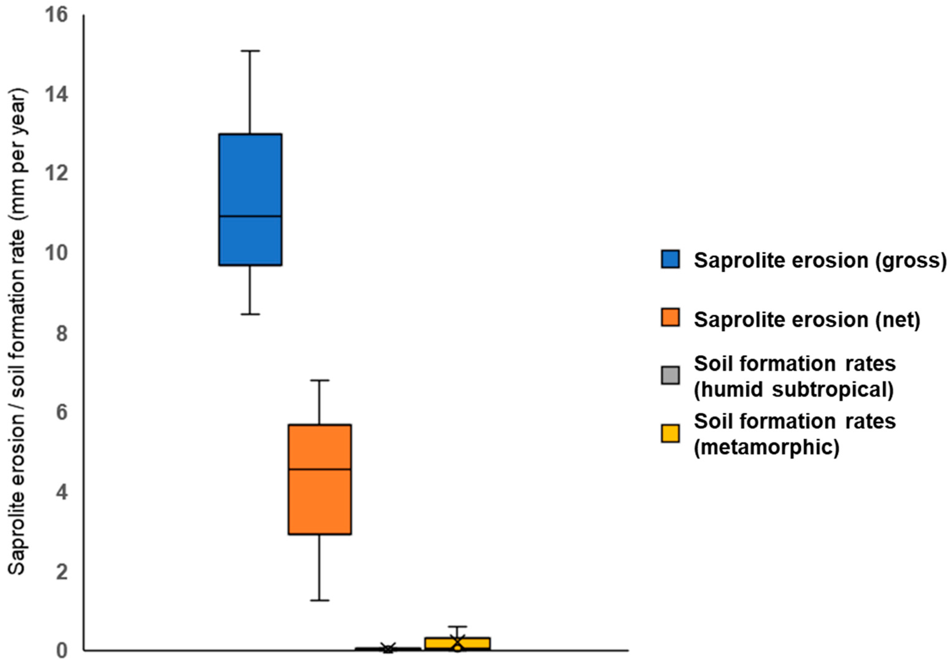
3.1. Rates of Saprolite Erosion

Table 2. Erosion and deposition of saprolite across the three saprolite observation plots throughout the experimental period.

	Erosion (−ve) or Deposition (+ve) of Saprolite (cm3 m2)
	Plot A	Plot B	Plot C
17 March–1 April	+0.10	+0.08	−0.06
1 April–30 April	+0.18	+0.28	+0.31
30 April–26 May	−0.15	−0.26	−0.07
26 May–17 June	−0.21	−0.25	−0.18
17 June–22 July	−0.11	−0.14	−0.05
Total erosion over the observation period	0.05	0.65	0.37
Total deposition over the observation period	0.27	0.36	0.31
Net erosion over the observation period	0.20	0.29	0.05

shows the material lost and gained across the three saprolite plots throughout the experimental period. Net erosion occurred across all saprolite plots, although the magnitude of this loss differed between them, with the largest net erosion occurring in Plot B (0.29 cm³/m²) and the smallest in Plot C (0.05 cm³/m²). The range of net erosion is mostly explained by the large range of gross erosion rates (0.29 cm³/m²) rather than for those of deposition (range: 0.08 cm³/m²). The gross erosion observed in Plot B was nearly 1.8× the magnitude of that measured in Plot C. Moreover, saprolite erosion in Plot B was more than five times the size of that seen in Plot C.

Although a net loss of saprolite was observed in all plots, the first 1.5 months of the experimental period showed a phase of net material gain (Table 2). Predominantly, the source of this material gain was soil transported from the upper terrace and subsequently deposited on the saprolite ramp. Plots A, B, and C received 0.27 cm³/m², 0.36 cm³/m², and 0.31 cm³/m² of soil from the upper terrace throughout this period, respectively. Plot C experienced a phase of net material loss during the first 24 days, but this was followed by a net material gain of 0.32 cm³/m² throughout the subsequent month. From 1 May through to the conclusion of the observation period (22 July), all three plots were subject to net erosion. For Plots A and C, the most erosive period was between 26 May and 17 June, whilst for Plot B, the period of greatest erosion was between 30 April and 26 May. The period over which the least erosion was observed for all plots was the final observation period between 17 June and 22 July.

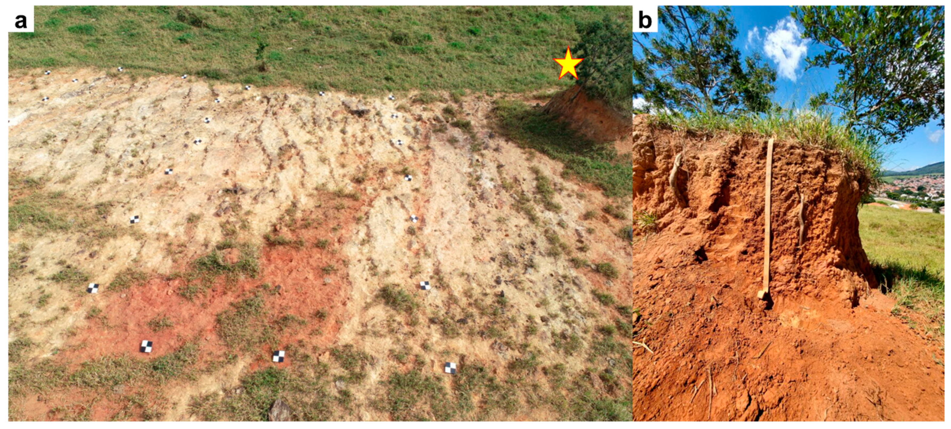
3.2. Characterization of Soil and Saprolite

Table 3. Physical and chemical properties of the soils and saprolite extracted from the study site.

	Units	UT-1	UT-2	UT-3	LT-1	LT-2	LT-3	SAP-E1	SAP-E2	SAP-E3	SAP-E4	SAP-W1	SAP-W2	SAP-W3	SAP-W4	Median Soil	Median Saprolite
Particle density	g/cm3	2.70	2.65	2.58	2.62	2.68	2.69	2.67	2.62	2.69	2.61	2.61	2.63	2.62	2.61	2.67	2.62
Total porosity	m3 m–3	0.53	0.52	0.48	0.51	0.57	0.52	0.49	0.43	0.55	0.38	0.48	0.45	0.46	0.44	0.52	0.45
Sand content	%	41.60	50.10	50.80	46.10	44.10	41.50	54.60	54.20	37.70	47.60	51.80	49.70	43.80	52.40	45.10	50.75
Silt content	%	39.20	36.80	35.40	36.90	37.90	39.20	35.30	33.80	45.20	43.80	38.00	39.10	43.20	37.60	37.40	38.55
Clay content	%	19.20	13.10	13.80	17.00	18.00	19.30	10.10	12.00	17.10	8.60	10.20	11.20	13.00	10.00	17.50	10.70
Macropores	m3 m–3	0.16	0.17	0.20	0.15	0.27	0.05	0.12	0.14	0.10	0.05	0.11	0.15	0.09	0.10	0.16	0.11
Micropores	m3 m–3	0.37	0.36	0.28	0.36	0.30	0.47	0.37	0.29	0.45	0.33	0.37	0.31	0.37	0.34	0.36	0.35
Ksat	mm h–1	8.71 *			19.02 *			163.8 *				173.42 *
Bulk density	m3 m–3	1.36	1.35	1.34	1.30	1.23	1.43	1.44	1.36	1.21	1.58	1.46	1.44	1.47	1.49	1.34	1.45
OM	g/dm3	16	18	18	18	12	19	6	2	2	2	4	2	3	2	18	2
pH	-	5	5	5	5	5	6	5	5	5	5	5	5	5	5	5	5
CEC	mmol/dm3	49.6	67.5	54.4	37	45	38.2	22.5	13.8	16.1	12.1	16	12.9	16	13.5	47	15
P	mg/dm3	4	17	13	7	3	3	2	2	2	2	2	3	2	2	6	2
K	mmol/dm3	18	19	14	6	22	6	7	3	1	1	2	2	2	1	16	2
Ca	mmol/dm3	12	23	19	13	8	15	2	2	3	2	3	3	4	4	14	3
Mg	mmol/dm3	10	16	13	9	7	9	4	1	2	1	2	1	1	1	10	1
Al	mmol/dm3	2	0	0	0	0	0	0	0	0	3	0	0	1	5	0	0
Na	mmol/dm3	1	1	1	0	1	0	0	0	0	0	0	0	1	0	1	0
Aluminum	mg/kg	12,128	9376	6479	10,970	14,064	12,635	5293	9300	14,161	4235	4230	5978	7950	ND	11,549	5978
Cadmium	mg/kg	2	<0.2	<0.2	<0.2	1	3	<0.2	<0.2	1	<0.2	<0.2	<0.2	<0.2	ND	2	1
Calcium	mg/kg	340	823	365	298	163	397	23	31	61	55	77	104	91	ND	353	61
Lead	mg/kg	25	16	11	17	27	10	27	13	21	14	14	9	15	ND	16	14
Copper	mg/kg	26	14	16	17	25	40	18	5	<5.0 (2)	<5.0 (2)	6	13	5	ND	21	6
Chromium	mg/kg	15	8	3	6	21	20	16	1	15	<0.6 (2)	6	1	2	ND	12	4
Iron	mg/kg	63,187	30,038	17,047	30,210	52,069	283,563	33,400	6180	39,205	5344	20,300	9816	27,367	ND	41,140	20,300
Magnesium	mg/kg	533	2123	1008	1135	2127	533	22	547	456	495	1288	350	676	ND	1072	495
Manganese	mg/kg	802	793	451	407	990	801	811	131	585	48	589	175	228	ND	797	228
Nickel	mg/kg	12	5	<3.2	<3.2	12	<3.2	<3.2	<3.2	4	<3.2	<3.2	<3.2	<3.2	ND	12	4
Potassium	mg/kg	2896	3021	1307	1658	3272	904	2893	604	4772	829	1784	730	930	ND	2277	930
Zinc	mg/kg	77	72	37	42	81	51	51	19	76	25	34	18	27	ND	62	27

UT = soils from upper terrace; LT = soils from lower terrace; SAP = saprolite; E_i = east transect; W_i = west transect. K_sat are mean values. * indicates mean values. ND stands for No Data, due to a technical error during analyses.

presents a range of physical and chemical analyses of the soils extracted from the upper and lower terraces and the saprolite from the three study plots. These results demonstrate that the physical properties of the soil and saprolite are largely similar. Both the soils and saprolite have similar macro- and microporosity and bulk density values. However, the saturated hydraulic conductivity of the saprolite is an order of magnitude greater than that observed for soil, with this faster infiltration likely governed by the presence of surface cracks and fissures in the saprolite.

Unlike their physical properties, the soils and saprolite at the study site exhibit contrasting chemistry (Table 3). The soils contain almost six times more organic matter and more than double the concentrations of potassium, calcium, magnesium, and phosphorus found in the saprolite. In addition, the cation exchange capacity in soils is more than three times that observed for saprolite. Soils and saprolite are chemically similar in their pH, in that both soils and saprolite are similarly strongly acidic, with pH values < 5.

4. Discussion

4.1. Susceptibility of Saprolite to Erosion

Our research demonstrates that saprolites are susceptible to erosion, corroborating previous work. For example, Riebe et al. showed that the chemical and physical weathering processes that transform unaltered rock into weathered saprolite weaken its shear strength, thus making it more erodible [41]. This is exemplified in established gully systems where gully walls comprise a layer of soil overlying saprolitic material. In these systems, erosion rates for the saprolite are faster than those for the overlying soil, often leading to the development of an overhanging soil zone and subsequent gully wall collapse [8].

Having measured rates of saprolite erosion over three months throughout the ‘dry season’, the rates presented in this paper are unlikely to be representative of the annual mean. The study site is situated within a subtropical climate with a characteristic ‘wet season’. The total precipitation at the study site over the experimental period (i.e., 158 days) was 79.5 mm, which contrasts with the monthly precipitation that usually occurs between November and February (approx. 150–250 mm per month; Figure S1). Based on other studies that have measured soil erosion across dry and wet seasons [42,43], we hypothesize that saprolite erosion rates increase as precipitation intensifies in the wet season. However, this simplifies the mechanisms that control the breakdown, entrainment, and transport of saprolite, and assumes, without empirical validation, that the behavior of saprolite in response to rapid wetting is similar to that observed in soils. The influence of antecedent moisture on a soil’s Atterberg limits (i.e., plastic limits, liquid limits) and, by extension, its critical shear stress has been well-researched [44]. In saprolite, the focus is often on assessing slope stability to mass movement, rather than sheet erosion processes [45,46]. We propose that further work is required to determine how water dynamics in saprolite affect its erodibility via sheet erosion processes (i.e., entrainment and transport).

4.2. Comparing Saprolite Erosion with Soil Formation Rates

As the parent material from which soils form, saprolite is essential for the sustained production of soil and the associated delivery of soil ecosystem goods and services [5]. Saprolite is usually protected from land surface perturbations and subaerial processes, such as precipitation, since the saprolite zone quintessentially sits below, and is buffered by, the soil profile. In this study, however, saprolite was exposed at the land surface. The impact of saprolite being exposed at the land surface on its capacity to form future soils can, in part, be assessed by comparing the rates of saprolite erosion with those of new soil formation. In a system where saprolite is exposed at the land surface, soil formation rates (i.e., the generation of soil material via the physical and chemical weathering of saprolite) must exceed the rates of surface losses (i.e., saprolite erosion) if a soil profile is to develop. If the erosion of saprolite at the surface outpaces soil formation, the saprolite will remain bare, and soil will not form. Measuring the rates of soil formation from saprolite at the site was beyond the scope of this study and, to the best of our knowledge, this has not been conducted previously. In lieu of empirical measurements of soil formation rates from the study site, we can conduct a preliminary assessment based on soil formation rates that have been measured on similar lithologies (i.e., metamorphic gneiss) and climates (i.e., humid subtropical).

Based on an inventory of soil formation rates compiled and published previously [47], the median soil formation globally is 0.026 mm/year (n = 276). However, a considerable proportion of this dataset can be discarded here because many sites are in contexts with nonrepresentative lithologies and climates. There are two subsets of soil formation data that are relevant here. First is a subset of soil formation rates measured from sites based in humid subtropical climates (n = 27) [48,49,50]. Here, soil formation rates range from 0.009 to 0.06 mm/year, with the median being 0.026 mm/year. The caveat is that the lithologies represented in these humid subtropical sites are largely sedimentary (e.g., greywacke, sandstone, and chert). The other subset of soil formation data derives from soils that overlie metamorphic lithologies (n = 80) [51,52,53]. In this subset, rates of soil formation range from 0.004 to 0.59 mm/year, with the median being 0.05 mm/year. However, it should be noted that these data are associated with sites with climatic regimes dissimilar to the one at our study site. For example, the rates from Heimsath et al. were obtained in a warm summer Mediterranean climate [51,52], while the rates from Small et al. were measured from soils in a subtropical steppe [53].

When these soil formation rates are compared with the rates of saprolite erosion measured at the study site (Figure 6), it is evident that the loss of saprolite outpaces the generation of new soil across all plots. For example, gross rates of saprolite erosion are between 140× and 1674× faster than rates of soil formation measured in other humid subtropical areas, and between 14× and 3766× faster than those measured on other metamorphic lithologies.

Throughout the experimental period, all saprolite plots at our study site were subject to periods of colluviation whereby soils transported from the upper terrace were deposited onto the surface of the saprolite. It is unlikely that these colluvial deposits contribute to the generation of new soil profiles; instead, we suggest they are ‘transient’ pools of colluvium that are further eroded downslope (i.e., transported off the saprolite plots and deposited on the lower terrace) although this should be validated using a short-term isotope such as ⁷Be [54] or fluorescent tracers [55]. This notwithstanding, we can account for these in our mass balance calculations of soil formation and saprolite erosion. In other words, we can compare soil formation rates with net saprolite erosion rates (gross saprolite erosion minus colluvial gains) rather than using gross saprolite erosion rates alone. When accounting for these colluvial gains at the three saprolite plots over the experimental period, net saprolite erosion still outpaces the generation of new soil (Figure 6). Net rates of saprolite erosion are between 21× and 755× faster than soil formation rates from the humid subtropical dataset and between 2× and 1698× faster than soil formation measured on metamorphic lithologies.

These mass balance analyses demonstrate that saprolite erosion is faster than expected rates of soil formation in these conditions (i.e., humid subtropical climates on metamorphic lithologies). The implication of this is that saprolite erosion is actively preventing the generation of a new soil profile and, as a consequence, inhibiting the (secondary) succession required to promote landscape recovery. As previously stated, an empirical assessment of soil formation at this particular site was beyond the scope of this study, but observations made on the saprolite plots throughout the experimental period confirm the absence of a new soil profile, suggesting that any soil material generated via saprolite weathering is periodically eroded downslope.

4.3. Ecosystem Service Delivery by Saprolite

Rates of saprolite erosion on the ramp prevent the formation of new soil profiles. However, it is also evident that the commonly quoted phrase ‘without soil, there is no life’ does not strictly apply to this site. Visual observations and subsequent analysis of the saprolite suggest that it is still providing some ecosystem services despite ongoing erosion, which will now be explored.

As clearly demonstrated in Figure 3, the saprolite on the ramp supports the growth of above-ground biomass. Similar observations have been made for saprolite under completely denuded soil profiles, since this forms a major part of the plant rooting zone and a large control of the available water capacity for vegetation [8]. Determining the factors governing the sporadic distribution of above-ground biomass at our site and, in particular, what limits biomass production in saprolite requires a more focused study.

That said, our preliminary analyses of its physical and chemical properties demonstrate that saprolite at this location bears many similarities to the soils found on both the upper and lower terraces. For instance, the mean pH of the saprolite (4.98 ± 0.18) is similar to that of the surrounding soil (5.25 ± 0.21). Many soils in Brazil tend to be characterized by high acidity mainly due to the dissociation and hydrolysis of organic acids and complexes that result from the rapid decomposition of organic material induced by high temperatures and humidity, which liberates H⁺ ions [56,57].

The saprolite and surrounding soil also have similar mean bulk density values (1.43 ± 0.11 g/cm³ and 1.33 ± 0.07 g/cm³, respectively). This would normally be uncommon for saprolites mantled under deep soil profiles, where bulk densities can reach up to 2.2 g/cm³ [7,58]. As soils develop over saprolite, clays begin to form with secondary minerals within the saprolite, causing the saprolite to retain structural integrity [52]. The precipitation of these clays plays a role in increasing the bulk density of the saprolite. However, the saprolite at this site is not mantled; instead, it is exposed at the surface, susceptible to physical and chemical weathering processes that help to dissolve the cementing agents and to weaken the forces that structure the saprolite matrix. This was further confirmed by our particle size analysis, which reported a lower clay content and a higher total sand content for the saprolite than that observed for neighboring soil. As a result, the saprolite at our site has a bulk density similar to that observed for soil, and we suggest that this can support biomass production in two ways. First, having a relatively low bulk density (i.e., one commensurate with soils) aids the penetration and development of plant roots into the saprolite. Second, the increase in saprolite porosity as a result of weathering processes, such as the dissolution of the soluble fraction [7,59] and further losses of mineral cements, helps to accelerate the rates of water infiltration, such that the saprolite has a larger storage capacity for plant-available water to support biomass development. Both of these mechanisms warrant further exploration.

4.4. Contributions and Emerging Developments from This Research

This paper represents one of the first efforts to quantify rates of saprolite erosion. Remarkably, there has been a scarcity of work in this area, a void that has been previously acknowledged. Consequently, there exists a paucity of prior studies on saprolite erosion against which we can directly compare the rates we have measured here. Nevertheless, our findings highlight the susceptibility of saprolite to erosion, and this builds the case for a more concentrated research effort going forward.

Saprolite erosion poses a significant barrier to landscape restoration efforts and the provision of vital ecosystem services. To gauge the severity of saprolite erosion, rates should be assessed against observed soil formation rates. However, it is imperative that these measurement campaigns are conducted in parallel. Regrettably, the number of studies that have undertaken such parallel measurements remains scarce. While erosion is a geomorphic process and not one that can be entirely prevented, it renders landscape recovery efforts unsustainable when rates surpass those of soil formation. Thus, a comprehensive understanding of the delicate balance between erosion and soil formation is pivotal for informing land management decisions.

Gaining insights into the disparity between saprolite erosion and the rates of soil formation could help strategic planning and decision-making aimed at safeguarding soil parent materials. Presently, and perhaps unsurprisingly, soil conservation initiatives predominantly target eroding soils, overlooking the vulnerability of soil parent materials to erosion and degradation [3]. When recognizing that saprolites are also susceptible to erosion, it becomes imperative to implement measures that mitigate erosion of saprolites (and other soil parent materials, for that matter), thereby creating an environment permitting soil development. This proactive approach would ensure the protection of soil parent materials and would help to foster the sustainable establishment of essential soil resources. This is imperative as the demand for soil resources grows.

Our study also highlights a significant finding: saprolite has the potential to sustain biomass production even in the absence of soil. However, a deeper understanding of the mechanisms that enable this is required. In particular, an evaluation of the microbial communities within saprolite is essential, including assessing their abundance, diversity, and spatial distribution and examining their capacities to respond and recover from disturbance. This is especially important in cases such as the one presented in this paper where saprolite is exposed at the land surface and subject to surface erosion processes. Furthermore, assessing the water storage capacity of saprolite is important, and how this facilitates or hinders the development of biomass.

References

1. Wuepper, D.; Borrelli, P.; Finger, R. Countries and the global rate of soil erosion. Nat. Sustain. 2019, 3, 51–55. [Google Scholar] [CrossRef]
2. Montgomery, D.R. Soil erosion and agricultural sustainability. Proc. Natl. Acad. Sci. USA 2007, 104, 13268–13272. [Google Scholar] [CrossRef] [PubMed]
3. Evans, D.L.; Quinton, J.N.; Davies, J.A.C.; Zhao, J.; Govers, G. Soil lifespans and how they can be extended by land use and management change. Environ. Res. Lett. 2020, 15, 0940b2. [Google Scholar] [CrossRef]
4. Dixon, J.L.; Heimsath, A.M.; Amundson, R. The critical role of climate and saprolite weathering in landscape evolution. Earth Surf. Process. Landf. 2009, 34, 1507–1521. [Google Scholar] [CrossRef]
5. Evans, D.L.; Quinton, J.N.; Tye, A.M.; Rodés, Á.; Davies, J.A.C.; Mudd, S.M.; Quine, T.A. Arable soil formation and erosion: A hillslope-based cosmogenic nuclide study in the United Kingdom. SOIL 2019, 5, 253–263. [Google Scholar] [CrossRef]
6. Lebedeva, M.; Fletcher, R.; Balashov, V.; Brantley, S. A reactive diffusion model describing transformation of bedrock to saprolite. Chem. Geol. 2007, 244, 624–645. [Google Scholar] [CrossRef]
7. Evans, D.; Quinton, J.; Tye, A.; Rodés, Á.; Rushton, J.; Davies, J.; Mudd, S. How the composition of sandstone matrices affects rates of soil formation. Geoderma 2021, 401, 115337. [Google Scholar] [CrossRef]
8. Scholten, T. Hydrology and erodibility of the soils and saprolite cover of the Swaziland Middleveld. Soil Technol. 1997, 11, 247–262. [Google Scholar] [CrossRef]
9. Lidmar-Bergstrom, K. Relief and saprolites through time on the Baltic Shield. Geomorphology 1995, 12, 45–61. [Google Scholar] [CrossRef]
10. Portenga, E.W.; Bierman, P.R. Understanding Earth’s eroding surface with 10Be. GSA Today 2011, 21, 4–10. [Google Scholar] [CrossRef]
11. Morais, F.; Bacellar, L.A.P.; Sobreira, F.G. Análise da erodibilidade de saprólitos de gnaisse. Rev. Bras. Ciência Solo 2004, 28, 1055–1062. [Google Scholar] [CrossRef]
12. Bacellar, L.d.A.P.; Netto, A.L.C.; Lacerda, W.A. Controlling factors of gullying in the Maracujá Catchment, southeastern Brazil. Earth Surf. Process. Landforms 2005, 30, 1369–1385. [Google Scholar] [CrossRef]
13. Duranel, A.; Thompson, J.R.; Burningham, H.; Durepaire, P.; Garambois, S.; Wyns, R.; Cubizolle, H. Modelling the hydrological interactions between a fissured granite aquifer and a valley mire in the Massif Central, France. Hydrol. Earth Syst. Sci. 2021, 25, 291–319. [Google Scholar] [CrossRef]
14. Medeiros, G.d.O.R.; Giarolla, A.; Sampaio, G.; Marinho, M.d.A. Estimates of Annual Soil Loss Rates in the State of São Paulo, Brazil. Rev. Bras. Ciência Solo 2016, 40, e0150497. [Google Scholar] [CrossRef]
15. Borrelli, P.; Robinson, D.A.; Fleischer, L.R.; Lugato, E.; Ballabio, C.; Alewell, C.; Meusburger, K.; Modugno, S.; Schütt, B.; Ferro, V.; et al. An assessment of the global impact of 21st century land use change on soil erosion. Nat. Commun. 2017, 8, 2013. [Google Scholar] [CrossRef]
16. Benavidez, R.; Jackson, B.; Maxwell, D.; Norton, K. A review of the (Revised) Universal Soil Loss Equation ((R)USLE): With a view to increasing its global applicability and improving soil loss estimates. Hydrol. Earth Syst. Sci. 2018, 22, 6059–6086. [Google Scholar] [CrossRef]
17. Alewell, C.; Borrelli, P.; Meusburger, K.; Panagos, P. Using the USLE: Chances, challenges and limitations of soil erosion modelling. Int. Soil Water Conserv. Res. 2019, 7, 203–225. [Google Scholar] [CrossRef]
18. Hänsel, P.; Schindewolf, M.; Eltner, A.; Kaiser, A.; Schmidt, J. Feasibility of High-Resolution Soil Erosion Measurements by Means of Rainfall Simulations and SfM Photogrammetry. Hydrology 2016, 3, 38. [Google Scholar] [CrossRef]
19. Cândido, B.M.; Quinton, J.N.; James, M.R.; Silva, M.L.; de Carvalho, T.S.; de Lima, W.; Beniaich, A.; Eltner, A. High-resolution monitoring of diffuse (sheet or interrill) erosion using structure-from-motion. Geoderma 2020, 375, 114477. [Google Scholar] [CrossRef]
20. Meinen, B.U.; Robinson, D.T. Mapping erosion and deposition in an agricultural landscape: Optimization of UAV image acquisition schemes for SfM-MVS. Remote Sens. Environ. 2020, 239, 111666. [Google Scholar] [CrossRef]
21. Alvares, C.A.; Stape, J.L.; Sentelhas, P.C.; Moraes, G.J.L.; Sparovek, G. Köppen’s climate classification map for Brazil. Meteorol. Z. 2013, 22, 711–728. [Google Scholar] [CrossRef] [PubMed]
22. Buol, S.W. Saprolite-regolith taxonomy: An approximation. In Whole Regolith Pedology; Cremeens, D.L., Brown, R.B., Huddleston, J.H., Eds.; SSSA Special Publication 34; Soil Science Society of America: Madison, WI, USA, 1994; pp. 119–132. [Google Scholar]
23. IUSS Working Group WRB. World Reference Base for Soil Resources. International Soil Classification System for Naming Soils and Creating Legends for Soil Maps, 4th ed.; International Union of Soil Science (IUSS): Vienna, Austria, 2022; Available online: https://www.isric.org/sites/default/files/WRB_fourth_edition_2022-12-18.pdf (accessed on 19 January 2024).
24. Blake, G.R.; Hartge, K.H. Bulk density. In Methods of Soil Analysis. Part I: Physical and Mineralogical Methods, 2nd ed.; Klute, A., Ed.; American Society of Agronomy: Madison, WI, USA, 1986; pp. 363–376, (Agronomy series, 9). [Google Scholar]
25. Camargo, O.A.; Moniz, A.C.; Jorge, J.A.; Valadares, J.M.A.S. Methods of Chemical and Physical Analysis of Soils at Agronomic Institute of Campinas; Agronomic Institute: Campinas, Brazil, 2009; 94p, (Technical Bulletin, 106). (In Portuguese) [Google Scholar]
26. Nelson, D.W.; Sommers, L.E. Total carbon, organic carbon and organic matter. In Methods of Soil Analysis. Part 2: Chemical and Microbiological Properties, 2nd ed.; Page, A.L., Miller, R.H., Keeney, D.R., Eds.; American Society of Agronomy: Madison, WI, USA, 1982; pp. 539–580, (Agronomy series, 9). [Google Scholar]
27. Batista, A.H.; Melo, V.F.; Gilkes, R. Microwave Acid Extraction to Analyze K and Mg Reserves in the Clay Fraction of Soils. Rev. Bras. Ciênc. Solo 2016, 40, e0160067. [Google Scholar] [CrossRef]
28. Bielschowsky, C.; Barbosa, A.C.; Alves, L.; Junior, G.C.S. Determinação da condutividade hidráulica saturada de campo em solos com diferentes texturas utilizando o método do permeâmetro IAC. Cad. Estud. Geoambientais 2012, 3, 44–55. [Google Scholar]
29. James, M.R.; Robson, S. Mitigating systematic error in topographic models derived from UAV and ground-based image networks. Earth Surf. Process. Landf. 2014, 39, 1413–1420. [Google Scholar] [CrossRef]
30. James, M.R.; Robson, S. Straightforward reconstruction of 3D surfaces and topography with a camera: Accuracy and geoscience application. J. Geophys. Res. Earth Surf. 2012, 117, 03017. [Google Scholar] [CrossRef]
31. Fonstad, M.A.; Dietrich, J.T.; Courville, B.C.; Jensen, J.L.; Carbonneau, P.E. Topographic structure from motion: A new development in photogrammetric measurement. Earth Surf. Process. Landf. 2013, 38, 421–430. [Google Scholar] [CrossRef]
32. Agüera-Vega, F.; Carvajal-Ramírez, F.; Martínez-Carricondo, P.; Sánchez-Hermosilla López, J.; Mesas-Carrascosa, F.J.; García-Ferrer, A.; Pérez-Porras, F.J. Reconstruction of extreme topography from UAV structure from motion photogrammetry. Measurement 2018, 121, 127–138. [Google Scholar] [CrossRef]
33. Cook, K.L.; Dietze, M. A simple workflow for robust low-cost UAV-derived change detection without ground control points. Earth Surf. Dyn. 2019, 7, 1009–1017. [Google Scholar] [CrossRef]
34. Hendrickx, H.; De Sloover, L.; Stal, C.; Delaloye, R.; Nyssen, J.; Frankl, A. Talus slope geomorphology investigated at multiple time scales from high-resolution topographic surveys and historical aerial photographs (Sanetsch Pass, Switzerland). Earth Surf. Process. Landf. 2020, 45, 3653–3669. [Google Scholar] [CrossRef]
35. de Haas, T.; Nijland, W.; McArdell, B.W.; Kalthof, M.W.M.L. Case Report: Optimization of Topographic Change Detection with UAV Structure-From-Motion Photogrammetry Through Survey Co-Alignment. Front. Remote Sens. 2021, 2, 626810. [Google Scholar] [CrossRef]
36. Parente, L.; Chandler, J.H.; Dixon, N. Automated registration of SfM-MVS multitemporal datasets using terrestrial and oblique aerial images. Photogramm. Rec. 2021, 36, 12–35. [Google Scholar] [CrossRef]
37. Blanch, X.; Eltner, A.; Guinau, M.; Abellan, A. Multi-Epoch and Multi-Imagery (MEMI) Photogrammetric Workflow for Enhanced Change Detection Using Time-Lapse Cameras. Remote Sens. 2021, 13, 1460. [Google Scholar] [CrossRef]
38. Saponaro, M.; Agapiou, A.; Hadjimitsis, D.G.; Tarantino, E. Influence of Spatial Resolution for Vegetation Indices’ Extraction Using Visible Bands from Unmanned Aerial Vehicles’ Orthomosaics Datasets. Remote Sens. 2021, 13, 3238. [Google Scholar] [CrossRef]
39. Easa, S.M.; Easa, M.S.M.; Member, A. Area of Irregular Region with Unequal Intervals. J. Surv. Eng. 1988, 114, 50–58. [Google Scholar] [CrossRef]
40. Fawzy, H.E. The Accuracy of Determining the Volumes Using Close Range Photogrammetry. IOSR J. Mech. Civ. Eng. 2015, 12, 1015. [Google Scholar]
41. Riebe, C.S.; Callahan, R.P.; Granke, S.B.-M.; Carr, B.J.; Hayes, J.L.; Schell, M.S.; Sklar, L.S. Anisovolumetric weathering in granitic saprolite controlled by climate and erosion rate. Geology 2021, 49, 551–555. [Google Scholar] [CrossRef]
42. Panagos, P.; Christos, K.; Cristiano, B.; Ioannis, G. Seasonal monitoring of soil erosion at regional scale: An application of the G2 model in Crete focusing on agricultural land uses. Int. J. Appl. Earth Obs. Geoinf. 2014, 27, 147–155. [Google Scholar] [CrossRef]
43. Castro, R.M.; Alves, W.d.S.; Marcionilio, S.M.L.d.O.; de Moura, D.M.B.; Oliveira, D.M.d.S. Soil losses related to land use and rainfall seasonality in a watershed in the Brazilian Cerrado. J. S. Am. Earth Sci. 2022, 119, 104020. [Google Scholar] [CrossRef]
44. Singh, H.V.; Thompson, A.M. Effect of antecedent soil moisture content on soil critical shear stress in agricultural watersheds. Geoderma 2016, 262, 165–173. [Google Scholar] [CrossRef]
45. Francisca, F.M.; Bogado, G.O. Weathering effect on the small strains elastic properties of a residual soil. Geotech. Geol. Eng. 2019, 37, 4031–4041. [Google Scholar] [CrossRef]
46. Yiming, W.; Siame, T.; Bowa, V.M. Effects of Rainfall Patterns on the Stability of Upper Stack of Open Pit Slopes. Int. J. Sci. Technol. Res. 2019, 8, 51–61. [Google Scholar]
47. Evans, D.L.; Rodés, A.; Tye, A. The sensitivity of cosmogenic radionuclide analysis to soil bulk density: Implications for soil formation rates. Eur. J. Soil Sci. 2020, 72, 174–182. [Google Scholar] [CrossRef]
48. Heimsath, A.M.; Dietrich, W.E.; Nishiizumi, K.; Finkel, R.C. The soil production function and landscape equilibrium. Nature 1997, 388, 358–361. [Google Scholar] [CrossRef]
49. Heimsath, A.M.; Dietrich, W.E.; Nishiizumi, K.; Finkel, R.C. Cosmogenic nuclides, topography and the spatial variation of soil depth. Geomorphology 1999, 27, 151–171. [Google Scholar] [CrossRef]
50. Wilkinson, M.T.; Chappell, J.; Humphreys, G.S.; Fifield, K.; Smith, B.; Hesse, P.; Heimsath, A.M.; Ehlers, T.A. Soil production in heath and forest, Blue Mountains, Australia: Influence of lithology and palaeoclimate. Earth Surf. Process. Landf. 2005, 30, 923–934. [Google Scholar] [CrossRef]
51. Heimsath, A.M.; Chappell, J.; Dietrich, E.W.; Nishiizumi, K.; Finkel, R.C. Late Quaternary erosion in southeastern Australia: A field example using cosmogenic nuclides. Quat. Int. 2001, 83–85, 169–185. [Google Scholar] [CrossRef]
52. Heimsath, A.M.; DiBiase, R.A.; Whipple, K.X. Soil production limits and the transition to bedrock-dominated landscapes. Nat. Geosci. 2012, 5, 210–214. [Google Scholar] [CrossRef]
53. Small, E.E.; Anderson, R.S.; Hancock, G.S. Estimates of the rate of regolith production using 10Be and 26Al from an alpine hillslope. Geomorphology 1999, 27, 131–150. [Google Scholar] [CrossRef]
54. Yang, M.; Walling, D.E.; Tian, J.; Liu, P. Partitioning the contributions of sheet and rill erosion using Beryllium-7 and Cesium-137. Soil Sci. Soc. Am. J. 2006, 70, 1579–1590. [Google Scholar] [CrossRef]
55. Hardy, R.; Quinton, J.; James, M.; Fiener, P.; Pates, J. High precision tracing of soil and sediment movement using fluorescent tracers at hillslope scale. Earth Surf. Process. Landf. 2018, 44, 1091–1099. [Google Scholar] [CrossRef]
56. Moreira, A.; Fageria, N.K. Soil Chemical Attributes of Amazonas State, Brazil. Commun. Soil Sci. Plant Anal. 2009, 40, 2912–2925. [Google Scholar] [CrossRef]
57. McBride, M.B. Environmental Chemistry of Soils; Oxford University Press: New York, NY, USA, 1994. [Google Scholar]
58. Hayes, J.L.; Riebe, C.S.; Holbrook, W.S.; Flinchum, B.A.; Hartsough, P.C. Porosity production in weathered rock: Where volumetric strain dominates over chemical mass loss. Sci. Adv. 2019, 5, eaao0834. [Google Scholar] [CrossRef] [PubMed]
59. Tye, A.M.; Kemp, S.J.; Lark, R.M.; Milodowski, A.E. The role of peri-glacial active layer development in determining soil-regolith thickness across a Triassic sandstone outcrop in the UK. Earth Surf. Process. Landf. 2012, 37, 971–983. [Google Scholar] [CrossRef]
Figure 1. Satellite photographs showing (a) the location of the Morungaba study site within the state of São Paulo, and (b) the outer perimeter of the study site, with the positions of the upper terrace, lower terrace, and saprolite slope indicated. Photograph (c) depicts the saprolite slope studied in this paper, as seen from the lower terrace.
Soilsystems 08 00043 g001
Figure 2. (a) Position of remnant 1, at the interface between the saprolite slope and the lower terrace, indicated with a star; (b) cross-section of remnant 1.
Soilsystems 08 00043 g002
Figure 3. (a) Drone-acquired view of three observation plots established on the saprolite slope; (b) view downslope from the upper terrace with the saprolite slope in the foreground. Note the presence of vegetation growing in the saprolite as well as the exposure of the saprolite.
Soilsystems 08 00043 g003
Figure 4. Quantitative assessment of selected feature contributions to model the accuracy of the SfM point cloud vegetation classification. R, G, and B refer to red, green, and blue, respectively.
Soilsystems 08 00043 g004
Figure 5. Evaluation of classifier performance: normalized confusion matrix for vegetation classification using a 300-tree Random Forest model with optimized features.
Soilsystems 08 00043 g005
Figure 6. Rates of saprolite erosion for the three plots of exposed saprolite measured in this study compared with the rates of soil formation for similar climatic (humid subtropical; n = 27) and lithological (metamorphic; n = 80) contexts, compiled from the inventory published by Evans et al. [47]. Gross erosion rates refer to the erosion of saprolite without accounting for deposition inputs (e.g., material transported upslope). Net erosion rates refer to the total loss of saprolite when this deposition is considered. Horizontal middle bars represent median values. Upper and lower tails represent maximum and minimum values.
Soilsystems 08 00043 g006