
The Network Bass Model with Behavioral Compartments


Faculty of Engineering, Free University of Bozen-Bolzano, I-39100 Bolzano, Italy
Stats 2023, 6(2), 482-494; https://doi.org/10.3390/stats6020030
Submission received: 9 March 2023
/
Revised: 20 March 2023
/
Accepted: 21 March 2023
/
Published: 24 March 2023
(This article belongs to the Section Econometric Modelling)
Abstract
:A Bass diffusion model is defined on an arbitrary network, with the additional introduction of behavioral compartments, such that nodes can have different probabilities of receiving the information/innovation from the source and transmitting it to other nodes. The dynamics are described by a large system of non-linear ordinary differential equations, whose numerical solutions can be analyzed in dependence on diffusion parameters, network parameters, and relations between the compartments. For example, in a simple case with two compartments (Enthusiasts and Sceptics about the innovation), we consider cases in which the “publicity” and imitation terms act differently on the compartments, and individuals from one compartment do not imitate those of the other, thus increasing the polarization of the system and creating sectors of the population where adoption becomes very slow. For some categories of scale-free networks, we also investigate the dependence on the features of the networks of the diffusion peak time and of the time at which adoptions reach 90% of the population.
1. Introduction
The Bass diffusion model describes, through one or more differential equations, the diffusion in a given population of a “technological innovation”, by which one means, in marketing applications, some material item purchased by consumers, and more in general, a definite practice or procedure spreading among individuals or communities [1,2,3,4].
There are innumerable examples of such diffusion processes that we experience every day, both at the local or global level, and many have been discussed in the literature [5,6,7]. Technically, the Bass model belongs to the category of “epidemic” models [8], being a version of the well-known SI model (Susceptible-Infected) with the addition of a source term, called “publicity term”, which constantly generates new adoptions of the innovation in the population.
Due to the publicity term, the initial conditions are less important in the Bass model than in the SI model: even if a diffusion process begins with an initial fraction of adopters equal to zero, the number of adopters will grow and saturate the entire population in a characteristic time, which depends, in a complex way, on the parameters describing diffusion probabilities and on the connectivity in the population. Other characteristic times predicted by the model and measured empirically in various situations are the peak time (the time at which the diffusion rate is the maximum) and the take-off time (when the second derivative of the diffusion rate vanishes).
In our works [9,10,11], we have introduced a network version of the model, writing its equations in the Heterogeneous Mean Field approximation [12], and then we have computed numerical solutions for different kinds of networks, in order to investigate the dependence of the characteristic times on the features of the networks. For example, we discovered that for a scale-free exponent , the smallest diffusion times are found in Barabasi–Albert networks, followed by uncorrelated networks, and then by disassortative and assortative networks. Our network Bass equations are recalled in Section 2.1. In the current work, we will extend them with the motivations explained in this Introduction. Further approaches to the network Bass model are given, for example, in Refs. [13,14].
The sociological theory of innovation diffusion was developed in the 1970s especially by Rogers [15], and the Bass model has since represented its “quantitative” branch, suited for marketing applications. The basic version of the model has been improved by introducing, for example, product generations [16,17] and optimal dynamic advertising policies for new products [18].
In comparison to Rogers’ theory, the Bass model is more sophisticated mathematically, but it is somewhat over-simplified concerning the different possible behavior of innovators/consumers. Rogers identified at least four behavioral compartments: Early Adopters, Early Majority, Late Majority, and Laggards. It is important to implement a classification of this kind into the framework of an extended Bass model, as in fact was accomplished in Refs. [19,20,21], among others.
At the same time, however, it is crucial to also consider the role played in the diffusion process by the networks of interpersonal connections. Many empirical studies are available on this subject, thanks also to the wealth of data collected through online social networks. Speaking, for instance, of political choices, consider a country such as the US, which is strongly polarized about two main parties. Social science has produced numerous analyses of diffusion processes of ideas, opinions, slogans, impact videos, and so forth occurring over a virtual network whose nodes belong to one of two behavioral compartments: Democrats/Progressive vs. Republicans/Conservatives. Such processes are driven both from centralized and official sources of opinion and information, and from the digital word-of-mouth, thus fully in the spirit of the Bass model.
Another recent important example of polarization in a society concerning the adoption of an innovation is the diffusion of vaccines against COVID-19 in the years 2021–2022. Additionally, in this case, we can schematically classify individuals into those who are favourable to or contrary to vaccination; in addition, each individual belongs to a network of communications conveying word-of-mouth, as well as authoritative information from government and official science sources.
In the case of COVID-19 vaccines, the practical importance of adoption times has been evident in all affected countries, concerning both the adoption peak time (because the vaccination capacity is limited) and the evolution in time of the total fraction of adopters. It became clear during the pandemic that a certain target fraction of adopters (vaccinated persons) was desired in order to reach herd immunity, or at least a reduction in the pressure by infected patients on the health system, and that reaching the target depended on the amount of individuals favourable or unfavourable to vaccination, and on their interpersonal connections (or disconnection, in some cases). For a comprehensive study, see Ref. [22].
Concrete scenarios such as these give us a motivation for introducing into our model, as a first step, just two behavioral compartments, which we call Enthusiasts and Sceptics. Before that, in Section 2.1, we recall our formulation of the network Bass model in heterogeneous mean field approximation without behavioral compartments. In Section 2.2, we give a general formulation with an arbitrary number K of behavioral compartments. In Section 3, we specialize to the case of two compartments called Enthusiasts and Sceptics, and in Section 3.1 we introduce a feature that we call “stronger polarization”; namely, we admit the possibility that the imitation probability is smaller when a Sceptic individual meets an Enthusiastic adopter (leaving Sceptic–Sceptic as the main binary interaction). The dependence of the adoption times is discussed in Section 4. Section 5 contains our conclusions and outlook.
2. The Network Bass Model in Heterogeneous Mean Field Approximation
2.1. Model without Behavioral Compartments
In this case, already treated in Refs. [9,10,11], the population of potential adopters is regarded as homogeneous, as far as adoption attitudes are concerned. The heterogeneous element in the model (hence the name Heterogeneous Mean Field) is the connectivity. The population is divided into n classes labeled with the lower index i, such that an individual of class i has i connections to other individuals. In other words, each individual is a node of a social network having degree i, and n is the maximum degree present in the network.
We recall that the fundamental equation of the original Bass model is
where is the cumulative fraction of adopters at time t, while p and q are, respectively, the innovation coefficient (also called publicity coefficient) and the imitation coefficient.
In the network version, one defines normalized cumulative fractions of adopters as
where is the fraction of the total population composed by elements with i links who, at time t, have adopted the innovation, and is the probability that a randomly chosen node of the network has degree i (degree distribution). One then obtains a system of n coupled non-linear differential equations of the form
Here, is the degree correlation matrix of the network, expressing the conditional probability that a node of degree i is connected to one of degree h.
This formulation of the dynamics of the system through a probabilistic self-coupling is typical of mean-field approaches to epidemic models [12]. In these approaches, one usually disregards higher-order correlations which are present, in principle, in formulations via master equations [3], if higher-order closure relations are introduced and the entire adjacency matrix is known.
2.2. General Case with K Compartments
In this case, we suppose that the population is divided, in addition to n connectivity classes, also into K behavioral compartments denoted with an upper index . We thus write the cumulative adopter fraction at time t as . We further suppose that the degree distribution does not depend on the behavioral compartment, and is given for a scale-free network by
where is the scale-free exponent and is the corresponding normalization constant, such that . The constant positive numbers represent the fractions of the population belonging to the various behavioral classes, and satisfy the condition
Defining, in a similar way as we did in the previous section,
we obtain the equations
Note that the innovation coefficients and the imitation coefficients depend on the behavioral class.
In the following section (Section 3), we shall consider, for simplicity, a case with only two behavioral classes. The general definitions given in this subsection will be repeated and the notation slightly changed in order to adapt to that binary case. Starting from Section 3.1, however, we shall introduce in the binary model a further variation, which has not been considered in the general formalism of this section. Namely, we shall admit the possibility that the imitation coefficient depends on both the compartments to which two meeting individuals belong.
3. Network Bass Equations with Two Behavioral Compartments
We suppose that, in the population, there is a certain fraction of Enthusiasts (E) and a fraction of Sceptics (S), but the degree distribution has the same form for both, namely,
This is like saying that in a scale-free network with degree distribution , we choose at random a fraction of enthusiast nodes, and a fraction of sceptic nodes.
Usually, one defines , where is the fraction of adopters at time t. Similarly, we define here
where is the fraction of enthusiasts who have adopted at time t and, analogously, for .
Let us write the evolution equations as follows:
Note that the coefficient q is different for E and S (and also p), but we suppose that when one encounters an adopter, the imitation probability does not depend on whether the adopter is E or S; for this reason, the two densities are simply summed in the imitation term. Their sum can also be thought of as obtained from the weighted average of the fractions of E and S effectively present. Taking into account the degree distribution, one namely has
Another important underlying assumption is that the correlations in the network depend only on the nodes’ degrees and not on their property of being E or S (in other words, the network is pre-existent or independent with respect to the subdivision between Enthusiasts and Sceptics).
3.1. Simulating Stronger Polarization
We also want to consider a modification of the Equations (12) and (13) in which one supposes, more realistically, that the imitation probability is smaller when a Sceptic individual meets an Enthusiastic adopter. To this end, we multiply in Equation (13) by a further factor , such that in the limit we return to the previous model, while in the limit a Sceptic can only be convinced to adopt by an encounter with another Sceptic, who has already adopted. We call the factor of “strong polarization”, because if , the polarization already present in the population is reinforced.
Figure 1, Figure 2, Figure 3, Figure 4 and Figure 5 show examples of the graphs of the adoption rate as a function of time in a case in which , that is, one half the population consists of Enthusiasts (orange curve), and one half of Sceptics (blue curve). The publicity and imitation coefficients p and q have been set to values of a magnitude typical for the Bass model, but such that they are definitely larger for E than for S. Therefore, for Enthusiasts, both the probability of adoption due to external publicity and the probability of imitating an adopting individual are higher than for Sceptics. (One can also determine for which of the two probabilities the difference is more important.)
As one can expect, the peak of adoptions is reached earlier by E than by S; for E it is also higher, and after the peak, the adoption rate decreases faster. Note that the integral of the two adoption curves is the same, because it gives the amount of total adoptions, which at the end, corresponds to half the total population both for E and S, in these examples.
In the graphs, the adoption rate is summed over all nodes of the network. It would be possible to display the adoption rates of each set of nodes of degree i. In that case, one would see, as shown and discussed in our previous work, that nodes of higher degree are adopted earlier (their peak time is smaller), essentially due to the effect of the imitation term.
In order to assess the influence of the network on the total adoption rate, it is possible to change the maximum degree n (connected to the size N of the network by the Dorogotsev–Mendez relation ). One can also change the scale-free exponent in the interval [2,3]. Both n and , however, appear to have little influence upon the curve of the adoption rate. In all figures, we have taken , corresponding to a system of 50 coupled non-linear equations, and .
The effect of degree correlations in the network is more evident. Figure 1 and Figure 2 show the curves of the adoption rate for an uncorrelated network, while Figure 3 shows the case of a moderately assortative network (), and Figure 4 shows that of a strongly assortative network (), obtained using the degree correlation matrix by Vazquez:
where r is the Newman assortativity coefficient. Here, and denotes the average node degree computed over all networks. The degree correlation matrix gives the conditional probability that a randomly chosen node of the network having degree k is connected to a node of degree h.
The graphs show that when the network assortativity increases, both the E and S curves become more steep on the left of the adoption peak. Using an improved version of the solution code which automatically computes and plots the peak time and the time , one can also observe the dependence of these times on the assortativity coefficient r.
The time (see Section 4 for more details) is defined as the time when 90% of the individuals have adopted. It can, of course, be computed for each subset of the population, but here we consider this time as referring to the entire population (the same holds for ).
We have not computed numerical solutions for disassortative networks, for which no simple recipes such as the matrix exist, but it is possible to define the correlations using other methods [10]. Disassortative networks are not very interesting in the present context, because social networks are generally assortative. We recall that, in assortative networks, nodes tend to be more connected to nodes of similar degree, while the opposite occurs in disassortative networks. Instead, we have considered the case of Barabasi–Albert networks, whose matrix has recently been given in the general case (for any —see below) by Fotouhi and Rabbat [23]. As shown in Ref. [10], although the Newman assortativity coefficient r of Barabasi–Albert networks is very close to zero, these networks are actually disassortative for nodes of small degree, and slightly assortative for nodes of high degree, in the sense that their function (average nearest-neighbor degree) is decreasing at small k and slightly increasing at large k. For simplicity, we have limited ourselves here to the case (in which in the growth of the network, by preferential attachment, each new node is attached to only one parent node). In this case, the degree distribution and the correlation matrix are written in the limit , as
and
For finite n, these expressions must be normalized in order to satisfy the conditions
The Bass diffusion curves obtained with this degree distribution and correlation matrix are shown in Figure 5 (with the same parameters n, p, q, , used for uncorrelated and assortative networks; note that Barabasi–Albert networks have thevscale-free exponent and not , but this does not appear to have any effect here). The difference with respect to the uncorrelated case is very small, or in any case, much smaller than the effect of polarization.
4. Dependence of the Adoption Times on Polarization
The peak time is defined, as we have seen, as the time at which the curve of the total adoption rate attains its maximum. Another useful characteristic time is the time “”, defined as the time at which the total adoptions reach 90% of the population (the 90% figure being a conventional threshold which clearly can be modified). We recall that the integral function of the adoption rate is a typical S-shaped curve giving the total number of adopters as a function of time, distinguishing, in the present case, between Enthusiasts and Sceptics. Especially for certain applications, such as, for example, vaccination campaigns, it is important to know when this quantity reaches a certain threshold value.
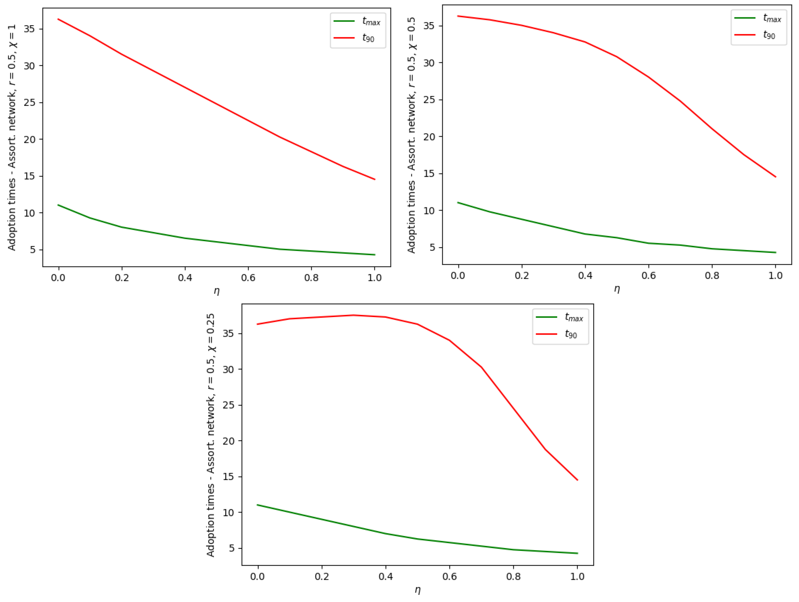
By implementing a cycle of repeated numerical solutions with increasing values of , we can check how the fraction of Enthusiasts (or correspondingly the fraction of Sceptics) influences the times and . Qualitatively, one expects that both times decrease with , and this is confirmed numerically (see Figure 6 and Figure 7). There is an anomaly, however, in the presence of strong polarization. As seen, for example, in the third graph of Figure 6, with a polarization , the time increases slightly at small , and then it reaches a maximum and decreases when . This happens because, with this value of polarization, an S-individual imitates an E-individual with a probability reduced by 75%. It follows that a population composed almost exclusively of Sceptics can paradoxically reach the 90% adoption level earlier than a population including approx. 1/3 of Enthusiasts.
5. Conclusions
Models of diffusion processes on networks consisting of coupled nonlinear equations in the mean-field approximation approach their technical limits when one also introduces, besides n connectivity classes, a considerable number K of behavioral classes.
In this work, after giving the general formulation of the equations, we thus focused our attention on the case and qualitatively analysed its phenomenology.
Already in the simplest case, when half the population consists of Enthusiasts and the other half of Sceptics and the network is uncorrelated, one notices a clear difference in the adoption curves of the two compartments: the peak of adoptions is reached earlier by E than by S, where for E the peak is higher, and after the peak the adoption rate decreases faster. Both these effects are considerably enhanced by the presence of strong polarization (when S individuals imitate, almost exclusively, other S individuals). The size of the network and the scale-free exponent appear to have little influence on the adoption curves. The effect of degree correlations is more pronounced: for assortative networks, the adoption peaks are approached more quickly in both the E and S compartments.
It should be stressed that the numerical integration of the equations is fast, thanks to the smooth character of the solutions, which allows the use of a second-order Euler algorithm (see Appendix A). We can thus expect that integration will also be reasonably fast with a larger number of behavioral compartments and with larger networks (for example, having a maximum node degree of or ). What becomes more difficult in the presence of many behavioral compartments is the interpretation of the results. For this purpose, machine learning methods could be employed in future work.
Clearly, even the introduction of many compartments does not allow to capture the entire complexity of a diffusion process, and agent-based simulations have also been employed in the literature (see, for example, Ref. [4]). Nevertheless, methods based on diffusion equations represent a useful benchmark for agent-based simulations as well.
As a further example of possible specialization of our differential equations, we considered the occurrence of strong opinion polarization in a population, such that individuals in a certain compartment almost exclusively imitate those from the same compartment. A different possibility, not considered in this work, is to define a model in which the degree distribution of the nodes of the underlying network is different in different compartments. In that case, Equations (12) and (13) are not valid and should be properly generalized.
Funding
This research received no external funding.
Institutional Review Board Statement
Not applicable.
Informed Consent Statement
Not applicable.
Data Availability Statement
Not applicable.
Conflicts of Interest
The authors declare no conflict of interest.
Appendix A. Python Code for Integration of the Equation System
#### INTEGRATION OF NETWORK BASS EQUATION WITH 2 COMPARTMENTS
from numpy import zeros
import matplotlib.pyplot as plt
eta=0.75
n=20 ## network max degree (corresp. to nr. of equations)
m=n+1
gamma=2.5 ## scale-free exponent
N=200 ## integration steps
dt=40/N ## 40: integration time interval
pE=0.03 ## publicity coefficient for enthusiasts
pS=0.01 ## publicity coefficient for sceptics
P=zeros(m,float)
## Definition of degree distribution
for k in range(1,m):
P[k]=1.0/k**gamma
## Normalization of degree distr.
norm=0
for k in range(1,m):
norm+=P[k]
P=P/norm
## calc. of <k>, used to renormalize the q coefficient
km=0
for k in range(1,m):
km+=k*P[k]
qE=0.35/km ## imitation coefficient for enthusiasts
qS=0.15/km ## imitation coefficient for sceptics
polariz=1 ## chi coefficient of polarization; chi=1 no polariz.
PP=zeros([m,m],float)
## definition of correlation matrix
for h in range(1,m):
for k in range(1,m):
PP[h,k]=h*P[h]/km ## uncorrelated matrix
## Definitions of various variable vectors
E=zeros([m],float) ## E relative population
S=zeros([m],float) ## S relative population
somma_E1=zeros([m],float) ## correlation sum for E in variation 1
somma_E2=zeros([m],float) ## correlation sum for E in variation 2
somma_S1=zeros([m],float) ## correlation sum for S in variation 1
somma_S2=zeros([m],float) ## correlation sum for S in variation 2
e1=zeros([m],float) ## variation 1 of E
e2=zeros([m],float) ## variation 2 of E
e=zeros([m],float) ## variation of E
s1=zeros([m],float) ## variation 1 of S
s2=zeros([m],float) ## variation 2 of S
s=zeros([m],float) ## variation of S
ee=zeros([m],float) ## derivative of E mult. by P
ss=zeros([m],float) ## derivative of S mult. by P
X=zeros([N+1],float)
Y=zeros([N+1],float)
Z=zeros([N+1],float)
## Start of integration cycle, with counter k
for k in range(0,N+1):
t=k*dt
## calculation of Euler variation 1 and 2 of the correlation terms
for i in range(1,m):
somma_E1[i]=0
somma_E2[i]=0
somma_S1[i]=0
somma_S2[i]=0
for i in range(1,m):
for j in range(1,m):
somma_E1[i]+=PP[j,i]*(eta*E[j]+(1-eta)*S[j])
somma_S1[i]+=PP[j,i]*(eta*polariz*E[j]+(1-eta)*S[j])
e1[i]=dt*(1-E[i])*(pE+qE*i*somma_E1[i])
s1[i]=dt*(1-S[i])*(pS+qS*i*somma_S1[i])
for i in range(1,m):
for j in range(1,m):
somma_E2[i]+=PP[j,i]*(eta*(E[j]+e1[j])+(1-eta)*(S[j]+s1[j]))
somma_S2[i]+=PP[j,i]*(eta*polariz*(E[j]+e1[j])+(1-eta)
*(S[j]+s1[j]))
e2[i]=dt*(1-(E[i]+e1[i]))*(pE+qE*i*somma_E2[i])
s2[i]=dt*(1-(S[i]+s1[i]))*(pS+qS*i*somma_S2[i])
## variations for the total population (sum over node degrees)
ee_tot=0
ss_tot=0
E_tot=0
S_tot=0
for i in range(1,m):
e[i]=(e1[i]+e2[i])/2
s[i]=(s1[i]+s2[i])/2
E[i]+=e[i]
S[i]+=s[i]
ee[i]=e[i]*P[i]*eta/dt
ss[i]=s[i]*P[i]*(1-eta)/dt
ee_tot+=ee[i]
ss_tot+=ss[i]
E_tot+=E[i]*P[i]*eta
S_tot+=S[i]*P[i]*(1-eta)
X[k]=k
Y[k]=ee_tot
Z[k]=ss_tot
line1, = plt.plot(X,Z)
line2, = plt.plot(X,Y)
plt.show()
References
- Bass, F.M. A new product growth for model consumer durables. Manag. Sci. 1969, 15, 215–227. [Google Scholar] [CrossRef]
- Meade, N.; Islam, T. Modelling and forecasting the diffusion of innovation–A 25-year review. Int. J. Forecast. 2006, 22, 519–545. [Google Scholar] [CrossRef]
- Gleeson, J.P. High-accuracy approximation of binary-state dynamics on networks. Phys. Rev. Lett. 2011, 107, 068701. [Google Scholar] [CrossRef] [Green Version]
- Kiesling, E.; Günther, M.; Stummer, C.; Wakolbinger, L.M. Agent-based simulation of innovation diffusion: A review. Cent. Eur. J. Oper. Res. 2012, 20, 183–230. [Google Scholar] [CrossRef]
- Fok, D.; Franses, P.H. Modeling the diffusion of scientific publications. J. Econom. 2007, 139, 376–390. [Google Scholar] [CrossRef] [Green Version]
- Goldenberg, J.; Han, S.; Lehmann, D.R.; Hong, J.W. The role of hubs in the adoption process. J. Mark. 2009, 73, 1–13. [Google Scholar] [CrossRef]
- Schilling, M.A.; Shankar, R. Strategic Management of Technological Innovation; McGraw-Hill Education: New York, NY, USA, 2019. [Google Scholar]
- Keeling, M.J.; Eames, K.T. Networks and epidemic models. J. R. Soc. Interface 2005, 2, 295–307. [Google Scholar] [CrossRef] [PubMed] [Green Version]
- Bertotti, M.L.; Brunner, J.; Modanese, G. The Bass diffusion model on networks with correlations and inhomogeneous advertising. Chaos Solitons Fractals 2016, 90, 55–63. [Google Scholar] [CrossRef] [Green Version]
- Bertotti, M.L.; Modanese, G. The Bass diffusion model on finite Barabasi–Albert networks. Complexity 2019, 2019, 6352657. [Google Scholar] [CrossRef]
- Bertotti, M.L.; Modanese, G. On the evaluation of the takeoff time and of the peak time for innovation diffusion on assortative networks. Math. Comput. Model. Dyn. Syst. 2019, 25, 482–498. [Google Scholar] [CrossRef]
- Vespignani, A. Modelling dynamical processes in complex socio-technical systems. Nat. Phys. 2012, 8, 32–39. [Google Scholar] [CrossRef]
- Li, S.; Jin, Z. Modeling and analysis of new products diffusion on heterogeneous networks. J. Appl. Math. 2014, 2014, 940623. [Google Scholar] [CrossRef] [Green Version]
- Manshadi, V.; Misra, S.; Rodilitz, S. Diffusion in random networks: Impact of degree distribution. In Proceedings of the 13th Workshop on Economics of Networks, Systems and Computation, Irvine, CA, USA, 18 June 2018; p. 1. [Google Scholar]
- Rogers, E. Diffusion of Innovations; Simon and Schuster: New York, NY, USA, 2010. [Google Scholar]
- Norton, J.A.; Bass, F.M. A diffusion theory model of adoption and substitution for successive generations of high-technology products. Manag. Sci. 1987, 33, 1069–1086. [Google Scholar] [CrossRef] [Green Version]
- Jiang, Z.; Jain, D.C. A generalized Norton–Bass model for multigeneration diffusion. Manag. Sci. 2012, 58, 1887–1897. [Google Scholar] [CrossRef] [Green Version]
- Krishnan, T.V.; Jain, D.C. Optimal dynamic advertising policy for new products. Manag. Sci. 2006, 52, 1957–1969. [Google Scholar] [CrossRef] [Green Version]
- Mahajan, V.; Muller, E.; Srivastava, R.K. Determination of adopter categories by using innovation diffusion models. J. Mark. Res. 1990, 27, 37–50. [Google Scholar] [CrossRef]
- Van den Bulte, C.; Joshi, Y.V. New product diffusion with influentials and imitators. Mark. Sci. 2007, 26, 400–421. [Google Scholar] [CrossRef] [Green Version]
- Øverby, H.; Audestad, J.A.; Szalkowski, G.A. Compartmental market models in the digital economy—Extension of the Bass model to complex economic systems. Telecommun. Policy 2023, 47, 102441. [Google Scholar] [CrossRef]
- Eryarsoy, E.; Delen, D.; Davazdahemami, B.; Topuz, K. A novel diffusion-based model for estimating cases, and fatalities in epidemics: The case of COVID-19. J. Bus. Res. 2021, 124, 163–178. [Google Scholar] [CrossRef] [PubMed]
- Fotouhi, B.; Rabbat, M.G. Degree correlation in scale-free graphs. Eur. Phys. J. B 2013, 86, 510. [Google Scholar] [CrossRef] [Green Version]
Figure 1.
Example of adoption curves for Enthusiasts and Sceptics when they each make up half of the population () and their publicity and imitation coefficients p and q are different, as displayed in the legend. The network is scale-free with exponent , maximum degree , and uncorrelated (). There is no strong polarization (; compare Figure 2).

Figure 2.
Same as in Figure 1, but with strong polarization (, meaning that the probability that a Sceptic imitates an Enthusiast is reduced by 80%). This clearly has the effect of further delaying adoption for Sceptics.
Figure 2.
Same as in Figure 1, but with strong polarization (, meaning that the probability that a Sceptic imitates an Enthusiast is reduced by 80%). This clearly has the effect of further delaying adoption for Sceptics.
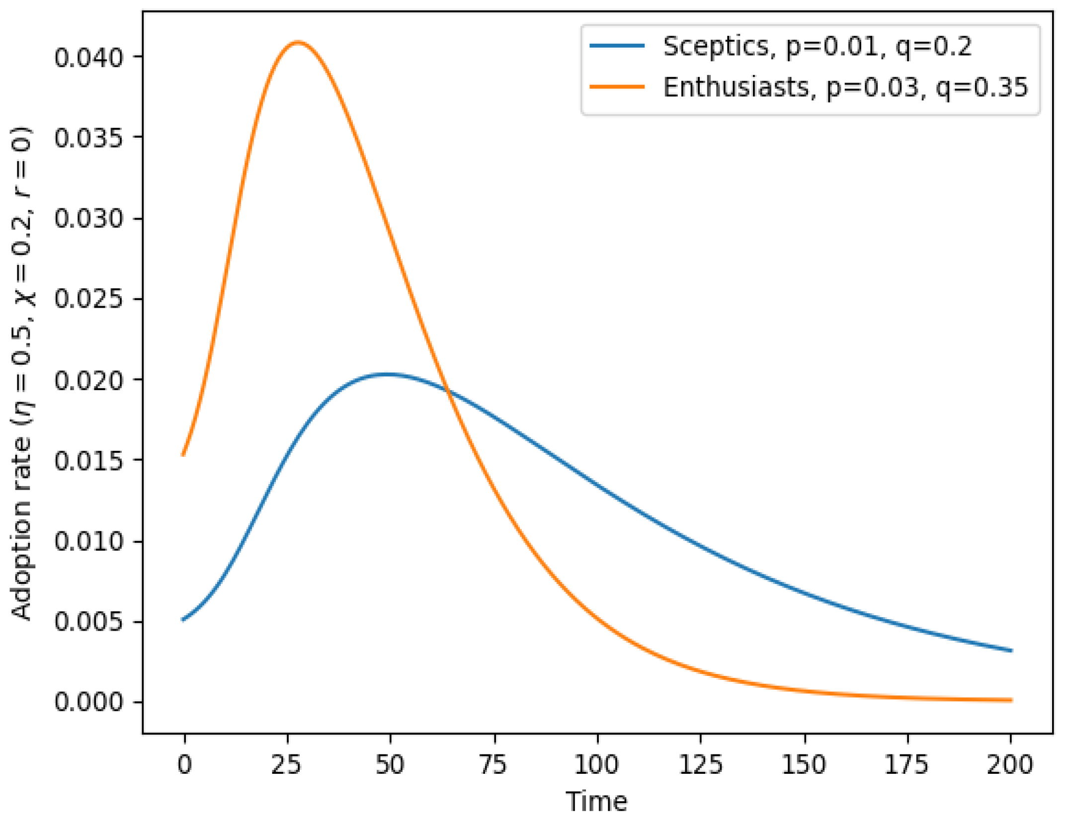
Figure 3.
Adoption rate as a function of time with a moderately assortative network having . (Left) No polarization (); (Right) strong polarization (). Compare Figure 1 and Figure 2 and see their captions for more details.

Figure 4.
Adoption rate as a function of time with a strongly assortative network having . (Left) No polarization (); (Right) strong polarization (). Compare Figure 1 and Figure 2 and see their captions for more details.
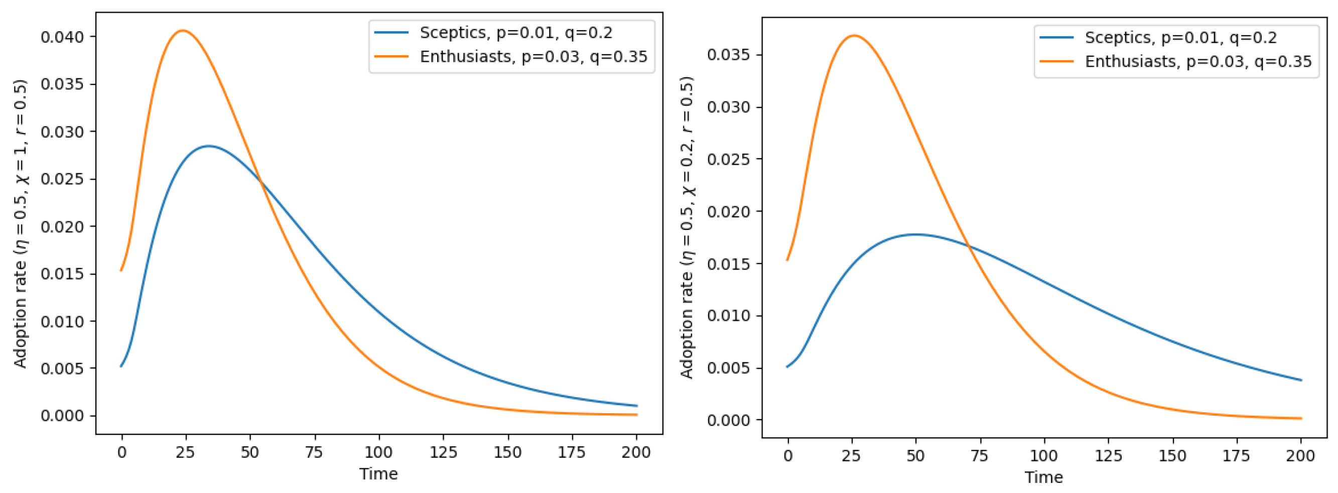
Figure 5.
Adoption rate as a function of time with a Barabasi–Albert network having (each new node is attached to one parent node in the growth of the network by preferential attachment). (Left) No polarization (); (Right) strong polarization (). Compare Figure 1 and Figure 2 and see their captions for more details.
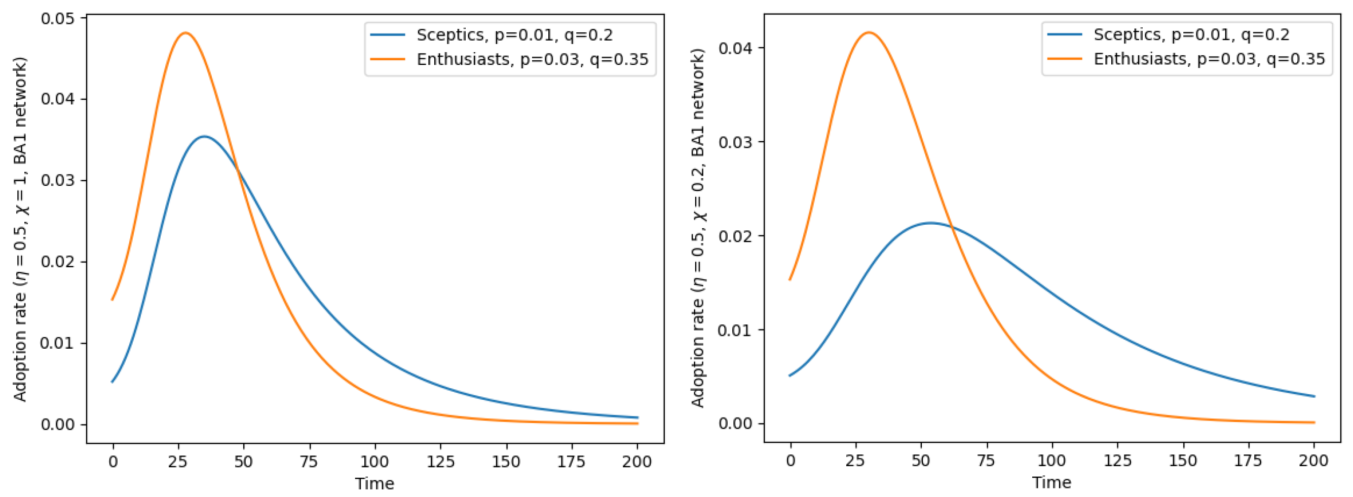
Figure 6.
Dependence of the adoption times and on the fraction of Enthusiasts in the population. Uncorrelated network, maximum degree , scale-free exponent ; increasing polarization in the three graphs.
Figure 6.
Dependence of the adoption times and on the fraction of Enthusiasts in the population. Uncorrelated network, maximum degree , scale-free exponent ; increasing polarization in the three graphs.
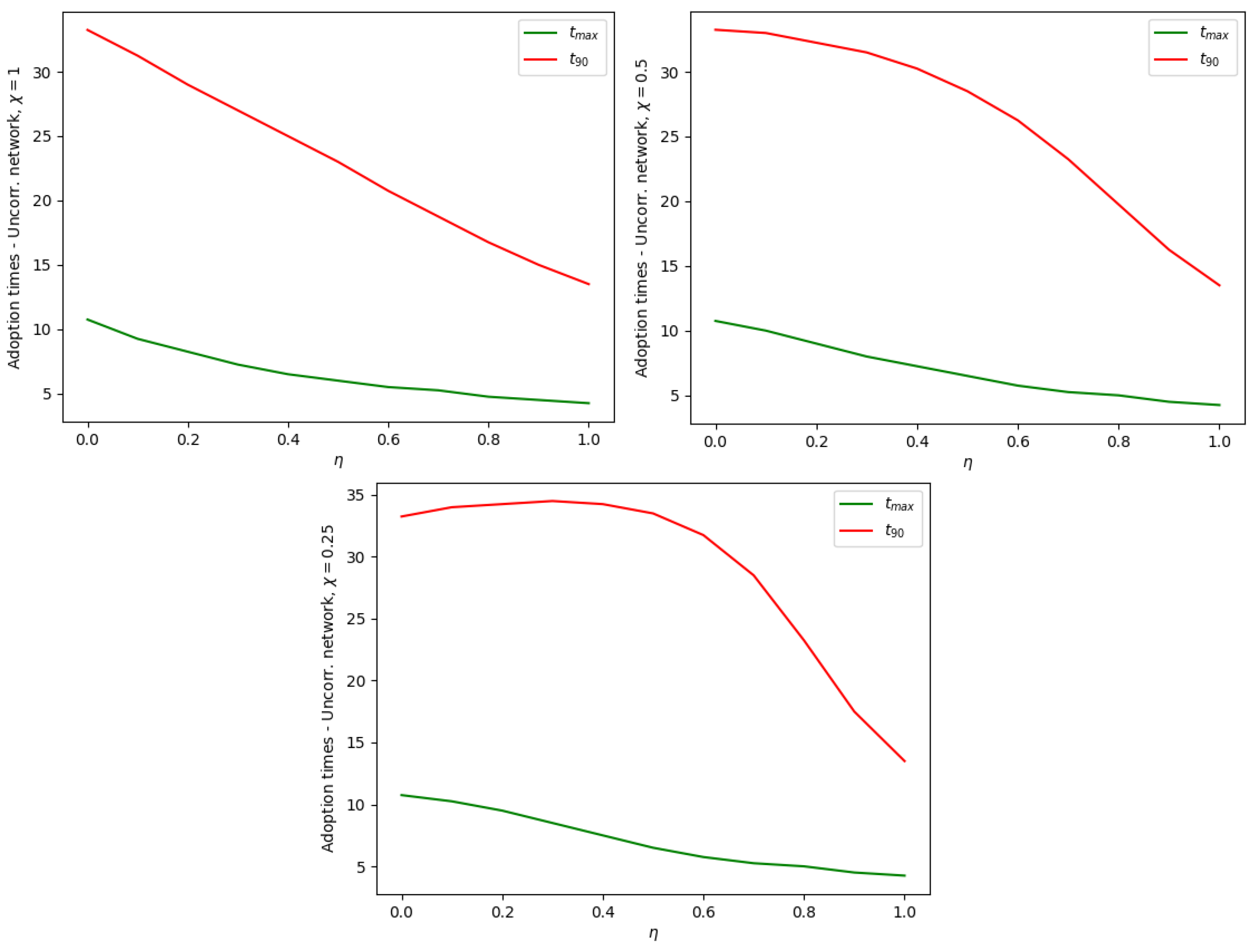
Figure 7.
Dependence of the adoption times and on the fraction of Enthusiasts in the population. Strongly assortative network (), maximum degree , scale-free exponent ; increasing polarization in the three graphs.
Figure 7.
Dependence of the adoption times and on the fraction of Enthusiasts in the population. Strongly assortative network (), maximum degree , scale-free exponent ; increasing polarization in the three graphs.
Disclaimer/Publisher’s Note: The statements, opinions and data contained in all publications are solely those of the individual author(s) and contributor(s) and not of MDPI and/or the editor(s). MDPI and/or the editor(s) disclaim responsibility for any injury to people or property resulting from any ideas, methods, instructions or products referred to in the content. |
© 2023 by the author. Licensee MDPI, Basel, Switzerland. This article is an open access article distributed under the terms and conditions of the Creative Commons Attribution (CC BY) license (https://creativecommons.org/licenses/by/4.0/).
Share and Cite
MDPI and ACS Style
Modanese, G. The Network Bass Model with Behavioral Compartments. Stats 2023, 6, 482-494. https://doi.org/10.3390/stats6020030
AMA Style
Modanese G. The Network Bass Model with Behavioral Compartments. Stats. 2023; 6(2):482-494. https://doi.org/10.3390/stats6020030
Chicago/Turabian StyleModanese, Giovanni. 2023. "The Network Bass Model with Behavioral Compartments" Stats 6, no. 2: 482-494. https://doi.org/10.3390/stats6020030