Abstract
Researchers conducting longitudinal data analysis in psychology and the behavioral sciences have several statistical methods to choose from, most of which either require specialized software to conduct or advanced knowledge of statistical methods to inform the selection of the correct model options (e.g., correlation structure). One simple alternative to conventional longitudinal data analysis methods is to calculate the area under the curve (AUC) from repeated measures and then use this new variable in one’s model. The present study assessed the relative efficacy of two AUC measures: the AUC with respect to the ground (AUC-g) and the AUC with respect to the increase (AUC-i) in comparison to latent growth curve modeling (LGCM), a popular repeated measures data analysis method. Using data from the ongoing Panel Study of Income Dynamics (PSID), we assessed the effects of four predictor variables on repeated measures of social anxiety, using both the AUC and LGCM. We used the full information maximum likelihood (FIML) method to account for missing data in LGCM and multiple imputation to account for missing data in the calculation of both AUC measures. Extracting parameter estimates from these models, we next conducted Monte Carlo simulations to assess the parameter bias and power (two estimates of performance) of both methods in the same models, with sample sizes ranging from 741 to 50. The results using both AUC measures in the initial models paralleled those of LGCM, particularly with respect to the LGCM baseline. With respect to the simulations, both AUC measures preformed as well or even better than LGCM in all sample sizes assessed. These results suggest that the AUC may be a viable alternative to LGCM, especially for researchers with less access to the specialized software necessary to conduct LGCM.
1. Introduction
Repeated measures designs are quite common in psychological research as they provide valuable information about the effects of time on psychological processes and behavior. Repeated measures designs, as the label implies, involve collecting data on the same individuals repeatedly over time. This has several important advantages over cross-sectional data analysis [1]. For instance, there is saving in recruiting costs and effort, as research requires fewer participants to achieve an acceptable power (e.g., ≥0.80) [2]. There is also an increase in power because of a reduction in measurement error through the elimination of individual differences (i.e., the same individual is measured over time). There are several data analysis strategies for dealing with repeated measures designs. Among these are repeated measures ANOVA, general estimating equations (GEE), multilevel modeling (i.e., mixed effects designs), and latent growth curve modeling (LGCM).
Repeated measures ANOVA is a very popular approach noted for its relative simplicity and its accessibility to individuals with moderate statistical knowledge and access to popular statistical computer packages (e.g., SPSS). However, it requires meeting assumptions such as sphericity (equality of variances of the differences among repeated measures: the univariate approach) and does not have an adequate method for dealing with missing data [3]. Furthermore, inappropriate use can lead to an inflation of the type I error rate (the familywise error rate), particularly when conducting post hoc analyses [1]. General estimating equations are an alternative with greater flexibility. Unlike repeated measures ANOVA, with GEE, researchers can select the best correlation structure among repeated measures (e.g., the autoregressive correlation structure: AR(1)), as well as specifying the appropriate link function [4,5]. Unfortunately, GEE assumes data are missing completely at random (MCAR), an often-untenable assumption, although there are some adjusted GEE methods for use when data are missing at random (MAR but not MCAR) [5,6]. Furthermore, there is no likelihood function in GEE, precluding model comparisons. Multilevel models permit for nesting, such as when data are nested within person (repeated measures) or when clustered within higher-level units such as family, classroom, or school. Multilevel models with repeated measures nested within the individual have good power so long as there is lower variability in the random effects and a larger sample size [7]. LGCM has similarities to these other methods [8,9,10]. Unlike multilevel modeling, however, LGCM does not segregate data into various levels, estimating parameters in a single model using latent variables to represent the initial level (baseline) and the rate of change over time (trend). Furthermore, unlike the other methods, LGCM generally employs full information maximum likelihood (FIML) parameter estimation, which allows for the use of all available data in estimating population parameters. As such, when using FIML, the sample sizes in LGCM are equal to the largest number of participants in any one of the modeled time points, minus any participants missing on covariates. In addition, since LGCM works within a structural equation modeling (SEM) framework, it affords tremendous flexibility in hypothesis testing, including the use of time invariant and time varying covariates, and assessing relations among parallel processes (e.g., two LGCMs with relations among the latent variables). Indeed, SEM can be used with other analysis methods (including multilevel modeling) if the correct software is employed (e.g., Mplus software) [11].
Unfortunately, with the exception of perhaps repeated measures ANOVA, these other methods either require specialized software or advanced understanding of research methods and data analysis to make the correct choices, such as the best fitting model when using LGCM. As such, a simpler method to analyze repeated measures data would benefit researchers interested in working with repeated measures data.
One method that is applied widely in various research endeavors but has only recently been applied with repeated measures designs in psychological and behavioral research is the area under the curve (AUC) [12]. Widely employed in the study of metabolic processes, such as daily cortisol, and receiver operating characteristic (ROC) curves, researchers have only recently applied the AUC to the assessment of behavior change (e.g., [13]). As such, the purpose of this study is to expand upon this research by assessing the relative efficacy of the AUC to one popular method, LGCM, by comparing the effects of select predictor variables on repeated measures of a dependent variable using the two methods. To accomplish this aim, we used secondary data from the Panel Study of Income Dynamics (PSID) Transition to Adulthood (TA) supplement (ages 18–28 years old), as this nationally representative dataset provides downloadable longitudinal data freely available for the assessment of researcher-initiated hypotheses. Our repeated measures dependent variable of choice was social anxiety (years 2005, 2007, 2009, and 2011). To assess the validity of our results, we identified four potential predictor variables that were available in the dataset and have been found to be related to social anxiety: biological sex, the tendency to worry, risk-taking behavior, and well-being [14,15,16,17,18,19]. After completing the initial assessments with both LGCM and the AUC, we used parameter estimates from these analyses as population parameters in Monte Carlo simulations. This allowed us to assess the parameter bias and power associated with the different sample sizes for the two methods.
2. Methods
2.1. Initial Analysis Using PSID Data
The participants were 741 18 to 28-year-old young adults (53% female) taking part in the PSID Transition to Adulthood (TA) supplement, years 2005–2011, with complete data on our four predictor variables: sex, worry, risk-taking behavior, and well-being. We chose these specific years to ensure the greatest sample size possible in the repeated measure variables. The PSID’s original 1968 sample included 18,000 individuals in 4800 families, including 1872 low-income families [20]. When descendants of the original families moved out and formed families of their own, they also became PSID families, and many agreed to take part in the ongoing study. The Child Development Supplement (CDS) was started in 1997 to follow up two randomly selected children (ages 0–12) born from PSID families and their caregivers (n = 3563). Adult children who left the original PSID households and established their own independent, economic households were invited to join the study via participation in the TA supplement, which collected data to better understand the social, health, and economic transitions of young adulthood [20].
2.2. Social Anxiety
For repeated measures of social anxiety, our variable is the average of four items (each rated 1–7) at each of the four time points: “How Often Nervous Meeting Others”, “How Often Feel Shy”, “How Often Feel Self-Conscious”, and “How Often Feel Nervous Performing”. The averages are based on complete data only.
2.3. Area under the Curve
We calculated the area under the curve (AUC) with two equations, one for AUC with respect to the ground (AUC-g) and one for AUC with respect to the increase (AUC-i) [21]. Area under the curve (AUC) is a common method to calculate probabilities in mathematical statistics via linear summation for discrete variables or integration for continuous variables [22]. To calculate each, these equations summate the areas of trapezoids between consecutive time points. Equation (1) presents the formula for calculating AUC-g in a situation with four time points, as we are employing four time points in this study. With four time points, there are three terms, one for the area of each trapezoid made by the consecutive measurements (height × width). Note that when calculating the AUC, one could simply summate adjacent rectangles. However, in doing so, only one corner of the rectangles touches the line representing change (trajectory) precisely, with the area between the line and the other top-side corner of the rectangle falling either below or above the line. Dividing by two compensates for this discrepancy, as is seen in Equation (1).
If we define the x-axis differences (intervals) as ti, where i represents the measurement time-point (ranging from 0 to n), there is one less interval than the number of time points. In the case of Equation (1), where there are four time points, there are n – 1 = 3 intervals. We can therefore reduce Equation (1) as follows:
If t is constant (i.e., an equal time interval across the repeated measures), Equation (2) becomes:
Pruessner and colleagues [21] noted that one possibility when the intervals are constant is to define the interval as 1, thereby eliminating ti from the equation altogether, precluding, however, the ability to label the equation as an area under the curve.
Equation (4) presents the formula for AUC-i. It includes the same terms as Equation (1) through Equation (3), with the addition of a subtraction term to account for the change from the baseline. This term, however, makes it possible for a negative value, removing the ability to define Equation (4) as an area.
More generally, and substituting ti for interval, this equation reduces to:
If the intervals are equal (constant), Equation (5) reduces to:
2.4. Predictor Variables
The predictor variables we used in this study are biological sex (1 = male; 0 = female), well-being, worry, and risk-taking behavior. Well-being is an average of three subscales (non-missing data only): emotional well-being, social well-being, and psychological well-being. Emotional well-being was the average of three items (each rated 1–6): “Frequency of Happiness in the Last Month”, “Frequency of Interest in life in the Last Month”, and “Frequency of Feeling Satisfied in the Last Month”. Social well-being is the average of five items (each rated 1–6): “Frequency of Feeling Something to Contribute to Society”, “Frequency of Feeling Belonging to a Community”, “Frequency of Feeling Society Getting Better”, “Frequency of Feeling People Basically Good”, and “Frequency of Feeling Way Society Works Makes Sense”. Psychological well-being was the average of six items (each rated 1–6): “Frequency of Feeling Good at Managing Daily Responsibility”, “Frequency of Feeling Has Trusting Relationships with Others”, “Frequency of Feeling Challenged to Grow”, “Frequency of Feeling Confident of Own Ideas”, “Frequency of Feeling Liked Own Personality”, and “Frequency of Feeling Life Had Direction”. Worry was the average of three items (each rated 1–7; non-missing data only): “How Often Worry About Money”, “How Often Worry About Future Job”, and “How Often Feel Discouraged About Future”. Risk was the average of five items (each rated 1–7; non-missing data only): “How Often Did Something Dangerous”, “How Often Damaged Public Property”, “How Often Got into Physical Fight”, “How Often Drove When Drunk or High”, and “How Often Rode with Drunk Driver”.
2.5. Data Analysis and Statistics
We conducted data analysis using latent growth curve modeling (LGCM) and multiple regression analysis. We also conducted Monte Carlo simulations to compare the performance of the two AUC regression equations and LGCM under different sample sizes, including the estimation of bias and power. In all models assessed, repeated measures of social anxiety were the dependent variables, whether as part of the LGCM or elements of the AUC equations. We used Mplus version 8.3 for all modeling [23]. We used SPSS version 28 for descriptive statistics.
2.5.1. Latent Growth Curve Modeling
Latent growth curve modeling is a structural equation modeling (SEM) method that involves estimating individual developmental trajectories from repeated measures of observed variables [8,10]. LGCM uses latent (unobserved) variables to model the initial level (baseline) and the rate of change from the baseline (e.g., linear or quadratic trends). A basic growth model includes one latent variable for the baseline (intercept) and one for a linear trend. Using matrix symbols [24,25,26], the t repeated observed measures are regressed on the set of latent variables representing the initial level and the rate of change, along with the residual variance not accounted for by the model (measurement model; Equation (7)). Note that y is a vector of the t repeated measures (t—dimensional vector). Λ is a t x m matrix relating the m latent variables (eta; η vector) to the t repeated measures. ε (epsilon) is a t-dimensional vector of residuals. Equation (8) is the structural part of the model (structural model), in which one can regress latent variables on other latent or measured variables. α (alpha) is a vector containing intercept parameters relating the predictor variables to the latent variables. B (beta) is an m × m matrix of parameters from regressing latent variables on other latent variables, such as when we have two parallel LGCMs and are interested in how change in one process affects change in the other process. Gamma (Γ) is an m × p matrix of regression coefficients relating the p predictor variables (covariates; x) to the latent variables. Sigma (ς) is an m-dimensional vector of residuals.
Expand on Equation (7), with t = 4 time points and a linear trend factor and use matrix algebra (a matrix is defined by its size (rows × columns)). Addition is cell to cell between equally sized matrices (i.e., matrices of the same dimension). For multiplication, the inner terms must be equal. For instance, we can multiply a 2 × 2 matrix by a 2 × 3 matrix since the columns for the first matrix equal the rows for the second matrix (i.e., the two inner terms). The product is a matrix whose dimension is the two outer terms. In this example, it is a 2 × 3 matrix.), and we obtain:
Note that the yi represent each individual’s outcome score for a given repeated measure, and π0i and π1i are the latent variables, intercept and trend, respectively, representing individual i’s trajectory.
Expanding upon Equation (8), with four measured predictor variables (as in the present analysis) and no latent predictor variables (i.e., excluding the second term to the right of the equal sign in Equation (8)), we obtain:
Thus, as an example, for the intercept, our model would be:
Graphically, we can represent the LGCM using ovals for latent variables and rectangles for the repeated observed measures (Figure 1). Notice that the coefficients emanating from each factor to the measured variable (factor loadings) are fixed values, with the loadings from the baseline level constrained to equal one, meaning that the relationship between the baseline level and the measured variables remains constant across repetitions. Furthermore, the relationship between each measured variable and the linear trend latent variable increase in a linear fashion from the baseline. This can be relaxed, though, allowing the effect of time to be freely estimated [24]. Finally, the curved arrow connecting the two latent variables represents a correlation.
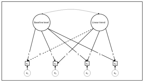
Figure 1.
Basic latent growth curve measurement model.
For our LGCM models, we will judge the model fit using the following criteria: the Pearson chi-square goodness of fit test, the comparative fit index (CFI), the root mean square error of approximation (RMSEA), and the standardized root mean residual (SRMR). The suggested criteria for good fit using these criteria are a non-significant chi-square, an CFI ≥ 0.95, an RMSE ≤ 0.06, and an SRMR ≤ 0.05 [27].
2.5.2. Multiple Imputation
We conducted multiple imputation with our four repeated measures of social anxiety to account for missing data in the calculation of our two AUC variables. Multiple imputation involves randomly generating a selected number (n) of replacement values (imputations) for missing data points, running the model for each imputed dataset, and then averaging parameter estimates across the n imputations [28]. We used Mplus to conduct the multiple imputations with n = 50 imputations [23,29].
2.5.3. Monte Carlo Simulations
The simulations in this study employed parameter estimates saved from the LGCM and multiple regression analyses. Mplus permits for saving estimates from analyses for use in Monte Carlo simulations. These estimates were subsequently employed as population parameters for the subsequent simulations with six different sample sizes (LGCM: 741, 500, 250, 100, and 50). For the AUC Monte Carlo models, we did not employ the exact same process for our parameter estimates, as Mplus does not save estimates from the averaged multiple imputation parameters. As such, we took the estimates from the averaged imputation model and manually generated our dataset of parameter estimates for all subsequent AUC Monte Carlo models. With this model as our population model, we ran simulations with n = 555 (the sample size from the original AUC calculations deleting cases list-wise), 741, 500, 250, 100, and 50. To assess the performance of each simulated model with the different sample sizes, we used the average estimate of the population parameters, % Bias (comparing the average estimate to the population parameter), mean square error (MSE), coverage (where 95% of all values should fall within the 95% confidence interval), and power [23]. The Mplus code for the Monte Carlo analyses along with the data files with parameter estimates are included as supplementary files.
3. Results
3.1. Descriptive Statistics
Table 1 presents the frequencies and percentages for our discrete model variables and the means and standard deviations for all continuous model variables. We include skewness and kurtosis statistics for our two AUC measures, along with the four social anxiety repeated measures used to generate the AUC measures. Assessing the Kolmogorov–Smirnov and Shapiro–Wilk’s tests, both AUC-g and AUC-i and the four social anxiety repeated measures, diverged from normality, p < 0.05; although, these statistics are somewhat less reliable when the sample size is large [30,31]. Visual inspection of the histograms in Figure 2 (panels A through D) suggests relative minor divergence from normality, for social anxiety 2009 through 2011, respectively. Likewise, for AUC-g and AUC-i (Figure 3, panels A and B, respectively 3) the divergence from normality was not major. This is supported by the ratios of the estimates to the standard errors for our two AUC measures, with the maximum ratio being 2.7 (AUC-g skewness). This too is supported by the ratios of the estimates to the standard errors among the four SA measures; although, the kurtosis to standard error ratios were higher for SA 2005 and 2007, with them being 4.346 and 3.272, respectively. Although standard errors for the skewness and Kurtosis statistics can be problematic if the variables are not normally distributed [32], the estimate to standard error ratios in Table 1 tend to support the likelihood that our AUC measures are normal or close to normal in distribution.

Table 1.
Descriptive statistics.
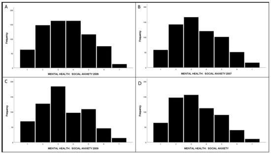
Figure 2.
Histograms for the four social anxiety repeated measures (panels (A)–(D)).
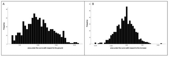
Figure 3.
Histograms for the AUC-g (panel (A)) and AUC-i (panel (B)).
3.2. Latent Growth Curve Model
We began by fitting a crude LGCM to the data (measurement model). The crude model excludes all predictor variables and allows us to assess the best fitting model to the data (e.g., linear or quadratic). A model with a linear trend fitted the data well: Χdf=5, n=2155 = 4.019, p = 0.547, CFI = 1.00, and RMSEA = 0.00 (90% CI: 0.00–0.027). There was an overall significant decline in social anxiety from baseline (B = −0.066, z = −4.311, p < 0.0001). We next added the four covariates to the model: sex, risk, well-being, and worry. Regressing the baseline/intercept and trend factors on the four covariates, this model also fitted the data well: Χdf=13, n=741 = 10.760, p = 0.6309, CFI = 1.00, and RMSEA = 0.00 (90% CI: 0.00–0.031), SRMR = 0.017. We present the results of the LGCM regression in Table 2. All covariates except sex had significant effects on baseline social anxiety. Well-being (p < 0.0001) and risk (p = 0.003) were negatively associated with social anxiety at baseline, whereas worry (p < 0.0001) was positively associated with baseline social anxiety. For the linear trend from baseline (slope), risk was positively (p = 0.026) and worry (p = 0.048) negatively related to the rate of change.
Table 2.
Multivariate modeling results for LGCM and AUC.
3.3. AUC-g
For the area under the curve with respect to the ground, we ran a multiple regression analysis to assess the effects of each of the four covariates on the AUC-g measure. Given AUC-g that is a simple linear summation of polygons (Equations (1)–(3)), any participant with missing data at a given time point was automatically eliminated from the calculation. As such, the final sample size for our regression analysis was n = 555, after accounting for missing data on the covariates. This compares to n = 741 for the LGCM, which relies on FIML for parameter estimation in Mplus. For AUC-g, well-being and worry had significant effects on AUC-g, with well-being negatively (p < 0.0001) and worry positively (p < 0.0001) related to social anxiety (Table 2).
3.4. AUC-i
For the area under the curve with respect to the increase (Table 2), there were no significant effects on AUC-i.
3.5. Multiple Imputation Analysis for the Area under the Curve
We reran the regression analyses for both AUC measures with the multiple imputation data. We present the results with the averaged imputed parameter estimates in Table 2. The effects of sex (p = 0.023), risk (p = 0.032), well-being (p < 0.0001), and worry (p < 0.0001) on AUC-g were significant and resembled the results (in direction) seen for these predictors on baseline LGCM. However, whereas the effect of sex on AUC-g was significant, it was not significant for the LGCM either at baseline or with the linear trend. Like the non-imputed results, there were no significant effects of any covariate AUC-i.
3.6. Monte Carlo Simulation Studies
3.6.1. LGCM
We present the results from our simulation studies with LGCM in Table 3. Bias and power for the effects of the predictor variables on the baseline level were good at n = 741, with the exception of the effect of sex (power = 0.274). The opposite was the case for the effect of the predictor variables on the linear trend. Not one effect had a power greater than 0.641 (risk). The lowest power was with sex (power = 0.102), meaning there was only a 10% chance of rejecting a false null hypothesis, even with 741 participants. As the sample sizes decreased to n = 50, the power decreased particularly with the effects on the linear trend. Similarly, bias increased as the sample size decreased, particularly for the effects on the trend factor and at the smaller sample sizes, reaching as high as −11.7 for the effect of sex on the linear trend with n = 100.
Table 3.
Simulation results for the LGCM.
3.6.2. AUC
We present the results for multiple regression simulation studies assessing the effects of the predictor variables on the two AUC variables in Table 4. Bias was lower in all but a few cases for both AUC-g and AUC-i when compared to LGCM, with bias reaching 6.27% for the effect of well-being on AUC-i when n = 250. Power was generally higher than for LGCM, although primarily for AUC-g, and especially at the larger sample sizes. At n = 50, the power was generally the same and even better for the effects of all variables on the LGCM baseline level when compared to the two AUC variables. A direct comparison of % bias and power values are made in Table 5, with the highest absolute % bias and power values in bold for each specific effect.
Table 4.
Simulation results for the AUC models.
Table 5.
Comparison of % bias and power values.
4. Discussion
The present study aimed to extend prior work looking at the performance of the AUC as a dependent variable representing repeated measures of a variable of interest [12]. The results support AUC as a viable alternative to LGCM when assessing the effects of predictor variables on repeated measures of a continuous variable. Using AUC-g and AUC-i as dependent variables in regression analysis, these summary variables performed as well as LGCM, with a particular advantage over models including effects of predictor variables on the rate of change from baseline. The difference was especially pronounced when the predictor variable was binary, such as biological sex. Although power was not impressive in either model (LGCM or the AUC), it was superior in the AUC analysis, particularly with respect to the ground. Nevertheless, LGCM has some important advantages over the AUC when assessing effects on repeated measures of a certain variable. For instance, LGCM permits the partitioning of trajectories into an intercept and a trend, allowing a researcher to ascertain effects of predictor variables beyond that seen at a cross-section (baseline). However, this advantage comes with complexity, particularly when the best fitting model includes higher-order powers, such as a quadratic or cubic trend. Interpreting such effects is complicated and perhaps unnecessary. The simplicity of the AUC in contrast is the use of a single variable to represent both the initial level and change, with one mean and one standard deviation. Given that both AUC measures are calculated by summing adjacent trapezoids, it easily captures fluctuations in the variable being modeled across time. Furthermore, for researchers desiring to better understand what effects are happening post baseline using the AUC, one can either rely on AUC-i or disaggregate the data into individual trajectories for further analysis.
Despite these benefits, there are some hurdles to the use of the AUC universally in repeated measures designs. For instance, the possibility of negative values for AUC-i is problematic, as the area cannot be negative. Identifying alternative equations would benefit researchers preferring to avoid negative area calculations. Another problem may be the use of AUC with large numbers of repeated measures. For instance, in ecological momentary assessment studies, there are large numbers of repeated measures, making calculations using the present equations time intensive to code. Alternative methods that estimate curves instead of summating polygons as we performed here, such as perhaps using a Taylor series approximation before integration to the calculate area, may be better options in such cases. These limitations notwithstanding, the AUC is a viable method that researchers can add to their research quivers. Future studies should expand upon this and other studies by examining the AUC’s performance as a predictor variable and comparing the AUC to other repeated measures methods such as GEE and mixed effects models.
Supplementary Materials
The following supporting information can be downloaded at: https://www.mdpi.com/article/10.3390/stats6020043/s1, We included the Mplus syntax for the Monte Carlo simulations, as well as the data files including the parameter estimates used as input for the simulations, as supplementary files.
Funding
This study did not receive any funding.
Institutional Review Board Statement
IRB approval was not required for this study.
Informed Consent Statement
Not applicable.
Data Availability Statement
Data are available upon request.
Conflicts of Interest
There are no conflicts of interest to report.
References
- Pituch, K.A.; Stevens, J.P. Applied Multivariate Statistics for the Social Sciences: Analyses with SAS and IBM’s SPSS; Routledge: London, UK, 2015. [Google Scholar]
- Rodriguez, D. Research Methods; Kendall Hunt Publishing Company: Dubuque, IA, USA, 2021. [Google Scholar]
- Park, E.; Cho, M.; Ki, C.-S. Correct use of repeated measures analysis of variance. Korean J. Lab. Med. 2009, 29, 1–9. [Google Scholar] [CrossRef] [PubMed]
- Liang, K.-Y.; Zeger, S.L. Longitudinal data analysis using generalized linear models. Biometrika 1986, 73, 13–22. [Google Scholar] [CrossRef]
- Robins, J.M.; Rotnitzky, A.; Zhao, L.P. Analysis of semiparametric regression models for repeated outcomes in the presence of missing data. J. Am. Stat. Assoc. 1995, 90, 106–121. [Google Scholar] [CrossRef]
- Yang, C.; Diao, L.; Cook, R.J. Adaptive response—Dependent two—Phase designs: Some results on robustness and efficiency. Stat. Med. 2022, 41, 4403–4425. [Google Scholar] [CrossRef] [PubMed]
- Lane, S.P.; Hennes, E.P. Power struggles: Estimating sample size for multilevel relationships research. J. Soc. Pers. Relatsh. 2018, 35, 7–31. [Google Scholar] [CrossRef]
- Duncan, T.E.; Duncan, S.C. An introduction to latent growth curve modeling. Behav. Ther. 2004, 35, 333–363. [Google Scholar] [CrossRef]
- Muthén, B.O.; Curran, P.J. General longitudinal modeling of individual differences in experimental designs: A latent variable framework for analysis and power estimation. Psychol. Methods 1997, 2, 371. [Google Scholar] [CrossRef]
- Duncan, T.E.; Duncan, S.C. The ABC’s of LGM: An introductory guide to latent variable growth curve modeling. Soc. Personal. Psychol. Compass 2009, 3, 979–991. [Google Scholar] [CrossRef] [PubMed]
- Schminkey, D.L.; von Oertzen, T.; Bullock, L. Handling missing data with multilevel structural equation modeling and full information maximum likelihood techniques. Res. Nurs. Health 2016, 39, 286–297. [Google Scholar] [CrossRef]
- Rodriguez, D. Assessing Area under the Curve as an Alternative to Latent Growth Curve Modeling for Repeated Measures Zero-Inflated Poisson Data: A Simulation Study. Stats 2023, 6, 22. [Google Scholar] [CrossRef]
- Campbell, R.L.; Cloutier, R.; Bynion, T.M.; Nguyen, A.; Blumenthal, H.; Feldner, M.T.; Leen-Feldner, E.W. Greater adolescent tiredness is related to more emotional arousal during a hyperventilation task: An area under the curve approach. J. Adolesc. 2021, 90, 45–52. [Google Scholar] [CrossRef]
- Hearn, C.S.; Donovan, C.L.; Spence, S.H.; March, S. A worrying trend in Social Anxiety: To what degree are worry and its cognitive factors associated with youth Social Anxiety Disorder? J. Affect. Disord. 2017, 208, 33–40. [Google Scholar] [CrossRef]
- Mick, M.A.; Telch, M.J. Social Anxiety and History of Behavioral Inhibition in Young Adults. J. Anxiety Disord. 1998, 12, 1–20. [Google Scholar] [CrossRef] [PubMed]
- Morrison, A.S.; Heimberg, R.G. Social anxiety and social anxiety disorder. Annu. Rev. Clin. Psychol. 2013, 9, 249–274. [Google Scholar] [CrossRef]
- Asher, M.; Asnaani, A.; Aderka, I.M. Gender differences in social anxiety disorder: A review. Clin. Psychol. Rev. 2017, 56, 1–12. [Google Scholar] [CrossRef] [PubMed]
- Doré, I.; O’Loughlin, J.; Sylvestre, M.-P.; Sabiston, C.M.; Beauchamp, G.; Martineau, M.; Fournier, L. Not flourishing mental health is associated with higher risks of anxiety and depressive symptoms in college students. Can. J. Community Ment. Health 2020, 39, 33–48. [Google Scholar] [CrossRef]
- Kashdan, T.B.; Collins, R.L.; Elhai, J.D. Social anxiety and positive outcome expectancies on risk-taking behaviors. Cogn. Ther. Res. 2006, 30, 749–761. [Google Scholar] [CrossRef]
- Panel Study of Income Dynamics; Public Use Dataset; University of Michigan: Ann Arbor, MI, USA, 2012.
- Pruessner, J.C.; Kirschbaum, C.; Meinlschmid, G.; Hellhammer, D.H. Two formulas for computation of the area under the curve represent measures of total hormone concentration versus time-dependent change. Psychoneuroendocrinology 2003, 28, 916–931. [Google Scholar] [CrossRef]
- Hogg, R.; McKean, J.; Craig, A. Introduction to Mathematical Statistics, 6th ed.; Pearson Prentice Hall: Upper Saddle River, NJ, USA, 2004. [Google Scholar]
- Muthén, L.K.; Muthén, B.O. Mplus User’s Guide, 8th ed.; Muthén & Muthén: Los Angeles, CA, USA, 1998. [Google Scholar]
- Muthén, B.O. beyond SEM: General latent variable modeling. Behaviormetrika 2002, 29, 81–117. [Google Scholar] [CrossRef]
- Willett, J.B.; Bub, K.L. Latent growth curve analysis. In Encyclopedia of Statistics in the Behavioral Sciences; John Wiley and Sons: Sussex, UK, 2004. [Google Scholar]
- Hancock, G.R.; Choi, J. A vernacular for linear latent growth models. Struct. Equ. Model. 2006, 13, 352–377. [Google Scholar] [CrossRef]
- Hooper, D.; Coughlan, J.; Mullen, M. Evaluating model fit: A synthesis of the structural equation modelling literature. In Proceedings of the 7th European Conference on Research Methodology for Business and Management Studies, London, UK, 19–20 June 2008; pp. 195–200. [Google Scholar]
- Little, R.J.A.; Rubin, D.B. Statistical Analysis with Missing Data, 2nd ed.; John Wiley & Sons, Inc: Hoboken, NJ, USA, 2002. [Google Scholar]
- Asparouhov, T.; Muthén, B. Multiple imputation with Mplus. MPlus Web Notes 2010, 29, 238–246. [Google Scholar]
- Matore, E.M.; Khairani, A.Z. The pattern of skewness and kurtosis using mean score and logit in measuring adversity quotient (AQ) for normality testing. Int. J. Future Gener. Commun. Netw. 2020, 13, 688–702. [Google Scholar]
- Demir, S. Comparison of normality tests in terms of sample sizes under different skewness and Kurtosis coefficients. Int. J. Assess. Tools Educ. 2022, 9, 397–409. [Google Scholar] [CrossRef]
- Wright, D.B.; Herrington, J.A. Problematic standard errors and confidence intervals for skewness and kurtosis. Behav. Res. Methods 2011, 43, 8–17. [Google Scholar] [CrossRef] [PubMed]


Disclaimer/Publisher’s Note: The statements, opinions and data contained in all publications are solely those of the individual author(s) and contributor(s) and not of MDPI and/or the editor(s). MDPI and/or the editor(s) disclaim responsibility for any injury to people or property resulting from any ideas, methods, instructions or products referred to in the content. |
© 2023 by the author. Licensee MDPI, Basel, Switzerland. This article is an open access article distributed under the terms and conditions of the Creative Commons Attribution (CC BY) license (https://creativecommons.org/licenses/by/4.0/).