Abstract
Factor analysis, a staple of correlational psychology, faces challenges with ordinal variables like Likert scales. The validity of traditional methods, particularly maximum likelihood (ML), is debated. Newer approaches, like using polychoric correlation matrices with weighted least squares estimators (WLS), offer solutions. This paper compares maximum likelihood estimation (MLE) with WLS for ordinal variables. While WLS on polychoric correlations generally outperforms MLE on Pearson correlations, especially with nonbell-shaped distributions, it may yield artefactual estimates with severely skewed data. MLE tends to underestimate true loadings, while WLS may overestimate them. Simulations and case studies highlight the importance of item psychometric distributions. Despite advancements, MLE remains robust, underscoring the complexity of analyzing ordinal data in factor analysis. There is no one-size-fits-all approach, emphasizing the need for distributional analyses and careful consideration of data characteristics.
1. Introduction
In 1904, Charles Spearman introduced a groundbreaking statistical methodology aimed at uncovering latent variables—those not directly measurable but estimable through observed correlations. Spearman’s approach, inspired by the pioneering work of Galton and Pearson, sought to operationalize the existence of two intelligence factors inferred from children’s school performance. He posited a general intelligence factor (G factor) and a specific intelligence factor (S factor), suggesting that positive correlations across seemingly unrelated subjects indicated these underlying factors [1]. Spearman’s formulation of factor analysis provided a framework that would become essential in the field of psychometrics, facilitating the identification and measurement of intangible psychological constructs.
Although Spearman’s theory of intelligence factors faced challenges from researchers like Thomson [2] and Thurstone [3], his method, exploratory factor analysis (EFA), became a cornerstone in psychometrics. This approach enabled researchers to estimate latent attributes such as intelligence, personality traits, and other psychological characteristics, contributing significantly to the development of psychological assessment. The foundational principles of EFA have endured, with modern adaptations expanding its utility across various domains of psychological and social science research.
Around the same period, Rensis Likert [4] introduced his influential scale to measure opinions and attitudes. This scale, originally composed of seven-point response items coded from 1 to 7, quickly gained popularity in psychology and remains widely used today for assessing latent psychometric variables. Likert scales are particularly valued for their simplicity and ease of use, making them a staple in both academic research and applied settings.
The main objective of this paper is to critically examine the challenges and controversies surrounding the application of factor analysis to ordinal data, such as that derived from Likert-type scales. Despite the widespread use of Likert scales and similar ordinal measures in psychological assessments, the validity of applying traditional factor analysis techniques to these types of data remains contentious. The paper seeks to explore both historical and contemporary perspectives on this issue, evaluating the adequacy of various methodological approaches and proposing potential solutions to improve the accuracy and reliability of factor analysis when applied to ordinal data.
Recent research has highlighted the complexities inherent in factor analyzing ordinal data, with scholars like Muthén and Kaplan [5] advocating for the use of robust statistical techniques that account for the noncontinuous nature of ordinal variables. More recent discussions by researchers such as Li [6,7] and Rhemtulla, Brosseau-Liard, and Savalei [8] emphasize the importance of choosing appropriate estimation methods, such as polychoric correlations and robust maximum likelihood estimation, to mitigate the biases that can arise when traditional methods are applied to ordinal data. Moreover, Liddell and Kruschke [9] and Foldnes and Grønneberg [10] underscore the ongoing debates and the need for careful consideration of both traditional and modern solutions to address these challenges.
Factor analysis continues to play a crucial role in uncovering the latent constructs assessed by Likert and similar rating scales, but the debate over the best practices for analyzing ordinal items remains unresolved. This paper aims to contribute to this discourse by providing a comprehensive review of the current state of the field, identifying gaps in the literature, and offering practical recommendations for researchers dealing with ordinal data in factor analysis.
1.1. Factor Analysis
Factor analysis aims to uncover latent variables through observed correlations. For instance, in the Beck Depression Inventory (BDI), responses to mood-related items reflect latent depression, with correlations among these items indicating its presence. Spearman’s factor analytic model explains observed variables’ behavior through latent factors. Thurstone [3] and Cattell [11] expanded this model, introducing exploratory factor analysis (EFA) with a reduced set of common factors and specific factors for each variable. Here a set of observed variables (X1, X2,… Xp) can be explained by a reduced m common factors (m << p) and p specific factors as (For an extensive account of the development of factor analysis see, e.g., Bartholomew [12]:
where μi represents the expected value of variable xi, λik represents the loading of factor k (k ∈ {1, …, m}) on variable i, fkj represents the common factor k for individual j (j ∈ {1, …, n}), and εij represents the residual or specific factor associated with observed variable Xi (i ∈ {1, …, p}) on individual j. Common factors are assumed to be independent, and specific factors are assumed to be independent and normally distributed.
The factor analysis can be carried out on the covariance matrix of the observed variables estimated as:
whose generic element is Galton’s covariance:
Since variables in the social sciences and humanities often have different scales and ranges of measurement, it is common to standardize them, centering the mean to 0 and reducing the standard deviation to 1 as . The variance–covariance matrix is then reduced to the matrix of the product–moment correlations, also known as Pearson’s correlations:
whose generic element is Pearson’s well-known correlation coefficient:
Using standardized variables, model (1.1) can now be written in matrix form as:
where Λ is a matrix of factor loadings, f is a vector of common factors, and ε is a vector of specific factors. From model 6, the correlation matrix can then be written as:
where ψ is the diagonal covariance matrix of the specific factors. Common factor loadings can be estimated from Equation (7). However, this equation is nonidentified (The system has p(p + 1)/2 known quantities and (m + 1)p (matrix mp and p vector quantities with m<< p)), so Spearman, in his “method of correlations” followed Pearson’s Principal Components method for factorizing the correlation matrix. The variables’ communality (see Equation (2)) is, therefore, estimated as the eigenvalues of the principal components retained from the correlation matrix. More recent methods of extraction of the common factors include the principal axis factoring method and the maximum likelihood method [13]. In short, the principal axis factorization method considers that the initial communalities are the coefficient of determination of each variable regressed on all others (and not 1, as in the principal components method), proceeding with an analysis of principal components in an optimization algorithm that stops when the extracted communalities reach their maxima. The maximum likelihood method, as proposed by Lawley and Maxwell [14], estimates the factor loadings that maximize the likelihood of sampling the matrix of observed correlations in the population. The solution is obtained by minimizing the maximum likelihood (ML) function (For a more detailed description, see e.g., [15]).
for Λ and ψ by a two-step algorithm that estimates the eigenvalues (common factor variance) and specific factor variances of the correlation matrix R calculated from the p observed variables.
Since the late 1960’s, the maximum likelihood method has been widely used in confirmatory factor analysis (CFA) [15]. In CFA, a predefined factor structure is validated, imposing theoretical constraints on the model, in contrast to the “free” estimation in EFA. The key difference between the two models lies in the specific loading of common factors on items in CFA, while EFA allows all common factors to potentially load on all items, as illustrated in Figure 1.
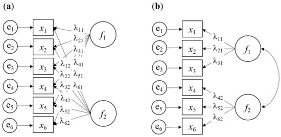
Figure 1.
Illustration of exploratory factor analysis (EFA) (a) and confirmatory factor analysis (CFA) (b) models with six observed variables (x1, …, x6), two latent variables (f1 and f2), and specific factors (e1, …, e6). Factor loadings are denoted by λ. Constraints on factor loadings or latent variances are omitted for simplicity.
This section provides a condensed overview of factor-model-parameter estimation methods, as detailed in Jöreskog [15] and Marôco [16]. Iterative techniques minimize a discrepancy function f (Equation (10)) using sample variance-covariance matrix (S) and expected covariance matrix ():
For maximum likelihood estimation (ML), under the normality assumption for the manifest variables, the discrepancy function to minimize is
Nonnormal data analysis recommends the asymptotic distribution free (ADF) [17] or weighted least squares (WLS) [18] estimators:
The generic element of W, calculated from the sample covariance elements and fourth-order moments of the observed x variables, is [19]:
The WLS estimator, considering sample covariances and fourth-order moments, may face convergence issues with small samples (<200). This problem can be addressed by diagonally weighted least squares (DWLS) or weighted least squares mean and variance (WLSMV) methods, both special cases of WLS. However, ignoring item covariances reduces statistical efficiency, impacting model fit. Ordinal factor analysis utilizes the polychoric correlation matrix, with the WLS estimator incorporating sample polychoric correlations (R) and thresholds to estimate the asymptotic covariance matrix (W). The discrepancy function, using observed (R)and estimated () polychoric correlations thus becomes [19,20]
1.2. Stanley Stevens and the Scales of Measurement
During the 1930s–40s, Stanley Stevens introduced a taxonomy for “scales of measurement,” influenced by the work of a committee from the British Association for the Advancement of Science [N. Campbell, p. 340 of the Final Report, cited in Stevens [21]]. Stevens proposed four scales: Nominal, Ordinal, Interval, and Ratio, which unified qualitative and quantitative measurements. Nominal scales evaluate attributes without magnitude, permitting only frequency and classification. Ordinal scales sort categories without quantifiable order, allowing classification and sorting operations. Interval scales record attributes with fixed intervals but lack an absolute zero, allowing distance comparison but not ratios. Ratio scales assess attributes with interpretable and comparable ratios. Stevens also outlined permissible central tendency and dispersion measures for each scale: nominal scales report modes; ordinal scales report modes, medians, and percentiles but not means or standard deviations; interval or ratio scales allow means, standard deviations, and correlation coefficients. Ratio-based statistics, like the coefficient of variation, are only admissible for ratio scales.
Is It Permissible to Do Factor Analysis with Ordinal Items?
Stevens’s taxonomy profoundly influenced the social sciences, particularly psychology, guiding statistical analysis for qualitative and quantitative variables. Many textbooks and statistical software rely on his taxonomy for recommendations on appropriate statistical analysis methods. However, criticisms of Stevens’s taxonomy have emerged [22,23]. Controversy remains regarding the treatment of variables measured on an ordinal scale [24]. Stevens recognizes that most scales used effectively by psychologists are ordinal scales, and thus, “In the strictest propriety the ordinary statistics involving means and standard deviations ought not to be used with these scales” ([21], p. 679). However, on the same page, Stevens recognizes that “On the other hand, for this ‘illegal’ statisticizing there can be invoked a kind of pragmatic sanction: In numerous instances, it leads to fruitful results”. Despite pragmatic justification for their use, some methodologists advocate against using such statistics for ordinal variables [9,25]. According to Stevens, only mode, median, and percentiles are permissible for ordinal variables. Prohibiting statistics like mean and correlation coefficients raises concerns for psychometry, where Likert items and factor analyses are prevalent. If statistics not permissible for ordinal scales are banned, could it compromise the validity of “correlational psychology” [18] and countless psychometric scales derived from ordinal measures through factor analysis on the Pearson correlation matrix? The validity of decades of psychometric research may be at risk?
2. Other Methods to Analyze Ordinal Items
Confirmatory factor analysis (CFA) emerged in the latter half of the 20th century, driven by the need to validate theoretical models across diverse populations empirically. Jöreskorg and Sörbom developed LisRel, the first commercial software for structural equation modeling, laying the groundwork for CFA. Babakus, Ferguson, & Jöreskog [26] conducted a seminal simulation study on CFA of ordinal items, finding that factor loadings estimated with polychoric correlations surpassed those obtained with Pearson’s, Spearman’s, and Kendall’s correlations. This study confirmed previous observations that Pearson correlations tend to underestimate factor loadings, particularly with ordinal items having fewer than five categories and considerable asymmetry. Independent simulation studies have corroborated these findings, noting that as the number of categories increases and distribution bias decreases, Pearson correlation estimates approach those of quantitative variables [8,27].
2.1. The Spearman Correlation Coefficient
Spearman developed his correlation coefficient as an alternative to Pearson’s, specifically for variables that could not be quantitatively measured [28]. Spearman’s rho, based on rank differences, is an adaptation of Pearson’s coefficient applied to the ranks (rx1i, rx2i) rather than the original observations (x1i, x2i) [28]:
2.2. The Polychoric Correlation Coefficient
The polychoric correlation coefficient, introduced by Karl Pearson in 1900, evaluates correlations between nonquantitatively measurable characteristics [29]. This coefficient gained attention in factor analysis after simulation studies demonstrated its superiority in estimating associations between ordinal items [6,20,26,30,31]. It assumes that qualitative characteristics on ordinal or nominal scales result from discretized continuous latent variables with bivariate normal distributions. Thus, the polychoric correlation coefficient estimates the linear association between two latent variables operationalized by ordinal variables (e.g., Likert-type items). For instance, an item with five categories, such as an agreement scale, is conceptualized as dividing a latent variable into categories defined by thresholds on the latent ξ:
The observed variable’s five response categories represent an approximation of the five intervals at which the latent continuous variable, denoted as ξ, has been divided using four cutoff points or thresholds: ξ1, ξ2, ξ3, and ξ4. Each of these k−1 thresholds can be determined based on the relative frequency of the k categories, assuming normality:
where Φ−1 is the inverse of the normal distribution, nk is the absolute frequency of the item’s k category, and N is the total of the item’s responses. By convention ξ0 = −∞ and ξ5 = +∞. The polychoric correlation coefficient is generally estimated by the maximum likelihood (see, e.g., Drasgow, 1986). In a two-step algorithm, the procedure begins by estimating the threshold for x1 and x2. If category i of variable x1 is observed when ξ1i−1 ≤ ξ1 < ξ1i and if category j of variable x2 is observed when ξ2j−1 ≤ ξ2 < ξ2j, then the joint probability (Pij) of observing the category x1i and x2j is:
where
is the bivariate normal density function of x1 and x2 with μ = 0 and σ = 1 (without loss of generality, since the original latent variables are origin- and scale-free), and Pearson correlation ρ. If nij is the number of observations x1i of X1 and x2j of X2, the sample likelihood is:
where k is a constant and u and v are the number of categories of X1 and X2, respectively. In the second step, the maximum likelihood estimates of the polychoric correlation coefficient (ρ) are obtained by deriving the Ln(L), with respect to ρ:
Equating the partial derivatives of Equation (20), with respect to all model parameters, to 0 and solving it with respect to ρ gives the polychoric correlation estimate [32]. The asymptotic covariance matrix of the estimated polychoric correlations can then be estimated using computational methods derived by Jöreskog [33] after Olsson [34]. The maximum likelihood solution is generally obtained iteratively in several commercial software (e.g., Mplus, LisRel, EQS) and free software (R psych and polycor packages) but not in IBM SPSS Statistics (up to version 29).
Simulation studies suggest that the polychoric correlation coefficient outperforms Pearson, Spearman, and Kendall correlations in reproducing the correlational structure of latent variables when operationalized as ordinal observed variables [26,31,35]. However, its usefulness as an alternative to the Pearson correlation coefficient is debated. For small samples (n < 300–500) with many variables, polychoric correlations may not yield better results than Pearson correlations [36]. Additionally, assumptions of bivariate normality and large sample sizes (>2000 observations) are needed for accurate estimation, posing challenges in practical structural equation modeling [17,37]. Moreover, the polychoric correlation lacks statistical robustness when the underlying distribution deviates strongly from bivariate normality, leading to potential inaccuracies in ordinal factor analysis [38,39]. It may also introduce bias when ordinal factor models impose a normality assumption for underlying continuous variables, which might also often be true in empirical applications [35,39,40].
This paper compares Pearson’s, Spearman’s, and Polychoric correlation coefficients using real and simulated data. It demonstrates calculating these coefficients using statistical software and applying the matrices in exploratory and confirmatory factor analysis (EFA and CFA). The findings are discussed regarding their implications for real data factor analysis applications.
3. Results
3.1. Case Study 1: Exploratory Factor Analysis of Ordinal Items with 3 Points
To demonstrate factor analysis with ordinal items, data from a study on voters’ perceptions [41] using a three-point ordinal scale is considered. Items include “People like me have no voice” (WithoutVoice), “Politics and government are too complex” (Complex), “Politicians are not interested in people like me” (Desinter), “Politicians once elected quickly lose contact with their voters” (Contact), and “Political parties are only interested in people’s votes” (Parties). Using IBM SPSS Statistics, classical EFA can be conducted on the covariance matrix or Pearson correlation matrix. Syntax for factor extraction using principal components with Varimax rotation on the correlation matrix is provided as Supplementary Material. Furthermore, EFA can be performed on the Spearman correlation matrix in SPSS Statistics. Syntax involves converting variables to ranks before conducting factor analysis (see Supplementary Material for syntax). Lastly, EFA on the polychoric correlations matrix is discussed. Since SPSS Statistics does not compute polychoric correlations, one can calculate and import the matrix from R using the polycor package [42]. Pearson, Spearman, and Polychoric correlation matrices for the five items are shown in Table 1.

Table 1.
Pearson’s (A) and Spearman’s (B) correlation matrices were obtained with SPSS Statistics, and the Polychoric correlation (C) matrix was obtained with the polycor (v. 0.7-9) package. All p-values for the bivariate normality tests were larger than 0.10.
With IBM SPSS Statistics, exploratory factor analysis (EFA) can now be conducted on the polychoric correlation matrix, along with other desired correlation matrices. Table 2 provides a summary of the relevant results from the three EFAs conducted on the Pearson, Spearman, and Polychoric correlation matrices. Factors were extracted using Kaiser’s criterion (eigenvalue greater than 1).
Table 2.
Summary of the results of the exploratory factor analyses with the extraction of principal components with varimax rotation performed on the Pearson, Spearman, and Polychoric correlation matrices.
The variance extracted by each of the two retained factors is higher in the analysis conducted on the polychoric correlation matrix compared to the analyses on the Pearson or Spearman correlation matrices (59.9% vs. 53.3% vs. 51.7%, respectively, for the first factor F1; the differences for the second factor F2 are even smaller). Similarly, the factor loadings for each factor are higher when using the polychoric correlations, followed by Pearson’s and then Spearman’s correlations. These differences, often to the second decimal place, are visually depicted in Figure 2, highlighting their significance.
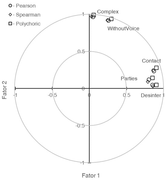
Figure 2.
Graphical representation of the two extracted factor loadings on Complex, WithoutVoice, Contact, Departures, and Desinter with exploratory factor analysis on Pearson’s ( ), Spearman’s (
 ) and the polychoric (
 ) correlation matrices.
), Spearman’s () and the polychoric () correlation matrices.
3.2. Case Study 2: Confirmatory Factor Analysis of Ordinal Items with 5 Points
Case study 2 involves confirmatory factor analysis (CFA) of the USEI, a psychometric inventory assessing academic engagement. Comprising 15 ordinal items, the USEI’s response categories range from “1-Never” to “5-Always”. It conceptualizes academic involvement as a second-order hierarchical structure, with three first-order factors: Behavioral, Emotional, and Cognitive engagement, each consisting of five ordinal items [43]. Although most items exhibit slight leftward skewness, observed skewness (sk) and excess kurtosis (ku) values, do not indicate severe departures from normal distribution [16].
Using the R software and the lavaan package [44], CFA can be conducted employing various correlation matrices and appropriate estimators based on the measurement scales of observed variables. The recommended estimators include maximum likelihood for normally distributed, at least interval-scale items; or WLSMV/DWLS for ordinal items with underlying bivariate normal latent variables [30]. Traditional CFA, utilizing the covariance matrix and maximum likelihood estimation of the model described in Equation (11), can be executed with the lavaan library in R using the Pearson correlation matrix (see Supplementary Material for R code). To perform CFA on the polychoric correlation matrix, ordinal item specification with the ordered keyword is necessary (by default, lavaan utilizes the DWLS estimator). Table 3 summarizes the primary outcomes of these two analyses. Both models exhibit good fit, whether using the traditional method (maximum likelihood on the covariance matrix) or the more recent method (DWLS on the polychoric correlation matrix). All items display standardized factor loadings exceeding the typical cutoff value in factor analysis (λ ≥ 0.5). Differences in factor loading estimates are minimal, mostly favoring the DWLS method on the polychoric correlation matrix.
Table 3.
Standardized factor weights (λ) for the USEI second-order hierarchical model estimated with the MLE method on the Pearson correlation matrix (χ2(87) = 241.22, CFI = 0.945, TLI = 0.933, RMSEA = 0.054 with IC90% ]0.046; 0.062[) vs. DWLS method on the matrix of polychoric correlations (χ2(87) = 172.249, CFI = 0.994, TLI = 0.993, rmsea = 0.040 with IC90% ]0.031; 0.049[) using the lavaan package.
3.3. Case Study 3: Confirmatory Factor Analysis of Ordinal Items—Artificial Results?
The case studies thus far suggest an advantage in conducting either exploratory or confirmatory factor analysis of ordinal items using the polychoric correlation matrix over Pearson’s correlation. However, it is crucial to note that the observed differences in standardized factor loadings between the two methods are typically minimal, only affecting the second decimal place of estimates, and do not significantly alter the researcher’s conclusions regarding the underlying factor structure. Additionally, as highlighted by Finney et al. [19], while the results with MLE and DWLS estimators are promising, there remains uncertainty about their performance with ordinal items exhibiting varying numbers of categories and distributions.
To further illustrate this uncertainty, a case study of the Postpartum Bonding Questionnaire (PBQ) with 25 ordinal items and six categories each is presented [45]. Descriptive statistics for the PBQ items are provided (see Supplementary Material). Employing the lavaan package, CFA was conducted on both the Pearson correlation matrix with MLE and the Polychoric correlation matrix with DWLS estimation. The results, summarized in Table 4, indicate notable differences favoring the analysis of the polychoric correlation matrix with DWLS.
Table 4.
Standardized factor weights (λ) for the tetrafactorial model of the PBQ estimated with the maximum likelihood (MLE) method on the Pearson correlation matrix (χ2(269) = 2838.41, CFI = 0.670, TLI = 0.632, RMSEA = 0.067 with IC90% ]0.064; 0.069[) and with DWLS method on the matrix of polychoric correlations (χ2(87) = 172.249, CFI = 0.994, TLI = 0.993, rmsea = 0.040 with IC90% ]0.031; 0.049[) using the lavaan package.
In this case study, contrary to the previous ones, the differences in standardized factor loadings, extending to the first decimal place, significantly favor the analysis of the polychoric correlation matrix with DWLS. While MLE analysis on the covariance matrix yields standardized weights mostly below 0.5, DWLS analysis on the polychoric correlation matrix results in higher factor loadings. Consequently, the goodness of fit for the tetra-factorial model obtained with DWLS on the polychoric correlation matrix is substantially better than that obtained with MLE on the Pearson covariance matrix. Specifically, using DWLS on the polychoric correlation matrix, the model fit is deemed good, whereas MLE on the covariance matrix yields a relatively poor fit.
The apparent superiority of CFA estimates derived from polychoric correlations compared to those from Pearson’s covariance/correlation matrix is evident. However, the reliability of these polychoric correlation-based estimates relative to those from the Pearson correlation matrix warrants scrutiny. Particularly in case study 3, where items exhibit significant asymmetry, it raises questions about the accuracy of these estimates.
To address this, a simulation study using various levels of skewness and excess kurtosis for five-point ordinal variables with known factor structures can provide valuable insights. By comparing the performance of CFA estimates derived from polychoric correlations with those from Pearson’s correlation matrix under different data conditions, we can evaluate the robustness and reliability of the former approach.
4. Simulation Studies
Let us consider a two-factor population model with three items each (see Supplementary Material), where the standardized factor loadings are 0.5, 0.6, and 0.7 for each item and a correlation of 0.5 between the two factors. Using the lavaan package’s simulateData function with model.type = “cfa”, I generated one million standardized data observations with skewness and excess kurtosis values of 0. The descriptive statistics and correlations of the generated items are shown in Figure 3A, indicating normal distribution with small to moderate observed Pearson correlations between the items.
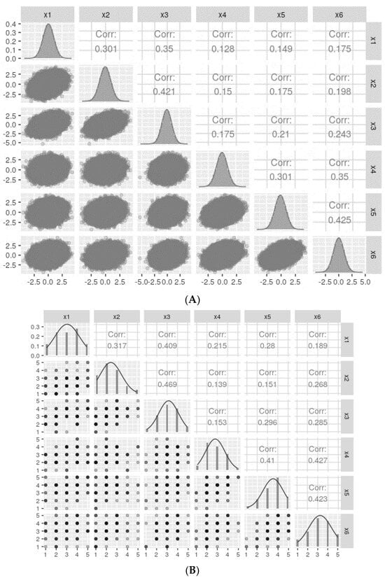
Figure 3.
Data distribution for continuous (A) and categorized (B) variables was generated with the model described in 4. Simulation studies For simplicity, only the ncat = 5 category variables are presented. Note that for normally distributed data, Pearson correlations are similar for both continuous and five-categories categorized variables.
Assuming the ordinal items result from discretizing latent continuous variables into a given number of categories (ncat = 5, 7, and 9), the continuous variables generated previously can be discretized accordingly. The categorized data is depicted in Figure 3B.
Subsequent simulations were conducted under two scenarios: (i) Symmetrical (normal) ordinal variables with 5, 7, and 9 categories; (ii) Biased (non-symmetrical) ordinal data generated from biased continuous variables; and (iii) Biased (nonsymmetrical) variables obtained by biased sampling from ordinal symmetrical variables.
4.1. Simulation 1: Symmetrical Ordinal Data Generated from Normal Continuous Data
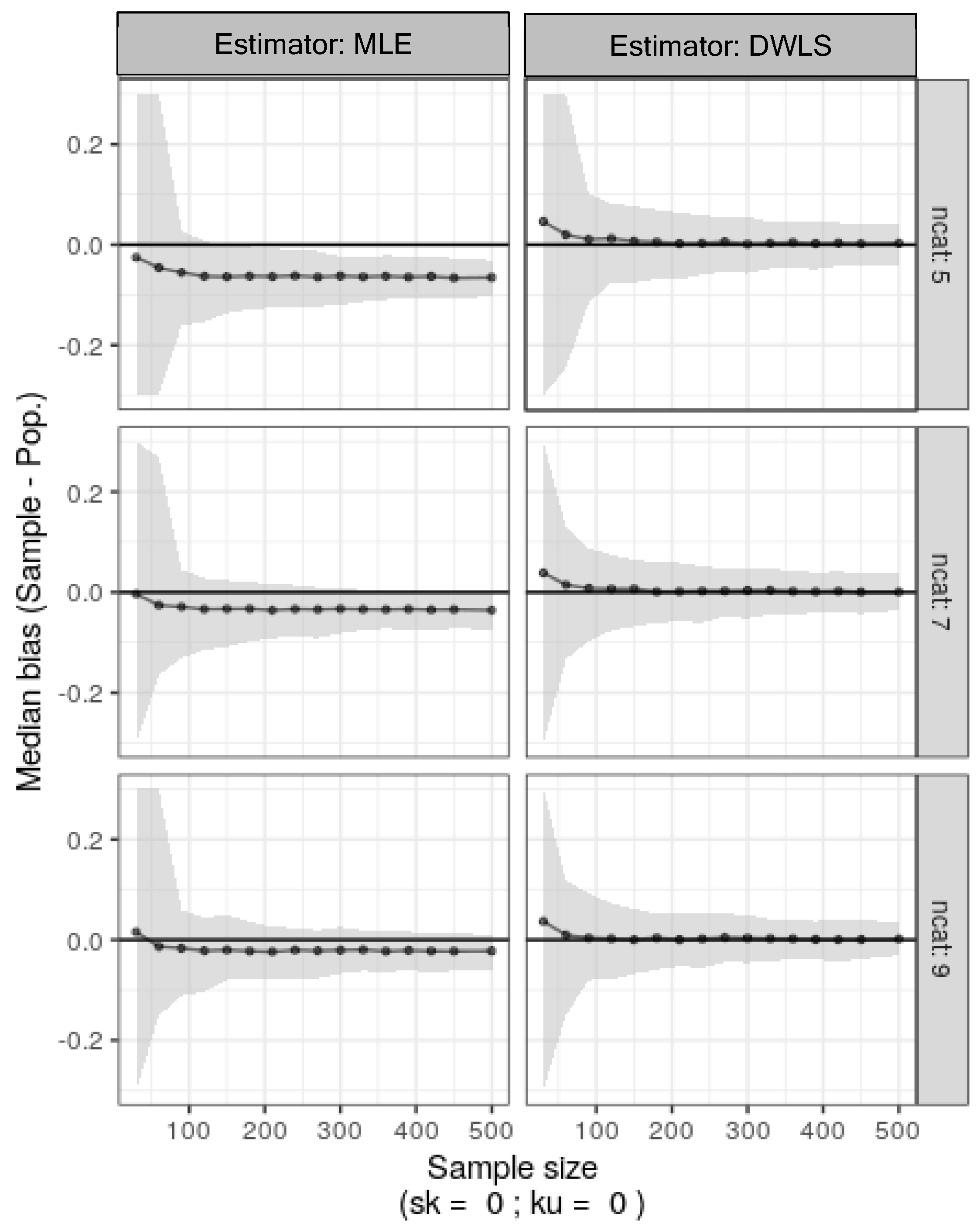
A model was created with R-lavaan to fit the two-factor population data. It was then applied using DWLS or MLE to data sampled with replacement from the original ordinal generated data with sample sizes ranging from 30 to 500 and 500 bootstrap replicates. Results in Figure 4 show that MLE on Pearson correlations for ordinal items consistently underestimated true population factor loadings. This underestimation increased with fewer categories (from 9 to 5). Conversely, DWLS estimation quickly converged to true population factor loadings, unaffected by the number of categories, even for small sample sizes.

Figure 4.
Median bias estimates for factor loadings and nonparametric 95% confidence intervals (shaded area) were calculated as the percentiles 2.5 and 97.5 from 500 bootstrap samples from the original symmetrical ordinal generated data. This was done with different numbers of categories (ncat: 5, 7, or 9) and sample sizes ranging from 30 to 500.
4.2. Simulation 2: Symmetrical Ordinal Data Generated from Nonnormal Continuous Data
Simulation two mirrored simulation one, except the original data was skewed and leptokurtic (sk = −3, ku = 7). Results from 500 bootstrap replicates are shown in Figure 5. MLE and DWLS yielded biased estimates, with MLE notably poor for five-category ordinal variables. DWLS showed resilience to category count, converging even with small sample sizes in SEM (n = 100–150), albeit with noticeable bias.
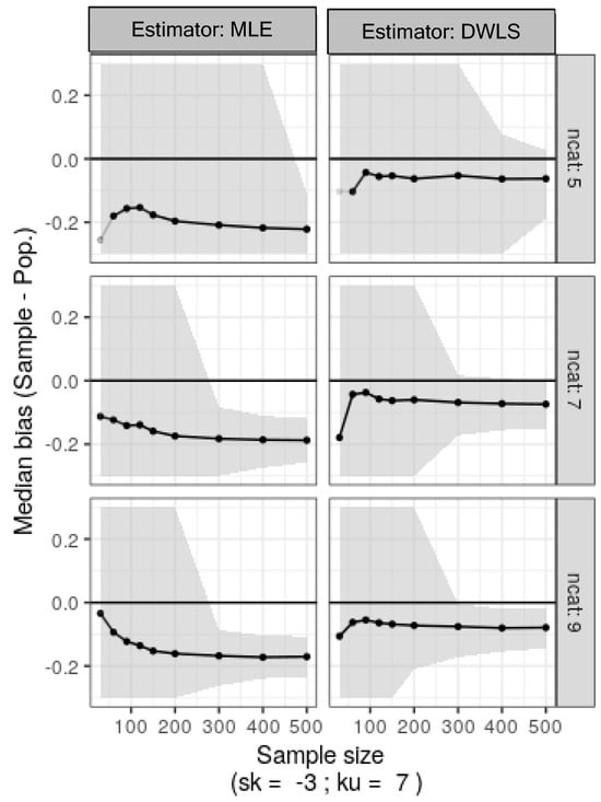
Figure 5.
Median bias estimates for factor loadings and nonparametric 95% confidence intervals (shaded) calculated as the percentiles 2.5 and 97.5 from 500 bootstrap samples of the original skewed ordinal data with varying category counts (ncat: 5, 7, or 9) and sample sizes (30 to 500).
4.3. Simulation 3: Asymmetrical Ordinal Data Generated from Biased Sampling of Normal Ordinal Data
Simulation three explores biased responses stemming from nonrandom sampling practices prevalent in psychological and social sciences research. Despite the fact that a normative population exhibits a normal distribution, nonrandom sampling and respondent bias lead to highly asymmetrical data. Only biased responses from the original population (N = 106) were sampled. As shown in Figure 6, with data from biased items featuring seven categories, MLE consistently underestimates the true population factor loadings. Surprisingly, DWLS exhibits an opposite trend, overestimating the true population factor loadings. This contrasts with the asymmetrical data generated in simulation 2.
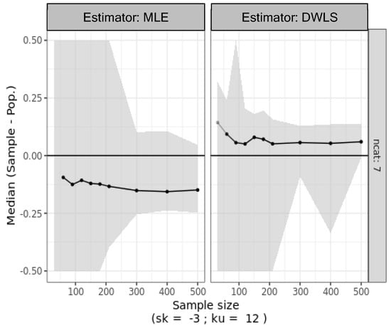
Figure 6.
Median bias in factor loading estimates and nonparametric 95% confidence intervals (shaded area) calculated as the percentiles 2.5 and 97.5 from 500 bootstrap samples of the biased ordinal data with seven categories and varying sample sizes (30 to 500).
5. Discussion
The simulation and case studies conducted demonstrate that polychoric correlation coefficients tend to be higher than Pearson’s and Spearman’s coefficients, indicating their robustness in estimating latent variables. Polychoric correlations, which are derived from the assumption of normally distributed latent variables, are generally less susceptible to measurement errors associated with ordinal data. This characteristic leads to factor loadings extracted from the polychoric correlation matrix being higher, thus supporting consistent theoretical interpretations, even with small sample sizes. This robustness makes polychoric correlations particularly valuable in psychometrics, where latent constructs are often measured using ordinal scales.
However, the exclusive reliance on polychoric correlations and weighted least squares (WLS) methods for factor analysis with ordinal variables—especially those with few categories—may not always be justifiable. Recent studies have explored the limitations of these methods, particularly in conditions where the assumptions underlying polychoric correlations (e.g., normality of latent variables) are violated. For instance, simulation studies by Flora and Curran [46] have shown that polychoric correlations are robust to modest violations of underlying normality and that WLS performed adequately only at the largest sample size but led to substantial estimation difficulties with smaller samples. However, Li [6,18] showed that WLSMV yielded moderate overestimation of interfactor correlations when the sample size was small or/and when the latent distributions were moderately nonnormal and that factor models tended to be overrejected by chi-square statistics with bot estimators for small sample sizes (n = 200). Combined, these studies show that WLS on polychoric correlations may overestimate factor loadings when data are strongly skewed or when the assumption of multivariate normality is not met. This overestimation can lead to inflated perceptions of model fit and factor validity.
In case studies 1 and 2, Pearson’s maximum likelihood estimation (MLE) and polychoric correlations with diagonally weighted least squares (DWLS) estimation produced similar results, with negligible differences in standardized factor loadings. This consistency supports the validity of factor interpretations under these conditions, aligning with findings from studies like those by Robitzsch [39]. who noted that under moderate data conditions, the differences between Pearson correlations and polychoric correlations are often minimal. This suggests that, in such cases, either method could be appropriately used without significantly impacting the outcomes of the factor analysis.
However, case study 3 revealed substantial disparities between the estimates obtained from Pearson correlations with MLE and polychoric correlations with DWLS estimation. The latter yielded substantially higher factor loadings, which led to conflicting conclusions regarding factorial validity. This discrepancy underscores the potential risks associated with relying solely on polychoric correlations, especially in cases where data may be biased or the assumptions of the polychoric model are not fully met. A similar issue was highlighted by Robitzsch [40], who cautioned against overreliance on polychoric correlations, noting that their application in the presence of model misspecification can lead to misleading interpretations of factor structures.
Moreover, simulation study 3 highlighted the unreliability of polychoric correlations with DWLS under biased data conditions. While MLE on Pearson correlations consistently underestimated true population parameters, DWLS on polychoric correlations tended to overestimate them, a phenomenon particularly evident in scenarios involving biased or nonnormal data. This aligns with findings from Flora and Curran [46], who reported that the inadequacy of least squares weighted methods with polychoric correlation matrices becomes particularly pronounced under conditions of severe non-normality. These authors demonstrated that under such conditions, WLS methods could yield highly biased parameter estimates, calling into question the reliability of conclusions drawn from such analyses.
Additionally, methodological recommendations often suggest selecting estimation techniques based on the number of categories in the data. For example, Rhemtulla, Brosseau-Liard, and Savalei [8] recommended using WLS for data with fewer categories, while MLE might be more appropriate for data with more categories. However, our findings suggest that these methodological differences are relatively minor under typical data conditions but become significant under strongly data biased scenarios. This is consistent with our real data and simulation results, emphasizing the importance of considering the specific characteristics of the data when choosing between estimation methods, warning that blind reliance on polychoric correlations with weighted least squares estimates could lead to misleading conclusions about factor structure validity and reliability.
6. Concluding Remarks
While polychoric correlations and DWLS can be powerful tools in factor analysis, especially with ordinal data, their use must be carefully considered in light of the data distributional characteristics. The evidence suggests that in situations involving data nonnormality or other biases, these methods may not be the most reliable, and alternative approaches, such as robust maximum likelihood or Bayesian methods, may offer more accurate results. Method selection should consider data characteristics, with distributional analyses imperative, especially under biased conditions. These findings contribute to ongoing discussions about the appropriate use of correlation matrices and estimation methods in factor analysis.
Supplementary Materials
The following supporting information can be downloaded at https://www.mdpi.com/article/10.3390/stats7030060/s1.
Funding
This research received no external funding.
Institutional Review Board Statement
Not applicable.
Informed Consent Statement
Not applicable.
Data Availability Statement
See Supplementary Material for data and code.
Conflicts of Interest
The author declares no conflict of interests.
References
- Spearman, C. General Intelligence, Objectively Determined and Measured. Am. J. Psychol. 1904, 15, 201. [Google Scholar] [CrossRef]
- Thomson, G.H. A Hierarchy Without a General Factor. Br. J. Psychol. 1916, 8, 271–281. [Google Scholar] [CrossRef]
- Thurstone, L.L. Primary Mental Abilities; University of Chicago Press: Chicago, IL, USA, 1938; Available online: http://catalog.hathitrust.org/api/volumes/oclc/2471740.html (accessed on 1 August 2024).
- Likert, R. A Technique for the Measurement of Attitudes. Arch. Psychol. 1932, 22, 55. [Google Scholar]
- Muthén, B.; Kaplan, D. A comparison of some methodologies for the factor analysis of non-normal Likert variables. Br. J. Math. Stat. Psychol. 1985, 38, 171–189. [Google Scholar] [CrossRef]
- Li, C.H. The performance of ML, DWLS, and ULS estimation with robust corrections in structural equation models with ordinal variables. Psychol. Methods 2016, 21, 369–387. [Google Scholar] [CrossRef] [PubMed]
- Li, C.H. Confirmatory factor analysis with ordinal data: Comparing robust maximum likelihood and diagonally weighted least squares. Behav. Res. 2015, 48, 936–949. [Google Scholar] [CrossRef]
- Rhemtulla, M.; Brosseau-Liard, P.É.; Savalei, V. When can categorical variables be treated as continuous? A comparison of robust continuous and categorical SEM estimation methods under suboptimal conditions. Psychol. Methods 2012, 17, 354–373. [Google Scholar] [CrossRef]
- Liddell, T.M.; Kruschke, J.K. Analyzing ordinal data with metric models: What could possibly go wrong? J. Exp. Soc. Psychol. 2018, 79, 328–348. [Google Scholar] [CrossRef]
- Foldnes, N.; Grønneberg, S. Pernicious Polychorics: The Impact and Detection of Underlying Non-normality. Struct. Equ. Model. 2020, 27, 525–543. [Google Scholar] [CrossRef]
- Cattell, R.B. The measurement of adult intelligence. Psychol. Bull. 1943, 40, 153–193. [Google Scholar] [CrossRef]
- Bartholomew, D.J. Three Faces of Factor Analysis. In Factor Analysis at 100: Historical Developments and Future Directions; Lawrence Erlbaum Associates Publishers: Mahwah, NJ, USA, 2007; pp. 9–21. [Google Scholar]
- de Winter, J.C.F.; Dodou, D. Factor Recovery by Principal Axis Factoring and Maximum Likelihood Factor Analysis as a Function of Factor Pattern and Sample Size. J. Appl. Stat. 2011, 39, 695–710. [Google Scholar] [CrossRef]
- Lawley, D.N.; Maxwell, A.E. Factor Analysis as a Statistical Method. Stat 1962, 12, 209. [Google Scholar] [CrossRef]
- Jöreskog, K.G. Factor Analysis and Its Extensions. In Factor Analysis at 100: Historical Developments and Future Directions; Lawrence Erlbaum Associates Publishers: Mahwah, NJ, USA, 2007; pp. 47–77. [Google Scholar]
- Marôco, J. Análise de Equações Estruturais: Fundamentos Teóricos, Software & Aplicações, 3rd ed.; ReportNumber: Pêro Pinheiro, Portugal, 2014; ISBN 9789899676367. [Google Scholar]
- Arbuckle, J. Amos, Version 4.0. [Computer Software]; SPSS: Chicago, IL, USA, 2006.
- Li, C.-H. The Performance of MLR, USLMV, and WLSMV Estimation in Structural Regression Models with Ordinal Variables. J. Chem. Inf. Model. 2014, 53, 1689–1699. [Google Scholar] [CrossRef]
- Finney, S.J.; DiStefano, C. Nonnormal and Categorical Data in Structural Equation Modeling. In A Second Course in Structural Equation Modeling, 2nd ed.; Hancock, G.R., Mueller, R.O., Eds.; Information Age: Charlotte, NC, USA, 2013. [Google Scholar]
- Muthén, B. A general structural equation model with dichotomous, ordered categorical, and continuous latent variable indicators. Psychometrika 1984, 49, 115–132. [Google Scholar] [CrossRef]
- Stevens, S.S. On the theory of scales of measurement. Science 1946, 103, 677–680. [Google Scholar] [CrossRef]
- Lord, F.M. On the statistical treatment of football numbers. Am. Psychol. 1953, 8, 750–751. [Google Scholar] [CrossRef]
- Velleman, P.F.; Wilkinson, L. Nominal, ordinal, interval, and ratio typologies are misleading. Am. Stat. 1993, 47, 65–72. [Google Scholar] [CrossRef]
- Feuerstahler, L. Scale Type Revisited: Some Misconceptions, Misinterpretations, and Recommendations. Psych 2023, 5, 234–248. [Google Scholar] [CrossRef]
- Jamieson, S. Likert scales: How to (ab)use them. Med. Educ. 2004, 38, 1217–1218. [Google Scholar] [CrossRef]
- Babakus, E.; Ferguson, C.E.; Joreskog, K.G. The Sensitivity of Confirmatory Maximum Likelihood Factor Analysis to Violations of Measurement Scale and Distributional Assumptions. J. Mark. Res. 1987, 24, 222–228. [Google Scholar] [CrossRef]
- Bollen, K.A. Structural Equations with Latent Variables; John Wiley & Sons: Hoboken, NJ, USA, 1989. [Google Scholar]
- Spearman, C. The Proof and Measurement of Association between Two Things. Am. J. Psychol. 1904, 15, 72. [Google Scholar] [CrossRef]
- Pearson, K. Mathematical Contributions to the Theory of Evolution. VII. On the Correlation of Characters Not Quantitatively Measurable. Philos. Trans. R. Soc. Lond. Ser. A Math. Phys. Eng. Sci. 1900, 195, 1–47. [Google Scholar]
- Finney, S.J.; DiStefano, C.; Kopp, J.P. Overview of estimation methods and preconditions for their application with structural equation modeling. In Principles and Methods of Test Construction: Standards and Recent Advances; Schweizer, E.K., DiStefano, C., Eds.; Hogrefe Publishing: Boston, MA, USA, 2016; pp. 135–165. ISBN 9780889374492. [Google Scholar]
- Holgado-Tello, F.P.; Chacón-Moscoso, S.; Barbero-García, I.; Vila-Abad, E. Polychoric versus Pearson correlations in exploratory and confirmatory factor analysis of ordinal variables. Qual. Quant. 2009, 44, 153–166. [Google Scholar] [CrossRef]
- Drasgow, F. Polychoric and Polyserial Correlations. In Encyclopedia of Statistical Sciences; Samuel, E.K., Balakrishnan, N., Read, C.B., Vidakovic, B., Johnson, N.L., Eds.; John Wiley & Sons: Hoboken, NJ, USA, 1986; pp. 68–74. [Google Scholar]
- Jöreskog, K.G. On the estimation of polychoric correlations and their asymptotic covariance matrix. Psychometrika 1994, 59, 381–389. [Google Scholar] [CrossRef]
- Olsson, U. Maximum likelihood estimation of the polychoric correlation coefficient. Psychometrika 1979, 44, 443–460. [Google Scholar] [CrossRef]
- Grønneberg, S.; Foldnes, N. Factor Analyzing Ordinal Items Requires Substantive Knowledge of Response Marginals. Psychol. Methods 2024, 29, 65–87. [Google Scholar] [CrossRef]
- Rigdon, E.E.; Ferguson, C.E. The Performance of the Polychoric Correlation Coefficient and Selected Fitting Functions in Confirmatory Factor Analysis with Ordinal Data. J. Mark. Res. 2006, 28, 491. [Google Scholar] [CrossRef]
- Yung, Y.-F.; Bentler, P.M. Bootstrap-corrected ADF test statistics in covariance structure analysis. Br. J. Math. Stat. Psychol. 1994, 47, 63–84. [Google Scholar] [CrossRef]
- Ekström, J. A Generalized Definition of the Polychoric Correlation Coefficient; Department of Statistics, UCLA: Los Angeles, CA, USA, 2011; pp. 1–24. [Google Scholar]
- Robitzsch, A.A. Why Ordinal Variables Can (Almost) Always Be Treated as Continuous Variables: Clarifying Assumptions of Robust Continuous and Ordinal Factor Analysis Estimation Methods. Front. Educ. 2020, 5, 177. [Google Scholar] [CrossRef]
- Robitzsch, A.A. On the Bias in Confirmatory Factor Analysis When Treating Discrete Variables as Ordinal Instead of Continuous. Axioms 2022, 11, 162. [Google Scholar] [CrossRef]
- Marôco, J.P. Statistical Analysis with SPSS Statistics, 8th ed.; ReportNumber: Pêro Pinheiro, Portugal, 2021; ISBN 978-989-96763-7-4. [Google Scholar]
- Fox, J. Polycor: Polychoric and Polyserial Correlations. R Package Version 0.7-9. 2016. Available online: https://cran.r-project.org/package=polycor (accessed on 1 August 2024).
- Maroco, J.; Maroco, A.L.; Bonini Campos, J.A.D.; Fredricks, J.A. University student’s engagement: Development of the University Student Engagement Inventory (USEI). Psicol. Reflex. E Crit. 2016, 29, 21. [Google Scholar] [CrossRef]
- Rosseel, Y. Lavaan: An R package for structural equation modeling. J. Stat. Softw. 2012, 48, 1–21. [Google Scholar] [CrossRef]
- Saur, A.M.; Sinval, J.; Marôco, J.P.; Bettiol, H. Psychometric Properties of the Postpartum Bonding Questionnaire for Brazil: Preliminary Data. In Proceedings of the 10th International Test Comission Conference, Vancouver, BC, Canada, 1–4 July 2016. [Google Scholar]
- Flora, D.B.; Curran, P.J. An Empirical Evaluation of Alternative Methods of Estimation for Confirmatory Factor Analysis with Ordinal Data. Psychol. Methods 2004, 9, 466–491. [Google Scholar] [CrossRef]


Disclaimer/Publisher’s Note: The statements, opinions and data contained in all publications are solely those of the individual author(s) and contributor(s) and not of MDPI and/or the editor(s). MDPI and/or the editor(s) disclaim responsibility for any injury to people or property resulting from any ideas, methods, instructions or products referred to in the content. |
© 2024 by the author. Licensee MDPI, Basel, Switzerland. This article is an open access article distributed under the terms and conditions of the Creative Commons Attribution (CC BY) license (https://creativecommons.org/licenses/by/4.0/).