Article

Examining Factors That Affect Movie Gross Using Gaussian Copula Marginal Regression

1
Computer Science Discipline, Division of Science and Mathematics, University of Minnesota-Morris, Morris, MN 56267, USA
2
Statistics Discipline, Division of Science and Mathematics, University of Minnesota-Morris, Morris, MN 56267, USA
*
Author to whom correspondence should be addressed.
Forecasting 2022, 4(3), 685-698; https://doi.org/10.3390/forecast4030037
Submission received: 18 May 2022 / Revised: 8 July 2022 / Accepted: 19 July 2022 / Published: 21 July 2022

Abstract

:
In this research, we investigate the relationship between a movie’s gross and its budget, year of release, season of release, genre, and rating. The movie data used in this research are severely skewed to the right, resulting in the problems of nonlinearity, non-normal distribution, and non-constant variance of the error terms. To overcome these difficulties, we employ a Gaussian copula marginal regression (GCMR) model after adjusting the gross and budget variables for inflation using a consumer price index. An analysis of the data found that year of release, budget, season of release, genre, and rating were all statistically significant predictors of movie gross. Specifically, one unit increases in budget and year were associated with an increase in movie gross. G movies were found to gross more than all other kinds of movies (PG, PG-13, R, and Other). Movies released in the fall were found to gross the least compared to the other three seasons. Finally, action movies were found to gross more than biography, comedy, crime, and other movie genres, but gross less than adventure, animation, drama, fantasy, horror, and mystery movies.

1. Introduction

The COVID-19 pandemic has negatively impacted the movie theater industry, but online movie-streaming businesses, such as Netflix, have been successful over this pandemic period. Because movies are now a significant part of culture in societies across the world and are a source of entertainment, the movie industry has become increasingly popular. The rise of the movie industry is highlighted by pop culture hits such as Star Wars and the Marvel Cinematic Universe (MCU). Movies such as these have become must-see worldwide phenomena, as indicated by the MCU and Star Wars movies occupying 5 of the 10 highest grossing movies of all time slots [1]. The movie industry as a whole has also been experiencing a high amount of success. In 2018, the Motion Picture Association of America reported that worldwide ticket sales hit a record USD 41.1 billion [2]. Although the movie industry has been experiencing an unprecedented amount of success, not all movies are guaranteed to be box office hits. There are films such as Avengers: Endgame that make eight times their budget, movies like The Shawshank Redemption which make a minimal profit (grossed 28 million with a budget of 25 million), and then there are movies that lose money such as Hot Tub Time Machine 2 (grossed 13.1 million with a budget of 14 million). Budgets, among many other conjectured factors, played a significant role in the performance of successful movies in the U.S. [3].
Given that not all movies share an equal amount of success, researchers have predicted movie performance using linear regression, logistic regression, and machine learning. A decision support system to help movie investment decisions at the early stages of movie productions was created by using social network analysis and a text mining technique [4]. The possibility that an individual-level decrease in preference over time is the cause of the decline in revenue that many movies experience after opening was investigated in [5]. Machine learning is a well-employed method and has been used to build prediction models in [6,7]. An ensemble approach for predicting box office performance was used in [7], and machine learning for the prediction of the box office was considered in [8]. Text mining and exploratory factor analysis to examine the relationship between a movie’s success and its title in China and United States was done in [9]. Part of their analysis found that sequel movies that have titles similar to their predecessor were more likely to be successful [9]. Machine learning methods for predicting movie performance were considered in [10], and social network analysis and text mining methods for Hollywood movie analysis were used in [11].
Copula does not need any assumptions such as independence, linearity, or normality of residuals (see references [12,13,14]). The reason to use a Gaussian copula marginal regression (GCMR) model [15] in this paper is that GCMR models do not require that the residuals be normally distributed or be evenly distributed around zero. Additionally, GCMR models include a dispersion parameter that is able to model and adjust for non-constant variance. The GCMR model is frequently used in the analysis of financial data [16,17]. The GCMR method to find high dependence between the exchange rates and daily crude oil prices was considered in [18]. A multiple linear regression model made to measure the relationship between callable and non-callable corporate bond yields and explanatory variables such as liquidity and coupon rate experienced the problems of heteroscedasticity and the non-normal distribution of the residuals [19]. To avoid the problems caused by using multiple linear regression with the movie data, we propose using a copula method (GCMR) to analyze the data.
The remainder of this paper is organized as follows: Section 2 provides a description of the data, Section 3 describes the statistical methods used to analyze the data, which includes multiple linear regression and GCMR, Section 4 summarizes the findings of the data analysis, and Section 5 presents our conclusions.

2. Data Description

The goal of this study is to answer questions regarding the movie industry, specifically the relationship between a movie’s gross and several other factors. The hypothesis that we consider in this research is that there is a relationship between a movie’s gross and its budget, season of release, year of release, rating, and genre. To investigate our hypothesis that a movie’s budget, season of release, year of release, rating, and genre affect the amount it grosses, we downloaded a dataset from Kaggle.com. Kaggle is a website on which users can upload datasets for others to use. The dataset used for this study was uploaded by Daniel Grijalva and can be found here https://www.kaggle.com/datasets/danielgrijalvas/movies, accessed on 5 February 2022. The dataset contains information about movies pulled from IMDb. To construct the dataset, Grijalva used a python script and IMDb’s advanced search tool to gather information about the most popular movies throughout the years. The dataset contains information for 7668 movies ranging from 1980 to 2020. The dataset contains fifteen variables: name, rating, genre, year, released, score, votes, director, writer, star, country, budget, gross, company, and runtime. For this study, the primary variables of interest are:
  • rating: categorical variable with the levels of G, PG, PG-13, R, NC-17, TV-PG, TV-14, TV-MA, Not Rated, Unrated, X, and Approved
  • genre: categorical variable with levels of drama, adventure, action, comedy, horror, biography, crime, fantasy, family, sci-fi, animation, romance, music, western, thriller, history, mystery, sport, and musical
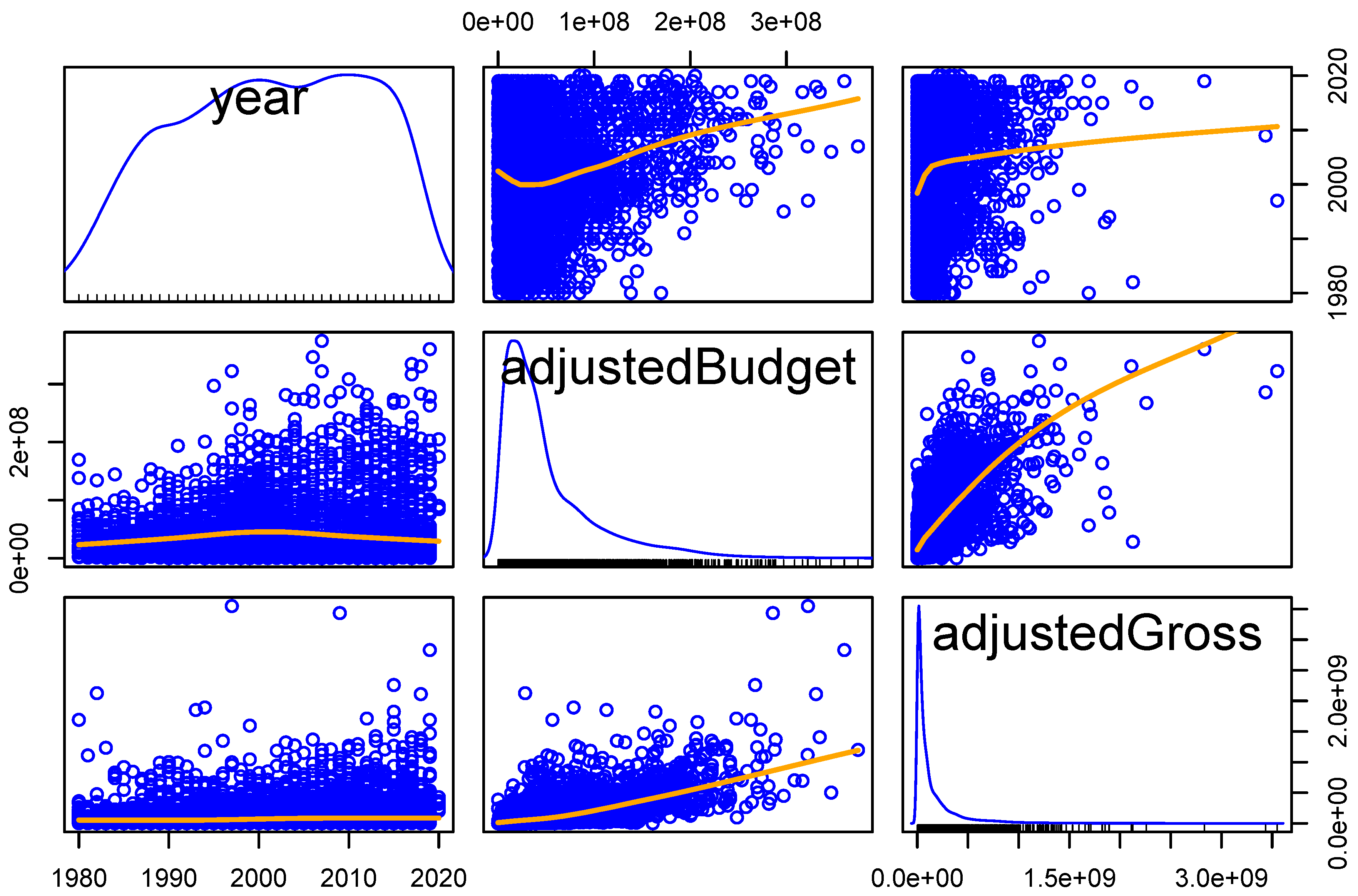
  • year: numerical variable with values ranging from 1980 to 2020
  • released: character variable formatted as “Month Day, Year”
  • budget: numerical variable measured in United States dollar
  • gross: numerical variable measured in United States dollar. Additionally, this refers to U.S. gross only
An extensive amount of data cleaning had to be performed to get the data ready for analysis. First, it is important to note that IMDb does not adjust for inflation in their calculations of a movie’s gross and budget. This is problematic, as the dataset contains movies dating back to 1980. As such, in order to ensure we would be accurately describing the relationship between a movie’s gross and its budget, genre, year, season, and rating, we adjusted the gross and budget variables for inflation. To adjust the gross and budget variables for inflation, we downloaded a consumer price index (CPI) table from the Federal Reserve Bank of Minneapolis website, which can be found here: https://www.minneapolisfed.org/about-us/monetary-policy/inflation-calculator/consumer-price-index-1913-, accessed on 19 March 2022. The table contains a column for the year, a column for the annual average CPI(-U), and a column for the annual percent change (rate of inflation). The CPI(-U) means that we are using the CPI value associated with the changes in prices paid by urban consumers. The equation to adjust for inflation is as follows:
Year   2   Price = Year   1   Price × Year   2   CPI Year   1   CPI .
Two datasets (the movies dataset and the CPI) were merged by using the sqldf R package. The new dataset contained a new variable called CPI. The value of the CPI variable was the correct CPI value for the year that each movie was released. For example, a movie released in 1980 had a CPI value of 82.4, and a movie released in 2010 had a CPI value of 218.1. New inflation-adjusted versions of the gross and budget variables were created called adjustedGross and adjustedBudget. The dollar amounts were adjusted to the latest year in the dataset, which was 2020. As such, the formula to calculate adjustedGross was:
Year   2020   Gross = G r o s s x × Year   2020   CPI C P I x
where x is the movie that we are performing the calculation on. The formula for adjustedBudget was similar, except instead of calculating the 2020 gross we were calculating the 2020 budget:
Year   2020   Budget = B u d g e t x × Year   2020   CPI C P I x .
After the creation of the inflation-adjusted variables, the dataset was then filtered to only movies made within the United States, bringing the number of observations down to 5475. The observations with missing values related to the variables of interest (rating, budget/adjustedBudget, and gross/adjustedGross) were then dropped. This brought down the number of observations from 5475 to 4322. After dropping the NA values, a new categorical variable called season was created from the released variable. We used a regular expression to extract the month from the release date and converted it to the appropriate season. The levels of season are: fall (contains months of September, October, and November), winter (contains months of December, January, and February), spring (contains months of March, April, and May), and summer (contains months of June, July, and August).
The genre variable also needed to be cleaned. After filtering the dataset to just movies made within the United States, the number of genres was reduced from 19 to 15. The four genres that disappeared were history, sport, music, and musical. Some of the genres contained a low number of observations. Genres that had less than 10 observations were merged into a new genre called other. The genres that comprise other are family, romance, sci-fi, thriller, and western. After creating this new genre, we looked at each movie in the genre and looked at IMDb’s website to see if there was a different genre it could be re-assigned to. Some notable movies that got reassigned were: Beatuy and the Beast (2017): other to Adventure, E.T. the Extra-Terrestrial: other to Adventure, and Jekyll and Hyde… Together Again: other to Comedy.
Finally, the rating variable needed some cleaning as well. After filtering the movies to only United States movies, the number of ratings dropped from 12 to 9 due to no United States movies in the dataset having the ratings of X, TV-14, and TV-PG. Similar to the genre variable, a new rating called Other was created. The reasoning for this was that some of the genres overlapped with each other and some genres contained less than 10 observations. As such, the new rating Other comprises the ratings of Not Rated, Unrated, and NC-17. The one movie in Approved and the one in TV-MA were reassigned to the rating of R. So, after data cleaning, we have six primary variables of interest:
  • rating: levels of G, PG, PG-13, R, and Other
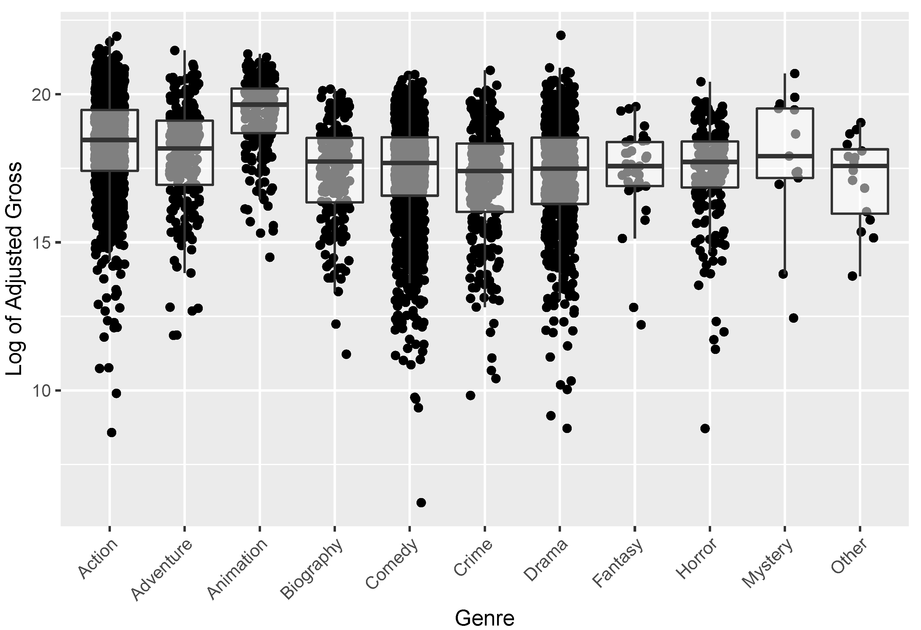
  • genre: levels of action, adventure, biography, comedy, crime, drama, fantasy, horror, mystery and other
  • season: levels of fall, winter, spring, and summer
  • adjustedBudget: measured in United States dollars
  • adjustedGross: measured in United States dollars
  • year: ranges from 1980 to 2020.
Table 1 shows summary statistics for the rating and season variables. From the table, we can see that for our dataset, the most frequent rating was R with 2036 observations followed by PG-13 with 1448. Additionally, regardless of whether we look at the mean or the median, G movies grossed the most followed by PG, then PG-13, then R, and then Other at the bottom. From Table 1, we can see that there was a fairly even distribution of movies throughout the four seasons. We can see that each season had around 1000–1100 observations. Looking at the median adjusted gross, we can see that summer movies appeared to make the most money followed by winter movies, then spring movies, and then fall movies in last place.
Figure 1 shows side-by-side boxplots for each genre against the log of adjustedGross. The log of adjustedGross was taken for Figure 1 in order to more effectively demonstrate the differences in the genres in terms of adjustedGross. From Figure 1, we can see that there is not much of a difference in the boxplots in terms of interquartile range. However, we can see that the genre of animation has a much higher median than the other genres. Therefore, there is visual evidence to suggest that Animation movies gross more than the other genres in terms of the measure of center. Figure 2 demonstrates how the median adjusted gross of movies has changed over the years. The median was used instead of the mean due to the adjustedGross variable being heavily skewed to the right. From Figure 2, we can see that there is visual evidence to suggest that as the years have gone by, the median adjusted gross of movies has increased. We note that the big spike in median adjusted gross in the year 2020 is most likely a byproduct of the fact that the number of 2020 movies in the dataset was low (five movies).

3. Statistical Methods

3.1. Multiple Linear Regression

First, we considered a multiple linear regression model. The regression model was built such that adjustedGross was the response variable and rating, year, genre, season, and adjustedBudget were the explanatory variables. When we perform multiple linear regression, there are four assumptions that should be met. The assumptions are as follows: residuals are evenly distributed around zero, homoscedasticity (residuals have constant variance), residuals are normally distributed, and observations are independent. If these assumptions are violated, then one must be careful about interpreting model effects, as those interpretations may be inaccurate [20]. We can examine model diagnostic plots to check whether our linear regression model meets these assumptions.
Figure 3 shows that there appears to be a trend in the residuals, suggesting that the residuals are not evenly distributed around zero. Additionally, we can see that there appears to be non-constant variance in the residuals. The variation in the residuals appears to become larger as fitted values increases. This is a signal that our residuals exhibit the property of heteroscedasticity (non-constant variance) and thus violate the assumption that the residuals are homoscedastic. The normal quantile-quantile plot on the right in Figure 3 is used to check whether the residuals are normally distributed. From the normal quantile-quantile plot, we can see that residuals deviate from the straight line at both the lower and upper quantiles. This deviation from the straight line signifies that the residuals are not normally distributed and are in violation of the normal distribution assumption. Thus, we can see that the linear regression model of adjustedGross as the response and adjustedBudget, year, season, genre, and rating as the independent variables violates three of the four linear regression model assumptions. The violation of the model assumptions means that the standard errors for the model coefficients and the associated confidence intervals/p-values may be inaccurate.
To rectify these model violations, we tried to transform the model’s variables (i.e., adjustedBudget, year, and adjustedGross). In order to check what kind of transformation we should apply to those variables, we can examine the distributions of each one. Figure 4 shows the distributions of the year, adjustedBudget, and adjustedGross variables. From Figure 4, we can see that both the adjustedBudget and adjustedGross variables appear to be heavily skewed to the right. This means that some movies in the dataset had either an unusually high adjustedBudget, an unusually high adjustedGross, or both. We can also see that the year variable appears to be roughly normally distributed. The severe skewness of the adjustedBudget and adjustedGross variables are most likely causing problems with the multiple linear regression model and contributing to the violation of the model assumptions. As such, we can attempt to take the log of the adjustedBudget and adjustedGross variables in an attempt to normalize their distributions.
Figure 5 shows the distributions of the year and logged versions of the adjustedBudget and adjustedGross variables. From Figure 5 we can see that taking the log of the adjustedBudget and adjustedGross variables has resulted in the two variables being skewed to the left instead of the right. However, the left skewness does not appear to be as severe as the right skewness that can be seen in Figure 4. Thus, we can see that although taking the log of adjustedBudget and adjustedGross has resulted in them becoming skewed left, they are more normally distributed than they were before. Since the logged versions of adjustedBudget and adjustedGross appear to be more normally distributed than their non-logged counterparts, we can build a new multiple linear regression model with the logged versions of both the adjustedBudget and adjustedGross variables to see if this new model performs better in regards to the model assumptions.
The logged version of multiple linear regression is given below:
l o g ( a d j u s t e d G r o s s ) = y e a r + s e a s o n + r a t i n g + g e n r e + l o g ( a d j u s t e d B u d g e t ) .
The untransformed linear regression model had an AIC score of 176,322 whereas the AIC score for the transformed model had an AIC score of 14,781. This dramatic drop in AIC score suggests that the model with the logs of adjustedBudget and adjustedGross is a better fitting model than the untransformed multiple linear regression model. However, even though the AIC score suggests that the transformed model is a better fit for the data than the untransformed model, that does not mean it is appropriate to use, and we still need to check model assumptions using diagnostic plots.
The diagnostic plots for the transformed model can be found in Figure 6. From the Residuals vs. Fitted Values plot on the left, we can see that we still have the same problems that we had with the untransformed multiple linear regression model. There still appears to be a trend in the residuals, indicating that the residuals are not evenly spread around zero. The issue of heteroscedasticity also remains a problem, as the variation in the residuals appears to be decreasing as Fitted Values increase. The normal quantile-quantile plot on the right in Figure 6 still shows evidence of the residuals being non-normally distributed. The residuals appear to be normally distributed at the middle and upper quantiles but deviate from the straight line at the lower quantiles. Therefore, despite the fact that the transformed model is a better fitting model than the untransformed one, the transformed model still violates three of the four linear regression model assumptions, and thus the p-values, confidence intervals, and standard errors for the model coefficients may be inaccurate. Thus, we need to consider a different approach to ensure that interpretations will be accurate. We apply our movie data to a copula-based regression model which does not need independent, linearity, normality, and constant variance assumptions.

3.2. Gaussian Copula Marginal Regression and Vine Copula

A copula is a multivariate distribution function defined on the unit [ 0 , 1 ] n , with uniformly distributed marginals. Ref. [14] shows that any bivariate distribution function, F ( y 1 , y 2 ) , can be represented as a function of its marginal distribution of Y 1 and Y 2 , F ( y 1 ) and F ( y 2 ) , by using a two-dimensional copula C ( · , · ) . More specifically, the copula may be written as
F ( y 1 , y 2 ) = C ( F ( y 1 ) , F ( y 2 ) ) = C ( u , v ) ,
where u and v are the continuous empirical marginal distribution function F ( y 1 ) and F ( y 2 ) , respectively. Note that u and v have uniform distribution U ( 0 , 1 ) .
Therefore, the copula function represents how the function, F ( y 1 , y 2 ) , is coupled with its marginal distribution functions, F ( y 1 ) and F ( y 2 ) . It also describes the dependence mechanism between two random variables by eliminating the influence of the marginals or any monotone transformation of the marginals. Our study employs the Gaussian copula regression method to measure the relationship between two variables. Let F ( · | x i ) be the marginal cumulative distribution for x i , then the joint cumulative distribution function in the Gaussian copula regression can be expressed
Pr ( Y 1 y 1 ,   ,   Y n y n ) = Φ n ϵ 1 ,   ,   ϵ n ; P ,
where ϵ i = Φ 1 F ( y i | x i ) . For the correlation matrix of the Gaussian copula P, the standard normal univariate and multivariate cumulative distribution functions are Φ ( · ) and Φ n ( · ; P ) . See [15] for more details. In particular, ref. [15] introduces an equivalent formulation of the Gaussian copula model as follows:
Y i = h ( x i , ϵ i ) ,
where ϵ i indicates a stochastic error that follows a multivariate standard normal distribution with correlation matrix P. Note that h ( x i , ϵ i ) = F 1 Φ ( ϵ i ) | x i is assumed in the Gaussian copula regression model.
In the bivariate case, Gaussian copula, t copula, and Archimedean copula families are available in practice and have been extensively studied in literature [12,13]. However, the selection of an appropriate copula in higher dimensional problem is not easy because standard multivariate copulas have limitations such that one or two parameters explain multivariate dependence structure. In order to overcome these problems, vine copulas are proposed by [21] and explained in more detail by [22,23,24]. Vine copulas are a graphical model that represent a d-dimensional multivariate density in a hierarchical manner. The canonical (C-) vines and the D-vines [25] have been widely used in [26,27,28,29,30,31,32,33]. The C-vines need to designate the relationship order between one specific variable and the remaining variables, but D-vines are free to select which pairs for modeling the dependence. The d-dimensional D-vine density, given by [24], is
f ( y ; ϕ ) = k = 1 d f k y k × i = 1 d 1 j = 1 d i c j , j + i ( j + 1 ) : ( j + i 1 ) F y j y j + 1 ,   ,   y j + i 1 , F y j + i y j + 1 ,   ,   y j + i 1 ; β j , j + i ( j + 1 ) : ( j + i 1 ) ,
where f k x k are the marginal densities, c j , j + i ( j + 1 ) : ( j + i 1 ) are the bivariate copula densities with parameter(s) β j , j + i ( j + 1 ) : ( j + i 1 ) and ϕ is the set of all parameters in the D-vine density.

4. Copula Data Analysis

To overcome the difficulties of multiple linear regression in the previous section, we apply the movie data to the GCMR and vine copula regression models. First, we apply a GCMR model to the data by using the gcmr R package. For our data analysis, GCMR models enable one to specify the correlation matrix of the errors. For this study, correlation matrices of autoregressive moving average (ARMA)(0, 0), ARMA(0, 1), ARMA(1, 0), and ARMA(1, 1) were considered. To select the best GCMR model with the correlation matrix, four different GCMR models were compared with Akaike information criterion (AIC). The GCMR models were built such that adjustedGross was the response and the explanatory variables were adjustedBudget, rating, year, season, and genre. Table 2 has the AIC scores of the four GCMR models. From Table 2, we can see that the second GCMR model with a correlation matrix of ARMA(1, 1) (modGCMR2) has the lowest AIC score out of the four models. This means that there is evidence to suggest that the GCMR model with a correlation matrix of ARMA(1, 1) is the best fitting model. Therefore, we will use the GCMR model with a correlation matrix of ARMA(1, 1) for our analysis and interpretations.
Table 3 shows that as the years have gone by movies have grossed more money, and this idea is reinforced by the GCMR model’s estimated coefficient for year ( β ^ = 932,800, p-value = 0.000). An estimated coefficient of 932,800 and a p-value below the 0.05 cutoff value means that there is statistical evidence that as the year increases by one year, there is a USD 932,800 increase in adjustedGross, after adjusting for season, adjustedBudget, rating, and genre.
Examining the GCMR model rating coefficients relative to the reference level (Rating G) in Table 3 reveals that Rating G movies gross more than any other genre after adjusting for year, adjustedBudget, genre, and season. In terms of our GCMR model, the reference level was the Action genre. Thus, the model coefficients for the GCMR model are relative to the action genre. Examining the GCMR model revealed that there is evidence to suggest that Action movies gross more than the biography ( β ^ = 7,783,000, p = 0.000 ), comedy ( β ^ = 63,970, p = 0.000 ), crime ( β ^ = 3 , 041 , 000 , p = 0.000 ) and other ( β ^ = 37,120,000, p = 0.000 ) genres, after adjusting for season, adjustedBudget, rating, and year. There was also evidence to suggest that action movies gross less than adventure ( β ^ = 6,948,000, p = 0.000 ), animation ( β ^ = 83,410,000, p = 0.000 ), drama ( β ^ = 10,320,000, p = 0.000 ), fantasy ( β ^ = 2 , 675 , 000 , p = 0.000 ), horror ( β ^ = 42,060,000, p = 0.000 ), and mystery ( β ^ = 70,180,000, p = 0.000 ) genres. The reference level for the GCMR model was fall, so all of the model coefficients are relative to fall. Looking at the model coefficients: spring: ( β ^ = 21,200,000, p = 0.000 ), winter: ( β ^ = 13,280,000, p = 0.000 ), summer: ( β ^ = 29,630,000, p = 0.000 ). We can see that there is statistical evidence to suggest that fall movies gross 21,200,000 dollars less than spring movies, 13,280,000 dollars less than winter movies, and 29,630,000 dollars less than summer movies after adjusting for year, rating, genre, and adjustedBudget.
The increasing effect that adjustedBudget has on adjustedGross is again reinforced by our GCMR model, as the model coefficient for the adjustedBudget variable was ( β ^ = 2.727 , p = 0.000 ). The p-value for the model coefficient is far below the 0.05 significance cutoff value. Thus, there is evidence to suggest that a one dollar increase in adjustedBudget is associated with a USD 2.727 increase in adjustedGross, after adjusting for season, year, rating, and genre. The sigma in Table 3 is a dispersion parameter for error in the GCMR model. It is statistically significant to adjust the non-constant variance of the errors. AR(1) and MA(1) in Table 3 are statistically significant to fit the correlation matrix of the errors. Figure 7 shows the residual plot, ACF plot, and partial ACF plot. ACF is an autocorrelation function that gives us values of autocorrelation of any series with its lagged values. PACF is a partial autocorrelation function and finds a correlation of the residuals with the next lag value. In Figure 7, the residual plot shows a flat pattern, and the ACF and partial ACF plots show a stationary time series pattern.
Figure 8 is a graph of the effect of adjustedBudget on adjustedGross from a D-vine copula regression model constructed using the vinereg R package (see [34] for understanding C- and D-Vine Copulas). The D-vine copula model also had the same response (adjustedGross) variable and explanatory variables (year, season, rating, genre, adjustedBudget) as the GCMR model. The D-vine copula model was constructed as the gcmr R package does not have efficient methods to graph model effects. We considered D-vine-based quantile regression with all copula parametric and nonparametric families [35]. We found statistically significant adjustedBudget explanatory variable to response adjustedGross variable across the quantiles, which are specified in the graph legend in Figure 8. From the Figure 8, we can see that there is a relationship between adjustedBudget and adjustedGross. We can see that for each quantile, it appears that adjustedBudget is associated with an increase in adjustedGross, with the positive effect that adjustedBudget has on adjustedGross being stronger in the higher quantiles.

5. Conclusions

We analyzed movie data that were adjusted for inflation using a CPI table, and the data were applied to the GCMR and vine copula regression models due to violations of multiple linear regression model assumptions. From our data analysis by the GCMR, we found that year, budget, genre, rating, and season were all statistically significant predictors of gross. Specifically, this study found that there was evidence to suggest that year was associated with an increase in movie gross, with a one year increase being associated with a USD 932,800 increase in movie gross, after adjusting for the other predictors. We also found that action movies were also found to gross more money than the biography, comedy, crime, and other movie genres, but gross less money than adventure, animation, drama, fantasy, horror, and mystery movies after adjusting for season, year, budget, and rating. Our finding suggested that Rating G movies were found to gross more money than all other ratings, after adjusting for season, year, budget, and genre. Fall movies were found to bring in the least amount of gross compared to the other three seasons, after adjusting for year, budget, genre, and rating. Finally, a one dollar increase in budget was associated with a 2.727 dollar increase in movie gross, after adjusting for season, rating, genre, and year. Finally, future studies will consider investigating polarization in movie critic and audience review scores with the GCMR model. Finally, future studies may consider investigating the polarization of movie critic and audience review scores with the GCMR model. In our future study, we will consider the prediction of international movie gross based on the GCMR and vine copula models and try to visualize the time course pattern clustering by functional principal component analysis.

Author Contributions

Conceptualization, J.E.; methodology, J.-M.K.; software, J.E.; validation, J.E. and J.-M.K.; formal analysis, J.E.; investigation, J.E. and J.-M.K.; resources, J.E.; data curation, J.E.; writing—original draft preparation, J.E. and J.-M.K.; writing—review and editing, J.E. and J.-M.K.; visualization, J.E.; supervision, J.-M.K.; project administration, J.-M.K. All authors have read and agreed to the published version of the manuscript.

Funding

This research received no external funding.

Institutional Review Board Statement

Not applicable.

Informed Consent Statement

Not applicable.

Data Availability Statement

Not applicable.

Acknowledgments

The authors would like to thank the editor and the two anonymous respected referees for their suggestions, which have greatly improved the paper.

Conflicts of Interest

The authors declare no conflict of interest.

References

  1. Childress, E.; Staff, R.T. The 50 Highest-Grossing Movies of All Time: Your Top Box Office Earners Ever Worldwide. Rotten Tomatoes. 24 February 2022. Available online: https://editorial.rottentomatoes.com/article/highest-grossing-movies-all-time/ (accessed on 3 March 2022).
  2. McClintock, P. Global Box Office Revenue Hits Record $41B in 2018, Fueled by Diverse U.S. Audiences. The Hollywood Reporter. 21 March 2019. Available online: https://www.hollywoodreporter.com/news/general-news/global-box-office-revenue-hits-record-41b-2018-fueled-by-diverse-us-audiences-1196010/ (accessed on 3 March 2022).
  3. Chang, B.-H.; Ki, E.-J. Devising a practical model for predicting theatrical movie success: Focusing on the experience good property. J. Media Econ. 2005, 18, 247–269. [Google Scholar] [CrossRef]
  4. Lash, M.T.; Zhao, K. Early Predictions of Movie Success: The Who, What, and When of Profitability. J. Manag. Inf. Syst. 2016, 33, 874–903. [Google Scholar] [CrossRef] [Green Version]
  5. Ho, J.Y.C.; Krider, R.E.; Chang, J. Mere newness: Decline of movie preference over time. Can. J. Adm. Sci. 2017, 34, 33–46. [Google Scholar] [CrossRef]
  6. Du, J.; Xu, H.; Huang, X. Box office prediction based on microblog. Expert Syst. Appl. 2014, 41, 1680–1689. [Google Scholar] [CrossRef]
  7. Lee, K.; Park, J.; Kim, I.; Choi, Y. Predicting movie success with machine learning techniques: Ways to improve accuracy. Inf. Syst. Front. 2018, 20, 577–588. [Google Scholar] [CrossRef] [Green Version]
  8. Liu, Y.; Xie, T. Machine learning versus econometrics: Prediction of box office. Appl. Econ. Lett. 2019, 26, 124–130. [Google Scholar] [CrossRef]
  9. Xiao, X.; Cheng, Y.; Kim, J.-M. Movie Title Keywords: A Text Mining and Exploratory Factor Analysis of Popular Movies in the United States and China. J. Risk Financ. 2021, 14, 68. [Google Scholar] [CrossRef]
  10. Kim, J.-M.; Xia, L.; Kim, I.-S.; Lee, S.-J.; Lee, K.-H. Finding Nemo: Predicting Movie Performances by Machine Learning Methods. J. Risk Financ. Manag. 2020, 13, 93. [Google Scholar] [CrossRef]
  11. Kim, J.-M.; Xiao, X.; Kim, I.-S. Hollywood Movie Analysis by Social Network Analysis and Text Mining. Int. Electron. Commer. Stud. 2020, 11, 75–92. [Google Scholar] [CrossRef]
  12. Joe, H. Multivariate Models and Multivariate Dependence Concepts; CRC Press: Boca Raton, FL, USA, 1997. [Google Scholar]
  13. Nelsen, R.B. An Introduction to Copulas, 2nd ed.; Springer Science & Business Media: Berlin/Heidelberg, Germany, 2013. [Google Scholar]
  14. Sklar, A. Fonctions de Repartition á n Dimensions et Leurs Marges; Publications de l’Institut de Statistique de l’Université de Paris: Paris, France, 1959; Volume 8, pp. 229–231. [Google Scholar]
  15. Masarotto, G.; Varin, C. Gaussian copula marginal regression. Electron. J. Stat. 2020, 6, 1517–1549. [Google Scholar] [CrossRef]
  16. Cherubini, U.; Luciano, E.; Vecchiato, W. Copula Methods in Finance; John Wiley: Chichester, UK, 2004. [Google Scholar]
  17. Kim, J.-M. A Review of Copula Methods for Measuring Uncertainty in Finance and Economics. Quant. Bio-Sci. 2020, 39, 81–90. [Google Scholar]
  18. Kim, J.M.; Jung, H. Relationship between Oil Price and Exchange Rate by FDA and Copula. Appl. Econ. 2018, 50, 2486–2499. [Google Scholar] [CrossRef]
  19. Kim, J.-M.; Kim, D.H.; Jung, H. Modeling Non-normal Corporate Bond Yield Spreads by Copula. N. Am. Econ. Financ. 2020, 53, 101210. [Google Scholar] [CrossRef]
  20. McCullagh, P.; Nelder, J.A. Generalized Linear Models; Chapman and Hall: New York, NY, USA, 1989. [Google Scholar]
  21. Joe, H. Families of m-variate distributions with given margins and m(m − 1)/2 bivariate dependence parameters. In Distributions with Fixed Marginals and Related Topics; Rüschendorf, L., Schweizer, B., Taylor, M.D., Eds.; Institute of Mathematical Statistics: Washington, DC, USA, 1996; pp. 120–141. [Google Scholar]
  22. Bedford, T.; Cooke, R.M. Vines—A new graphical model for dependent random variables. Ann. Stat. 2002, 30, 1031–1068. [Google Scholar] [CrossRef]
  23. Aas, K.; Berg, D. Models for construction of multivariate dependence: A comparison study. Eur. Financ. 2009, 15, 639–659. [Google Scholar] [CrossRef]
  24. Aas, K.; Czado, C.; Frigessi, A.; Bakken, H. Pair-copula constructions of multiple dependence. Insur. Math. Econ. 2009, 44, 182–198. [Google Scholar] [CrossRef] [Green Version]
  25. Kurowicka, D.; Cooke, R.M. Distribution—Free continuous bayesian belief nets. In Proceedings of the Fourth International Conference on Mathematical Methods in Reliability Methodology and Practice, Santa Fe, NM, USA, 21–25 June 2004. [Google Scholar]
  26. Bauer, A.; Czado, C.; Klein, T. Pair-copula constructions for non-Gaussian DAG models. Can. J. Stat. 2012, 40, 86–109. [Google Scholar] [CrossRef] [Green Version]
  27. Brechmann, E.; Czado, C.; Aas, K. Truncated and simplified regular vines in high dimensions with application to financial data. Can. J. Stat. 2012, 40, 68–85. [Google Scholar] [CrossRef]
  28. Hobæk Haff, I.; Aas, K.; Frigessi, A. On the simplified pair-copula construction—Simply useful or too simplistic? J. Multivar. Anal. 2010, 101, 1296–1310. [Google Scholar] [CrossRef] [Green Version]
  29. Panagiotelis, A.; Czado, C.; Joe, H. Pair Copula Constructions for Multivariate Discrete Data. J. Am. Stat. Assoc. 2012, 107, 1063–1072. [Google Scholar] [CrossRef]
  30. Smith, M.; Min, A.; Almeida, C.; Czado, C. Modelling longitudinal data using a pair-copula decomposition of serial dependence. J. Am. Stat. 2010, 105, 1467–1479. [Google Scholar] [CrossRef]
  31. Kim, D.; Kim, J.-M.; Liao, S.-M.; Jung, Y. Mixture of D-vine Copula Approach for Modeling Dependence. Comput. Data Anal. 2013, 64, 1–19. [Google Scholar] [CrossRef]
  32. Pourkhanali, A.; Kim, J.-M.; Tafakori, L.; Fard, F.A. Measuring Systemic Risk Using VineCopula. Econ. Model. 2016, 53, 63–74. [Google Scholar] [CrossRef]
  33. Jang, H.; Kim, J.-M.; Noh, H. Vine Copula Granger Causality in Mean. Econ. Model. 2022, 109, 105798. [Google Scholar] [CrossRef]
  34. Brechmann, E.C.; Schepsmeier, U. Modeling Dependence with C- and D-Vine Copulas: The R Package CDVine. J. Stat. Softw. 2013, 52, 1–27. [Google Scholar] [CrossRef] [Green Version]
  35. Kraus, D.; Czado, C. D-vine copula based quantile regression. Comput. Stat. Data Anal. 2017, 110, 1–18. [Google Scholar] [CrossRef] [Green Version]
Figure 1. Side-by-side boxplots of genre against log of adjusted gross.
Forecasting 04 00037 g001
Figure 2. Graph of median adjusted gross per year.
Forecasting 04 00037 g002
Figure 3. Checking multiple linear regression model assumptions.
Forecasting 04 00037 g003
Figure 4. Checking distributions of numerical variables in our multiple linear regression model.
Forecasting 04 00037 g004
Figure 5. Checking distributions of numerical variables. This time we have taken the log of adjustedBudget and adjustedGross.
Forecasting 04 00037 g005
Figure 6. Checking multiple linear regression model assumptions of transformed model.
Forecasting 04 00037 g006
Figure 7. Plots of GCMR model with ARMA(1, 1) error correlation matrix.
Forecasting 04 00037 g007
Figure 8. Dependence between adjustedBudget and adjustedGross.
Forecasting 04 00037 g008
Table 1. Summary statistics for the rating and season variables.
VariableMean Adjusted GrossMedian Adjusted GrossCount
G332,980,911217,551,76480
Rating PG201,944,37292,265,952730
Rating PG-13196,379,10690,102,6071448
Rating R86,180,46437,829,0742036
Rating Other4,734,2531,935,22028
Summer183,515,78286,822,2411162
Winter136,243,16868,325,0931017
Spring154,837,91252,443,9681018
Fall110,738,80843,177,2731125
Table 2. AIC scores for the various GCMR models. modGCMR has a correlation matrix of (0, 0), modGCMR2 has a correlation matrix of (1, 1), modGCMR3 has a correlation matrix of (1, 0), and modGCMR4 has a correlation matrix of (0, 1).
ModelAIC
modGCMR176,322.1
modGCMR2175,865.9
modGCMR3176,161.2
modGCMR4176,211.5
Table 3. modGCMR2 coefficients and p-vlaue relative to the reference level (Rating G, action movie, fall.
EstimateStd. Errorp-Value
(Intercept)−1,878,000,0000.000000000050.000
year932,8000.000000107000.000
ratingOther−14,460,0000.000000000010.000
ratingPG−8,075,0000.000000000070.000
ratingPG-13−16,860,0000.000000000100.000
ratingR−27,640,0000.000000000130.000
genreAdventure6,948,0000.000000000010.000
genreAnimation83,410,0000.000000000060.000
genreBiography−7,783,0000.000000000010.000
genreComedy−63,9700.000000000060.000
genreCrime−3,041,0000.000000000020.000
genreDrama10,320,0000.000000000030.000
genreFantasy2,675,0000.000000000000.000
genreHorror42,060,0000.000000000030.000
genreMystery70,180,0000.000000000000.000
genreOther−37,120,0000.000000000000.000
seasonSpring21,200,0000.000000000030.000
seasonSummer29,630,0000.000000000040.000
seasonWinter13,280,0000.000000000000.000
adjustedBudget30.047970000000.000
sigma174,000,0000.000000000250.000
AR(1)0.9570430.0071220.000
MA(1)−0.799550.0168510.000
Publisher’s Note: MDPI stays neutral with regard to jurisdictional claims in published maps and institutional affiliations.

