Abstract
Deep neural networks (DNNs) are prominent in predictive analytics for accurately forecasting target variables. However, inherent uncertainties necessitate constructing prediction intervals for reliability. The existing literature often lacks practical methodologies for creating predictive intervals, especially for time series with trends and seasonal patterns. This paper explicitly details a practical approach integrating dual-output Monte Carlo Dropout (MCDO) with DNNs to approximate predictive means and variances within a Bayesian framework, enabling forecast interval construction. The dual-output architecture employs a custom loss function, combining mean squared error with Softplus-derived predictive variance, ensuring non-negative variance values. Hyperparameter optimization is performed through a grid search exploring activation functions, dropout rates, epochs, and batch sizes. Empirical distributions of predictive means and variances from the MCDO demonstrate the results of the dual-output MCDO DNNs. The proposed method achieves a significant improvement in forecast accuracy, with an RMSE reduction of about 10% compared to the seasonal autoregressive integrated moving average model. Additionally, the method provides more reliable forecast intervals, as evidenced by a higher coverage proportion and narrower interval widths. A case study on Thailand’s durian export data showcases the method’s utility and applicability to other datasets with trends and/or seasonal components.
1. Introduction
In the field of predictive analytics, there is a growing need for models that can accurately forecast outcomes while also providing measures of the associated uncertainties. This requirement is particularly critical in time-series forecasting, where decisions often need to be made under uncertain circumstances. Accurate time-series forecasts are essential across various domains, including finance, healthcare, and supply chain management, as they facilitate strategic planning and enhance decision-making processes. However, traditional forecasting methods such as the autoregressive integrated moving average (ARIMA) and seasonal autoregressive integrated moving average (SARIMA), while effective in handling linear patterns and seasonal effects, often fall short in capturing the complex non-linear relationships present in real-world data. Moreover, these methods typically do not provide inherent measures of uncertainty, which are crucial for risk management and informed decision-making.
To address these limitations, dropout techniques have been introduced in neural networks as a practical method to approximate Bayesian inference. Gal and Ghahramani [1] proposed using dropouts in neural networks to measure model uncertainty, offering a theoretical framework for this approach. Building on this, Kendall and Gal [2] expanded the use of Monte Carlo Dropout (MCDO) to differentiate between aleatoric and epistemic uncertainties in deep learning models. Srivastava et al. [3] demonstrated the effectiveness of dropout as a regularization technique in improving neural network performance across tasks such as vision, speech recognition, and document classification. Zhang et al. [4] utilized Bayesian networks for predicting short-term traffic flow, highlighting the importance of uncertainty estimation in practical applications. Pearce et al. [5] merged Bayesian neural networks (BNNs) with deep ensemble methods, showcasing enhanced uncertainty estimation for predictions, particularly in time-series forecasting. Fortunato et al. [6] further demonstrated that a minor modification of the truncated backpropagation through time can significantly enhance regularization and uncertainty estimates with minimal computational cost and an 80% reduction in the number of parameters.
Blundell et al. [7] introduced a variational inference approach to quantify uncertainty in neural network weights, indirectly supporting the methodology behind using dropout for uncertainty estimation in time-series forecasting. This approach aligns with the dual-output MCDO methodology proposed in our study, where we aim to improve interval forecasting for time-series data.
Recent studies have further explored and improved uncertainty estimation in neural networks. Srisuradetchai et al. [8] introduced the artificial neural network with best subset selection (ANNBS) to improve prediction accuracy by selecting an optimum subset of variables using a Monte Carlo algorithm, significantly enhancing predictive performance by reducing root mean square errors (RMSEs) for both the training and test data. Fan et al. [9] presented a deep learning framework with temporal mechanisms to capture latent patterns important for precise future predictions, generating forecasts for various timeframes and quantiles simultaneously. Lemay et al. [10] evaluated the consistency of artificial intelligence models in clinical processes, highlighting how MCDO predictions improve model repeatability and classification accuracy. Alahmari et al. [11] examined the reliability of deep learning models for segmentation and classification tasks using U-Net and LeNet-5 frameworks, emphasizing the robustness of MCDO in these applications.
Hinton et al. [12] suggested a dropout technique to reduce overfitting in large feed-forward neural networks trained on small datasets, improving generalization by preventing feature detectors from co-adapting. Camarasa et al. [13] demonstrated the effectiveness of MCDO for quantifying uncertainty in multi-class segmentation tasks, enhancing the reliability of uncertainty maps in predicting misclassifications. Leibig et al. [14] showed that dropout-based Bayesian uncertainty measures effectively capture decision-making uncertainty in disease detection with deep neural networks, surpassing traditional methods.
García González et al. [15] examined the role of time-series data augmentation and dropout in enhancing deep learning models for fall detection, while Maleki Sadr et al. [16] developed an anomaly detection method for satellite telemetry using an MCDO-based approximation of BNNs. Atencia et al. [17] combined echo state networks (ESNs) with MCDO to quantify uncertainty in time-series prediction without increasing computational expenses. Sheng et al. [18] created a bootstrapping reservoir computing network ensemble (BRCNE) to generate accurate prediction intervals in noisy non-linear time-series forecasting. Khosravi et al. [19] proposed creating prediction intervals for travel time forecasts using delta and Bayesian methods, evaluating the accuracy and reliability of these predictions.
Despite advances, practical methods for constructing prediction intervals for time-series data with trends and seasonal patterns are still lacking. Point predictions often overlook uncertainty, necessitating new models that incorporate comprehensive uncertainty estimation. This study introduces a prediction interval generation method combining dual-output MCDO with deep neural networks (DNNs). Using a Bayesian framework, it efficiently estimates predictive means and variances. This approach is validated with Thailand’s durian export data, which has significant seasonal variations and trends.
The proposed methodology addresses a critical gap in forecasting techniques as follows:
- Comprehensive uncertainty estimation: provides both aleatoric and epistemic uncertainties, offering a complete uncertainty profile;
- Improved forecast accuracy: achieves a lower RMSE compared to traditional models like SARIMA;
- Practical application: demonstrated effectiveness on real-world data with significant seasonal variations and trends;
- Enhanced model regularization: utilizes dropout techniques to prevent overfitting, ensuring robust performance;
- Flexible architecture: capable of handling complex, non-linear relationships in time-series data.
2. Related Theories
2.1. Aleatoric and Epistemic Uncertainties
2.1.1. Aleatoric Uncertainty
Aleatoric uncertainty is captured directly through the predictive variance in a dual-output configuration. It is also known as data uncertainty and cannot be reduced even if more data are collected. In the context of neural networks, aleatoric uncertainty is captured directly by the network through the predictive variance output by one of the network heads.
Let be the actual target value, be the predicted mean output by the first head of the network, and be the predicted variance output by the second head of the network, representing the aleatoric uncertainty. The network is trained to minimize a loss function that incorporates both the prediction error and the uncertainty estimation. The mean squared error (MSE) modified to include the aleatoric uncertainty can be expressed as follows:
where the first term weights the squared prediction error by the inverse of the predicted variance, emphasizing predictions with lower uncertainty; the second term acts as a regularizer to prevent the network from predicting infinite variance for reducing the prediction error term [20].
2.1.2. Epistemic Uncertainty
This type of uncertainty arises from the model itself due to limited data or knowledge about the model parameters. It is also known as model uncertainty and can be reduced by gathering more data. Epistemic uncertainty is estimated through the variance in predictions across multiple stochastic forward passes with dropout enabled, simulating a Bayesian posterior distribution. Let T be the number of stochastic forward passes, be the prediction for the i-th instance in the -th forward pass. The epistemic uncertainty can be quantified as the variance of the following predictions:
where is the mean prediction across all stochastic forward passes for the i-th instance. Combining both uncertainties, the total predictive uncertainty can be seen as the sum of aleatoric and epistemic uncertainties [21].
2.2. Deep Neural Networks
A deep neural network (DNN) is a type of machine learning model that belongs to a broader category of structures designed to represent sophisticated functions. These models are composed of multiple layers of units, or neurons, where each layer performs a transformation of its inputs, typically followed by a non-linear activation function. In mathematical terms, a DNN can be defined as a composition of functions, each representing a layer in the network.
For a DNN with L layers, the function f representing the network is composed of L functions , each corresponding to a layer. The output of each layer function is the input to the next layer. This can be expressed as follows:
where is the input vector, Θ denotes the set of all parameters in the network, and represents the parameters for the -th layer. Each layer function is typically a linear transformation followed by a non-linear activation:
where is a weight matrix, is a bias vector, and is the activation function for the -th layer [22,23].
2.3. Activation Functions
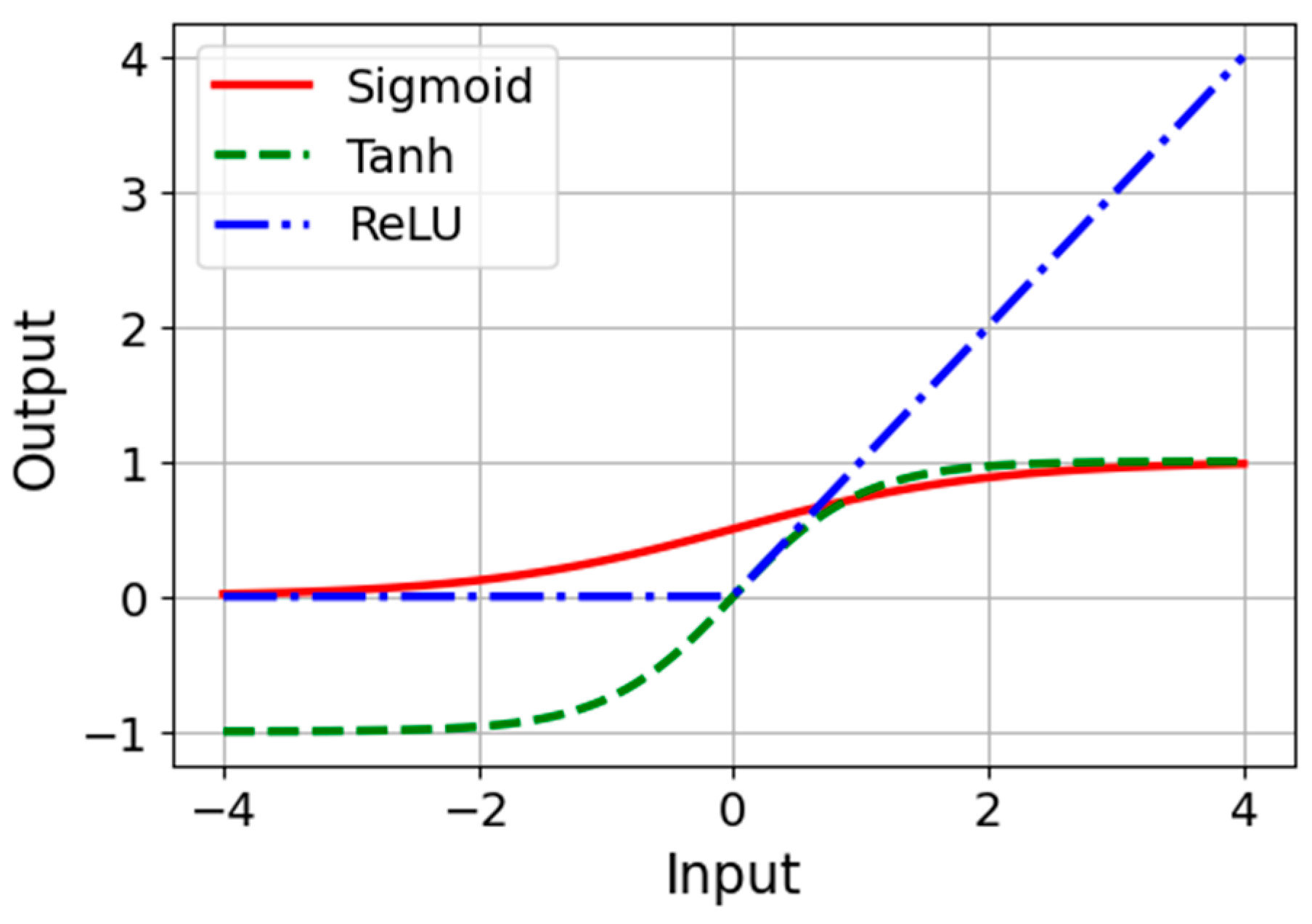
A common choice for the activation function includes non-linear functions like the Rectified Linear Unit (ReLU), Sigmoid, or hyperbolic tangent (Tanh). The choice of activation function and the architecture of the network determine the function class that the DNN can approximate.
Figure 1 illustrates Sigmoid, Tanh, and ReLU. Each function maps the input signal to an output signal and serves as a gate, determining whether and how signals should progress through the network. Details on each activation function are as follows [24]:
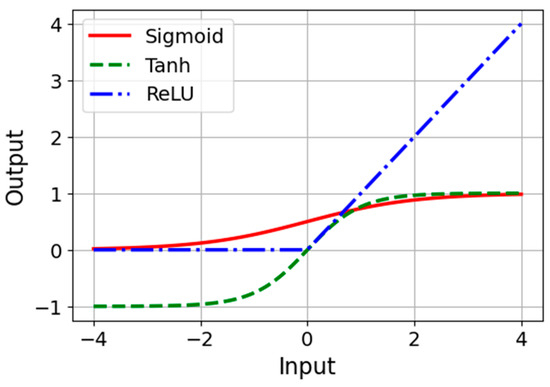
Figure 1.
Activation functions.
- The Sigmoid function is defined as σ(x) = 1/(1 + exp(−x)), and it outputs values between 0 and 1. It is a smooth, S-shaped curve that has been widely used historically, especially for binary classification problems;
- The Tanh function or hyperbolic tangent function, tanh(x), rescales the sigmoid to output values between −1 and 1. It is zero-centered, making it preferred in certain scenarios as it can help with improving the convergence during the training phase;
- The ReLU function, defined as ReLu(x) = max(0,x), activates a neuron only if the input is above zero, providing a piecewise linear output that is computationally efficient and enables the model to leverage sparsity for better performance and faster training.
In the dual-output architecture of the neural network, the Softplus activation function is employed for the variance output layer. This choice is strategic; Softplus, defined mathematically as f(x) = log(1 + exp(x)), is smooth and differentiable, making it well-suited for predicting positive continuous variables, such as variance, which must be non-negative. Its application ensures that the network predicts a variance that is not only always positive but also has a gradient that allows for effective backpropagation and learning of uncertainty in the data [25].
2.4. Regularization
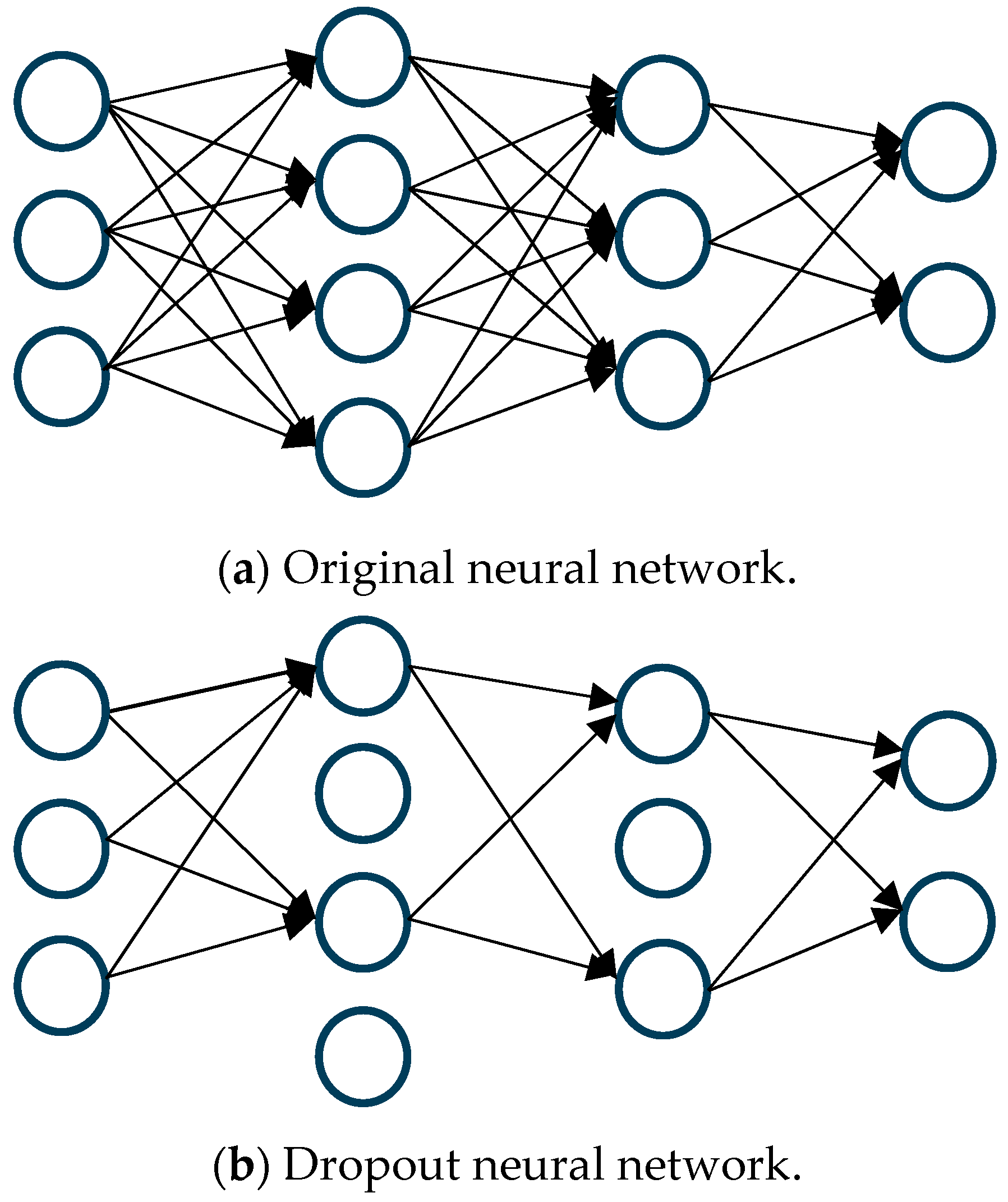
One widely recognized technique for regularization is known as dropout, a process where connections within the network are probabilistically excluded in each iteration of training [3]. This method is visually represented in Figure 2, where a standard neural network, (a) before and (b) after the application of dropout, is depicted.
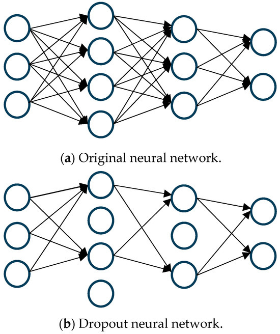
Figure 2.
Neural network (a) before and (b) after applying dropout. Arrows represent connections; missing arrows in (b) indicate dropout.
In this process, if wij is the weight of the connection from node i in layer l to node j in layer l + 1, during training, wij is adjusted to wijεij, with εij being a binary indicator determined by a Bernoulli distribution with probability 1 − p. Here, p represents the probability of a connection being retained, and accordingly, 1 − p is the probability of it being “dropped”. Should εij be zero, the outgoing weights from node i are effectively set to zero, simulating the node’s temporary removal from the network.
During the training phase, gradients corresponding to the “dropped” weights are not updated, as if those neurons are non-existent. As a result of resampling εij in each iteration, the network experiences various configurations of thinned networks, enhancing generalization and robustness.
2.5. Dropout as Bayesian Approximation
In Bayesian probability theory, a probabilistic model defines a distribution over possible values of the model parameters, given the data. MCDO serves as a variational Bayesian approximation where dropout is employed to approximate the posterior distribution of a BNN efficiently [26].
Given a neural network with parameters θ, the goal is to compute the posterior p(θ|D) where D represents the data. In MCDO, we use dropout to approximate this posterior as follows:
- A variational distribution q(θ) is defined, parameterized by ϕ. In the MCDO context, this equates to integrating dropout within the network;
- During each forward pass, weights θt are sampled from q(θ) by applying dropout, which effectively samples a thinned network;
- The output is computed using these sampled weights, which can be denoted as yt = f(x;θt), where f is the neural network with dropout applied and x is the input.
2.6. Loss Function Incorporating MCDO
The training objective is to minimize the Kullback–Leibler (KL) divergence between the variational distribution q(θ) and the true posterior p(θ|D), which can be transformed into the following optimization problem known as the Evidence Lower Bound (ELBO) [27,28]:
For MCDO, the ELBO simplifies because the KL divergence term can be omitted under certain conditions, and the expectation is approximated by averaging over T stochastic forward passes [1,29]:
2.7. Predictive Distribution for Interval Forecasting
For interval forecasting, we are interested in the predictive distribution P(y*|x*,D) for a new input x*. Using MCDO, we can approximate this predictive distribution by averaging over the stochastic forward passes:
The variance of this predictive distribution across the T passes gives us the epistemic uncertainty, which, when combined with the aleatoric uncertainty directly estimated by the network’s output, provides a full predictive distribution for interval forecasting [30,31,32].
3. Dataset of a Case Study
The dataset underpins Thailand’s booming durian industry, which is supported by a favorable agricultural climate and strategic governmental policies, particularly highlighting the significant market demand from China [33,34]. With record sales in 2021 and substantial year-on-year growth in 2023, the data, sourced from the Office of Agricultural Economics of Thailand [35], encapsulate monthly export values from January 2015 to November 2023.
The industry’s exponential growth is driven by favorable agricultural conditions and robust demand, especially from China [36,37]. The dataset, devoid of missing entries, encompasses monthly export values in Thai Baht (THB), showcasing a record-setting performance in May 2021. An analysis of 107 months of data reveals significant seasonal variability, with peak fluctuations in April and May. This variability underscores the forecasting challenges posed by the dynamic durian export market
4. Proposed Methodology
The proposed methodology integrates several stages, illustrated in Figure 3. The process begins with data extraction, followed by feature engineering to generate relevant features, including time index creation, quadratic trend estimation, and lag features. Subsequent data processing involves data cleaning; splitting into training, validation, and testing sets; and feature scaling. The methodology continues with determining the neural network topology and setting the hyperparameter grid. A custom loss function is defined to combine the mean squared error with variance regularization. Model training is performed, followed by tuning the model using the validation set. The model is then evaluated using the test data. Finally, the methodology concludes with a comparative analysis against benchmark models to assess performance improvements.
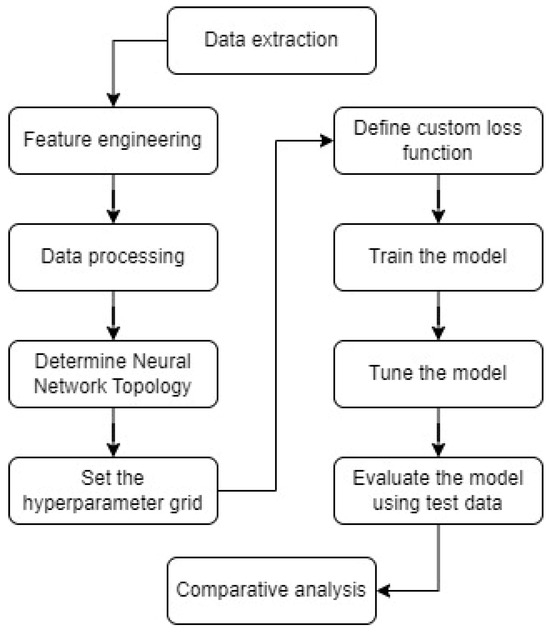
Figure 3.
Framework of the methodology for interval forecasting.
4.1. Feature Engineering
- Time index creation: To capture the temporal trend, a time index was created along with its polynomial terms, such as the square or cube, to model more complex trends. These indices help in identifying underlying patterns over time.
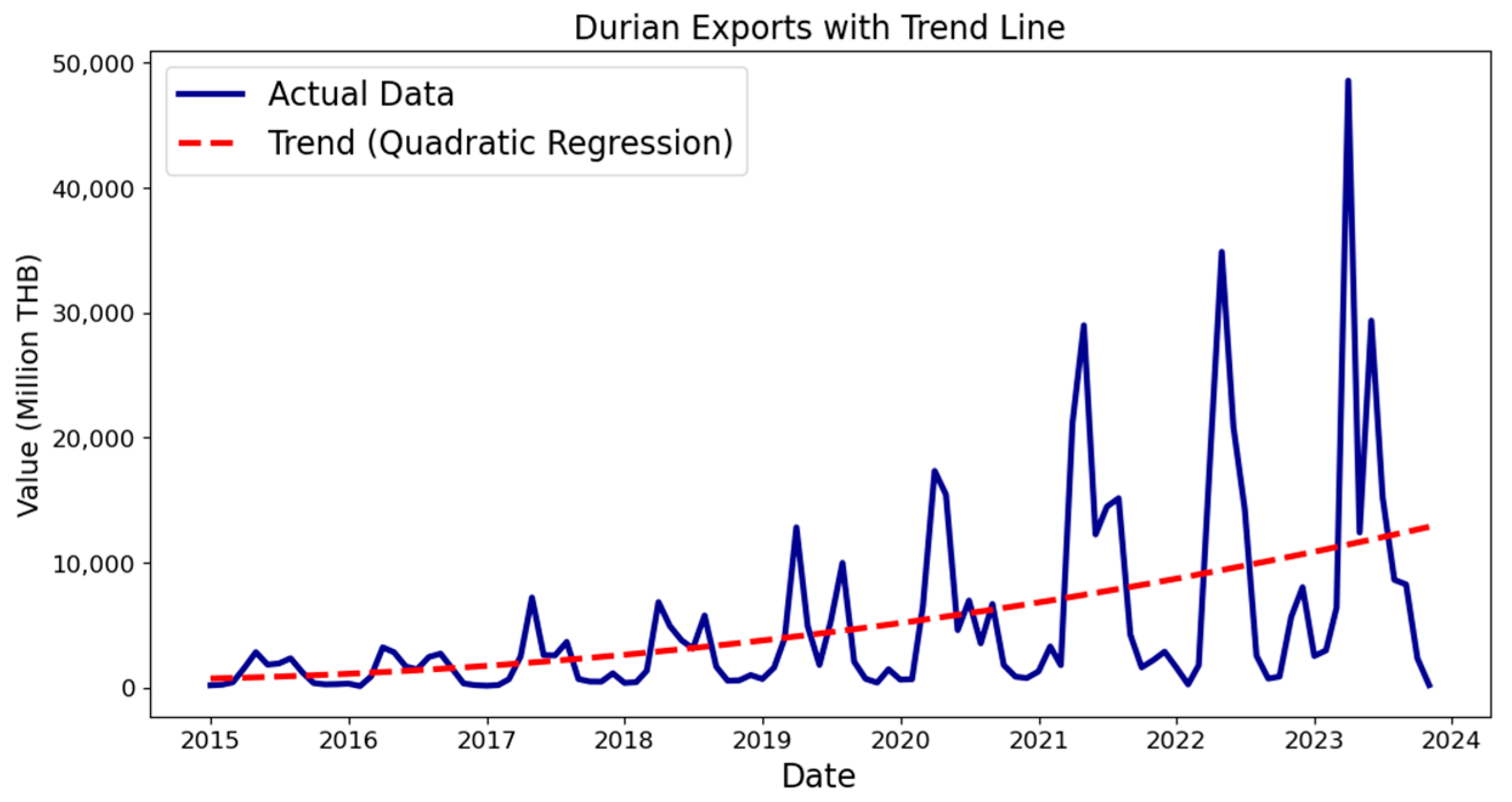
- Quadratic trend estimation: A quadratic regression was fitted to the original data to model the underlying trend and subsequently remove it (detrend), thereby enhancing stationarity. The rationale for choosing a quadratic model is based on the observation that the time-series data for Thailand’s durian export exhibited a quadratic trend. This trend estimation helps in removing long-term trends, making the time series more stationary and easier to model with neural networks. The trend equation is given as the following:where the corresponding trend line is depicted in Figure 4. While a quadratic model was suitable for this specific dataset, the proposed method is not limited to quadratic trends. Other trend models, such as linear, exponential, or higher-order polynomial regressions can be used if they better fit the data.
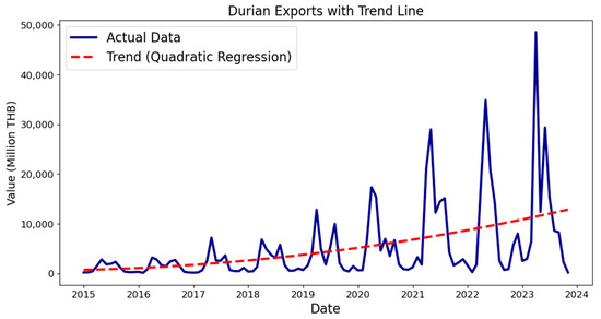 Figure 4. Durian export data with a quadratic trend line.
 - Lag feature generation: Lag features up to 12 months prior were created to incorporate historical data points as predictors. If the data exhibit different seasonal patterns or other temporal dependencies, the lag feature span can be modified accordingly. The proposed method is robust and can adapt to different lag feature configurations to capture relevant patterns in the data.
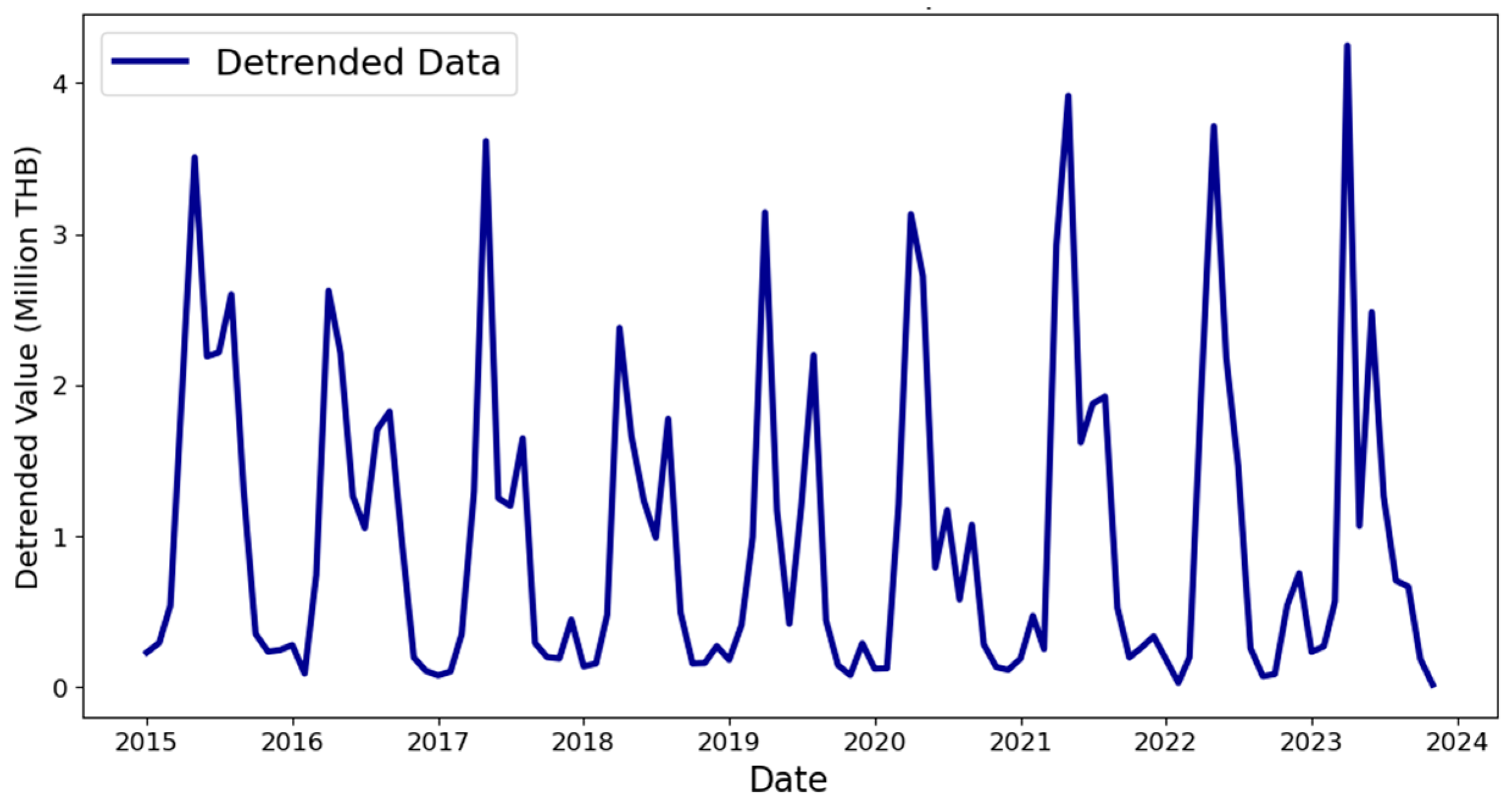
- Detrending: To normalize the time-series data yi, where the model is yi = Ti × Si × Ci × Ii (Trend T, Seasonality S, Cyclical C, and Irregular I), the detrending process involves dividing the original data by the estimated trend:
This normalization results in y/T = S × C × I, removing the long-term trend and making the data more stationary. The detrended data are presented in Figure 5.
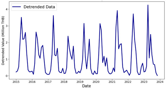
Figure 5.
Detrended durian export.
4.2. Data Processing
- Data cleaning: rows with missing values, resulting from lagged feature generation, were removed to maintain consistency;
- Data splitting: the dataset was split into training and test sets, ensuring a temporal split that mimics real-world forecasting scenarios;
- Feature scaling: the features were standardized using StandardScaler() in Python (version 3.11.5) with scikit-learn (version 1.3.0) to normalize the data, improving the neural network’s convergence.
4.3. Neural Network Topology
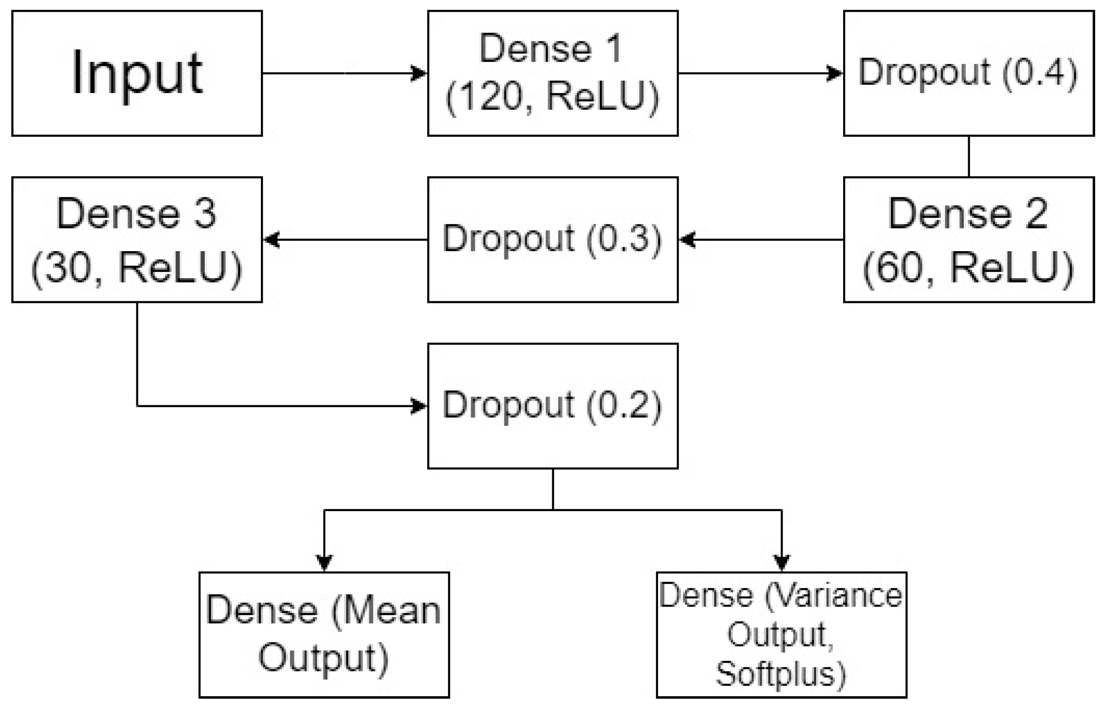
Figure 6 shows one example architecture of the dual-output MCDO neural networks used in this study. It includes an input layer that accepts a feature vector of dimension 12 (corresponding to 12 lagged variables), three dense layers with ReLU activation (120, 60, and 30 neurons), each followed by dropout layers (with rates of 0.4, 0.3, and 0.2, respectively), and branches into two output layers: one for the mean prediction and one for the variance prediction with Softplus activation. This structure can be adjusted to fit different datasets and requirements.
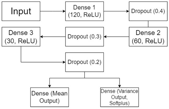
Figure 6.
Example of the neural network architecture of a dual-output MCDO with dropout.
The first dense layer has 120 neurons with ReLU activation, producing a 120-dimensional vector for each instance, calculated as follows:
where and are the weights and biases of the dense layer, respectively, and σ denotes the chosen activation function. The subsequent dropout layer is included to mitigate overfitting by randomly setting 40% (dropout rate of 0.4) of the input units to zero at each update during the training time.
4.4. Hyperparameter Grid
- A minimal multi-layer perceptron (MLP) with a single hidden layer of several neurons (e.g., 10–20) was initially used to establish a baseline. Based on the baseline performance, the network depth was gradually increased by adding more layers and neurons to capture complex patterns. For instance, starting with a two-layer model (60–30 neurons) and then increasing the network depth by adding more neurons (e.g., 120 neurons for three layers, 180 for four, etc.), while carefully monitoring for overfitting. This step-by-step increase ensures that the added complexity is justified by improved performance;
- Different activation functions such as ReLU, Sigmoid, and Tanh were evaluated for their unique characteristics in modeling;
- Dropout, as a method to combat overfitting, involves deactivating a random subset of neurons during each training cycle. Dropout rates were varied across different layers to explore their combined effects. For instance, with a configuration of [0.4, 0.3, 0.2], the first hidden layer uses a dropout rate of 0.4, the second hidden layer uses 0.3, and the third hidden layer uses 0.2. This gradation from 0.2 up to 0.7 allows for a progression from minimal to more intensive regularization, adapting the model’s complexity and preventing it from memorizing the training data too closely. In some experiments, up to five dropout rates were applied at different points in the network to explore their combined effects on regularization;
- Training sessions for the models were conducted over 25, 50, or 100 epochs, where each epoch represents a full pass of the training data through the learning algorithm. Adjusting the epoch count allows the model to refine its grasp on the dataset, though too many epochs can lead to overfitting, where the model too closely adapts to the training data. Conversely, too few epochs may not provide enough learning opportunity, potentially causing underfitting;
- Batch sizes were varied across 16, 32, 64, or 128 to adjust the quantity of data samples processed simultaneously by the network. Opting for smaller batch sizes tends to enhance the stability of the model’s convergence but may prolong the duration of training. Conversely, larger batches expedite the training phase but could compromise convergence stability and the model’s ability to generalize effectively across unseen data.
4.5. Custom Loss Function
Given the predictions ypred, which consist of the mean predictions (μi) and variance predictions (vi), the custom loss function for a single instance is a combination of the mean squared error (MSE) for the mean predictions and a regularization term for the variance predictions. Let ytrue be the vector of true values and be the vector of predictions for the i-th instance. The MSE for the mean predictions is defined as follows:
where refers to the true value for the i-th instance, and μi refers to the predicted mean for the i-th instance. The Softplus function is applied to the variance predictions to ensure they are positive:
The variance regularization term is the mean of the transformed variance predictions:
The custom loss for the batch is the sum of the MSE and the variance regularization term:
where λ is a weighting term to balance the two components of the loss function. This balance ensures that the predicted variance reflects the true uncertainty in the predictions by preventing from collapsing to zero, thus maintaining meaningful variance estimates. The dimensions of ytrue and ypred are not directly comparable, as ypred contains more information (both mean and variance) than ytrue.
4.6. Training Process
- Model compilation and training: Each model configuration from the hyperparameter grid was compiled and trained on the scaled and split training data. The dataset was divided into training (80%) and testing (20%) subsets to ensure proper training and evaluation. Within the training set, a further split was made to create a validation set (20% of the training set), resulting in 64% of the data used for training, 16% for validation, and 20% for testing;
- Validation set evaluation: The validation set (16% of the total data) was used to evaluate the performance of each model configuration. The root mean squared error (RMSE) on the validation set was used as the primary metric to compare different hyperparameter settings. The model configuration with the lowest validation RMSE was selected as the optimal model;
- MCDO for uncertainty estimation: post-training, MCDO was employed to generate predictive distributions by performing multiple forward passes with dropout enabled, aggregating the results to estimate the mean and variance of predictions.
4.7. Tuning of Models
4.7.1. Proposed Method
The proposed method was tuned using a thorough hyperparameter grid search to identify the best combination of hyperparameters. The model configuration with the lowest validation RMSE was selected as the optimal model. The final evaluation metrics, including RMSE, were computed based on this optimized model.
4.7.2. Benchmark Method
The SARIMA model was also tuned to achieve the best performance. The parameters for the SARIMA model were selected using a grid search process similar to the proposed method. The best-performing SARIMA model, based on validation performance, was used for the final comparison.
4.8. Applying Dual-Output MCDO for Interval Forecasting
A dual-output neural network architecture combined with the MCDO methodology is used to forecast durian export values and provide reliable uncertainty estimation. The network employs lagged variables covering a period of 1 to 12 months to account for temporal relationships and seasonal patterns in the data. The results are as follows:
- Mean output: This layer predicts the expected mean value of durian exports for a future time point. The prediction is formulated as , where x represents the input features, including lagged variables, and ΘMean embodies the network’s learned parameters. Dropout introduces a Bayesian approximation;
- Variance output: This layer estimates the predictive variance, which quantifies the aleatoric uncertainty inherent in the data. The estimated variance is
The variance is directly used to create intervals around the predicted mean, using the standard formula for a 95% confidence interval [38]:
Because the MCDO approach can quantify uncertainty by performing multiple stochastic forward passes with dropout, simulating a Bayesian posterior distribution of weights, the predictive distributions for both the means and variances will be graphically presented in the Section 5.
4.9. Evaluation
A comparative analysis will be conducted on the forecast intervals compared to the seasonal autoregressive integrated moving average (SARIMA) model benchmarks. This comparison will use metrics like the mean interval width, coverage proportion, and the incidence rate of non-positive lower limits. When assessing point forecasts, the evaluation will include the root mean squared error (RMSE) and the determination coefficient, represented as R2. The detailed descriptions of these measures are as follows:
- Coverage proportion (%Coverage): This measure indicates the proportion of times the actual values fall within the predicted intervals [39]. It is defined by the following:
- Incidence of non-positive lower limits (%NegLB): This metric calculates how frequently the predicted intervals have a lower limit that is non-positive, which is crucial for datasets where such values are infeasible. It is defined by the following:
- Average width of forecast interval (WidthAvg): Represents the mean distance between the upper and lower bounds of forecast intervals [40]. It is defined as follows:
- Root mean squared error (RMSE): This is a measure of the average discrepancy between the predicted and actual values. It is defined by the following:
- Coefficient of determination (R2): Indicates the fraction of the variance in the observed values that is predictable from the independent variables. It is defined by the following:
- The seasonal autoregressive integrated moving average (SARIMA) model is an extension of the ARIMA model that specifically addresses and models seasonal components of a time series [41,42]. Choosing SARIMA as a benchmark for comparison with proposed forecast intervals for durian export is strategic due to its comprehensive ability to model both seasonal and non-seasonal patterns in time-series data. Elements of SARIMA include non-seasonal (p, d, q) and seasonal (P, D, Q, S) terms, where p and P represent the order of the autoregressive terms, d and D signify the degree of differencing, q and Q denote the order of the moving average terms, and S corresponds to the length of the seasonal cycle. The SARIMA model is defined by the following:
The autoregressive terms ϕ and Φ account for the non-seasonal and seasonal dynamics, respectively. Conversely, the moving average terms θ and Θ address the non-seasonal and seasonal parts. The lag operator L systematically shifts time-series data [43,44,45].
5. Results
The Section 5 is organized into four distinct subsections: the optimization of the dual-output MCDO neural network and the influence of hyperparameters; the predictive distributions of point forecasts; the distributions of forecasted variances; and the comparative analysis of forecast intervals derived from both the proposed method and the SARIMA model.
5.1. Optimal Model and Effects of the Parameters
The optimal model, which achieves the lowest custom loss function as defined in (14), consists of three hidden layers—[p = 30, p = 60, p = 120]—uses the Tanh activation function, and has dropout rates of [p = 0.4, p = 0.3, p = 0.2]. It was trained for 25 epochs with a batch size of 16, resulting in an RMSE of 11,689.41. Under investigation, seven of the ten optimal models have a number of hidden layers not greater than three. This suggests that the deeper dual-output MCDO neural networks experience the overfitting issue. The RMSE of the best 40 models and corresponding hyperparameters are presented in Figure 7.
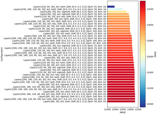
Figure 7.
Top 40 dual-output MCDO neural networks with the lowest RMSE values.
The top 10 optimal MCDO NNs typically feature smaller batch sizes, with the majority employing a batch size of only 16—contrast this with the default value of 32 in the Keras module. The number of epochs commonly ranges from 25 to 50, indicating that a larger count of epochs, such as 100, might not be necessary. It is important to note that the Keras module does not have a default value for epochs; this parameter must be explicitly specified by the user.
Figure 8 shows that models with three layers have the lowest average RMSE, indicating the best predictive performance among the models evaluated. As the number of layers increases or decreases from three, the average RMSE tends to increase, suggesting a decrease in predictive accuracy. Models with four layers exhibit the highest average RMSE, which indicates that additional complexity in this context does not correlate with better performance. Conversely, models with two, five, and six layers show progressively higher RMSEs than the three-layer models, indicating that a medium level of complexity provides a more optimal balance between underfitting and overfitting for the given dataset.
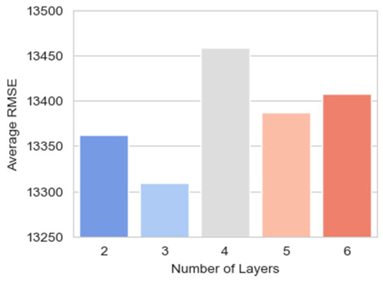
Figure 8.
The number of layers against the average RMSE for models with that specific layer configuration.
Figure 9 presents comparisons of the average RMSE of neural network models utilizing different activation functions: ReLU, Sigmoid, and Tanh. Each bar corresponds to the average RMSE for models employing one of these activation functions. The ReLU has the highest average RMSE among the three. The Sigmoid’s bar is noticeably lower, suggesting better average performance than ReLU. However, it is the Tanh activation function that exhibits the lowest average RMSE of the three, indicating that models using Tanh achieved the best average predictive accuracy in this evaluation.
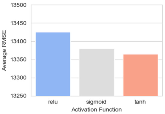
Figure 9.
The average RMSE for models using different activation functions (ReLU, Sigmoid, Tanh).
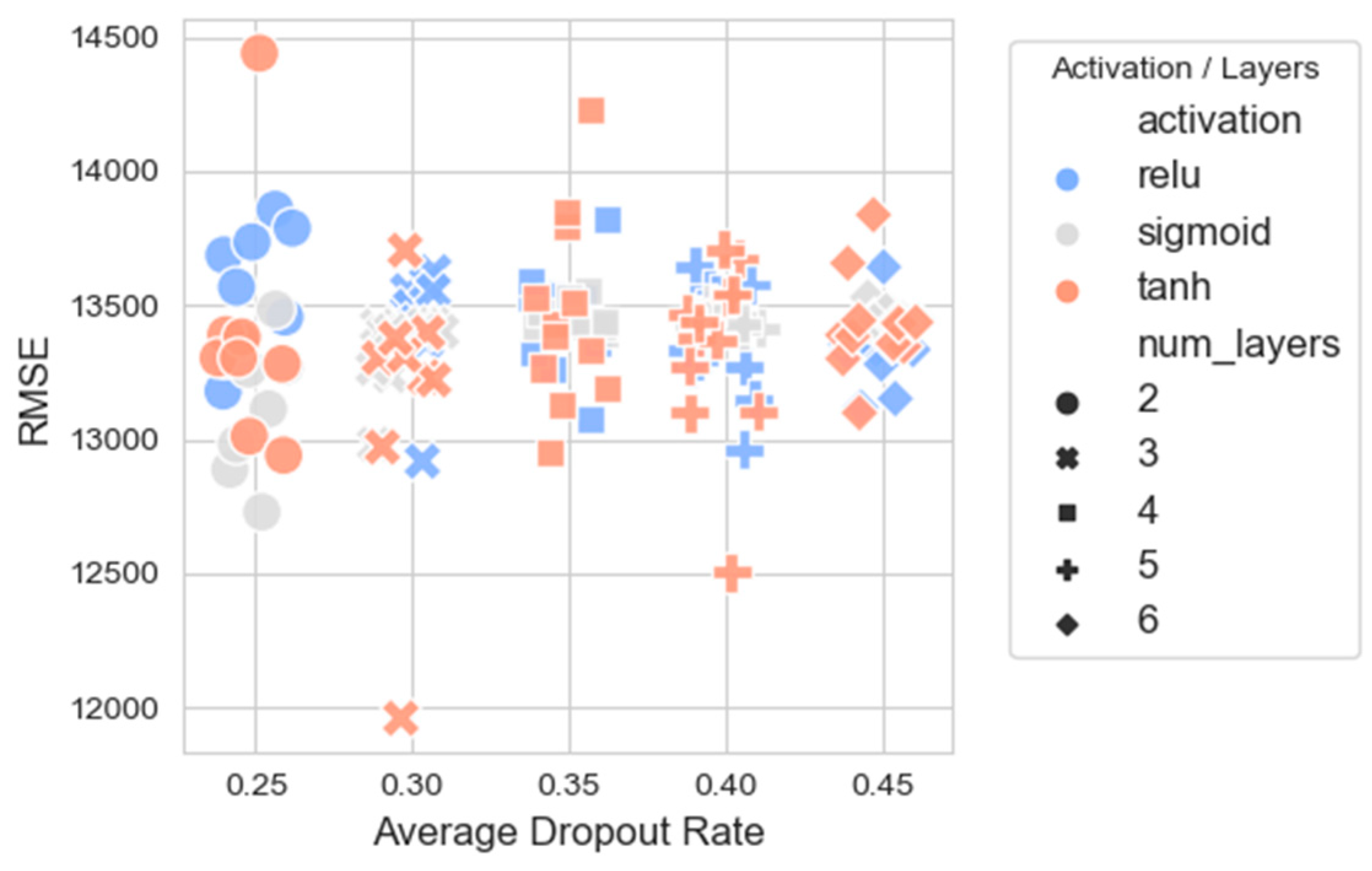
From Figure 10, it is observed that the models with Tanh activation tend to have lower RMSEs across various dropout rates, especially in configurations with three layers, indicating better performance. Models with ReLU activation show a wider spread in RMSE values across dropout rates, suggesting that the performance of ReLU models may be more sensitive to the chosen dropout rate. The Sigmoid activation appears to perform generally in between the ReLU and Tanh models in terms of RMSEs.
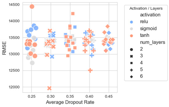
Figure 10.
Scatter plot between the average dropout rate (with added jitter) and the RMSEs of all candidate NNs.
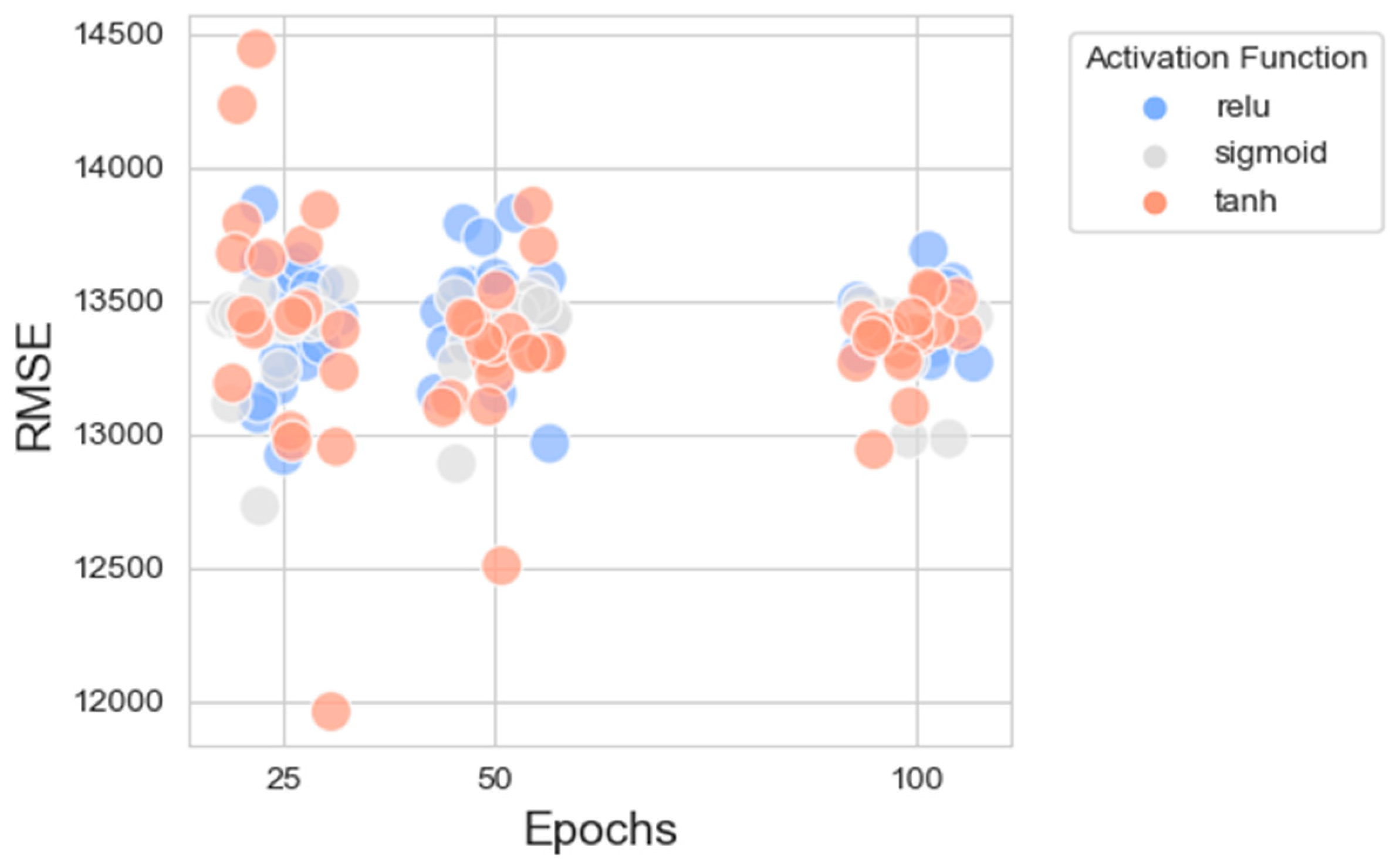
Figure 11 presents a scatter plot illustrating the RMSEs across three distinct epoch values (25, 50, 100) for NNs employing different activation functions. At 25 and 100 epochs, the spread of RMSE values is relatively similar for models using ReLU and Tanh activation functions, with a few models using the Tanh function achieving slightly lower RMSE values. For models trained with 50 epochs, the Tanh activation function seems to result in a slightly lower RMSE when compared to ReLU and Sigmoid, suggesting that Tanh might be more effective, or the models may have converged better at this training length. The variability in RMSE seems to be less for the ReLU activation function, which might indicate a more stable performance or better optimization at this number of epochs compared to the others.
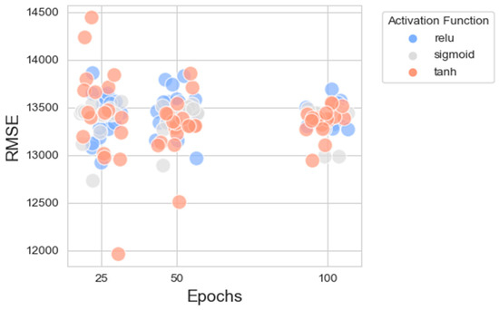
Figure 11.
Scatter plot between the numbers of epochs (with added jitter) and the RMSEs of all candidate NNs.
5.2. Distributions of Forecasting Means
The predictive mean distributions from the optimal dual-output MCDO neural network, as depicted in Figure 12, showcase symmetrical shapes centered around their respective means, indicating a dependable central tendency that is vital for interval forecasting; however, the shapes are not the same. Notably, the distribution for month 1 in the test data (December 2022) is characterized by a narrow, pronounced peak, denoting highly precise predictions, while months 5 and 6 in the test data (April–May 2023) display a broader distribution, suggesting increased predictive uncertainty. month 9 (August 2023) exhibits a slight right skew, which points to the potential presence of outliers. Considering the extensive number of iterations (20,000) and the largely symmetrical shapes of the distributions, the application of normal approximations for the construction of forecast intervals is statistically substantiated.
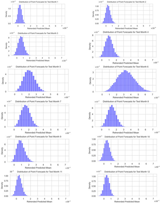
Figure 12.
The predictive mean distributions from the optimal dual-output MCDO neural network for test months 1–12.
5.3. Distributions of Forecasting Variances
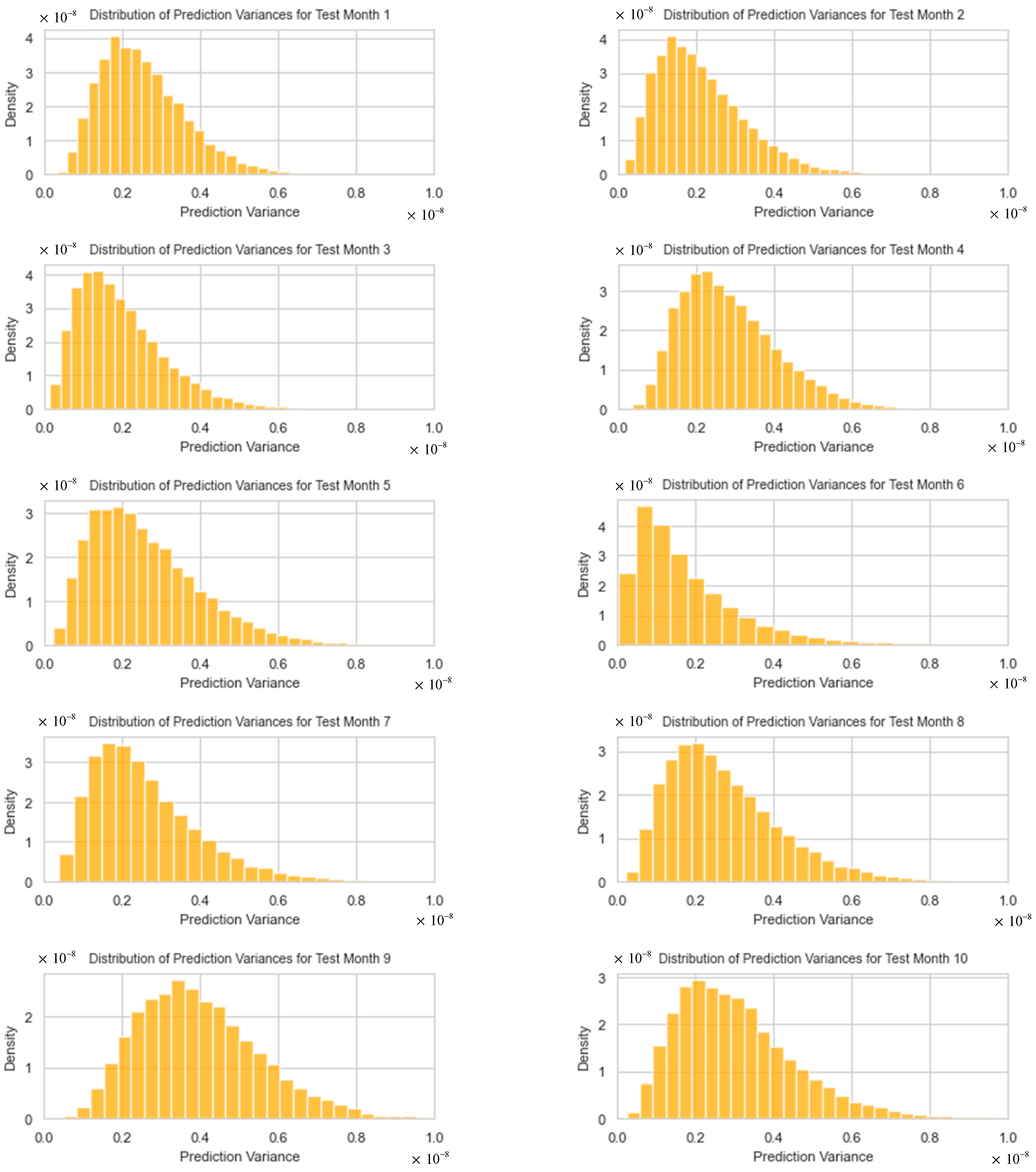
The predictive variance histograms from the optimal dual-output MCDO neural network, as shown in Figure 13, for test months 1 to 12, exhibit a declining trend with variances primarily concentrated toward the lower end. These positively skewed distributions indicate a lower likelihood of very large variances compared to smaller ones. The more concentrated and skewed toward zero these distributions are, the narrower the forecast intervals will be, suggesting higher forecast precision. However, the presence of longer tails, particularly in months 9 to 12 (August–November 2023), points to potential outliers and predicts with less certainty, resulting in wider intervals.
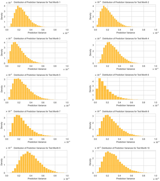
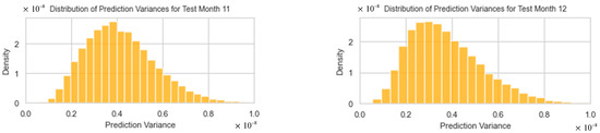
Figure 13.
The distributions of forecasting variances for test months 1–12.
5.4. Forecast Intervals of Durian Export
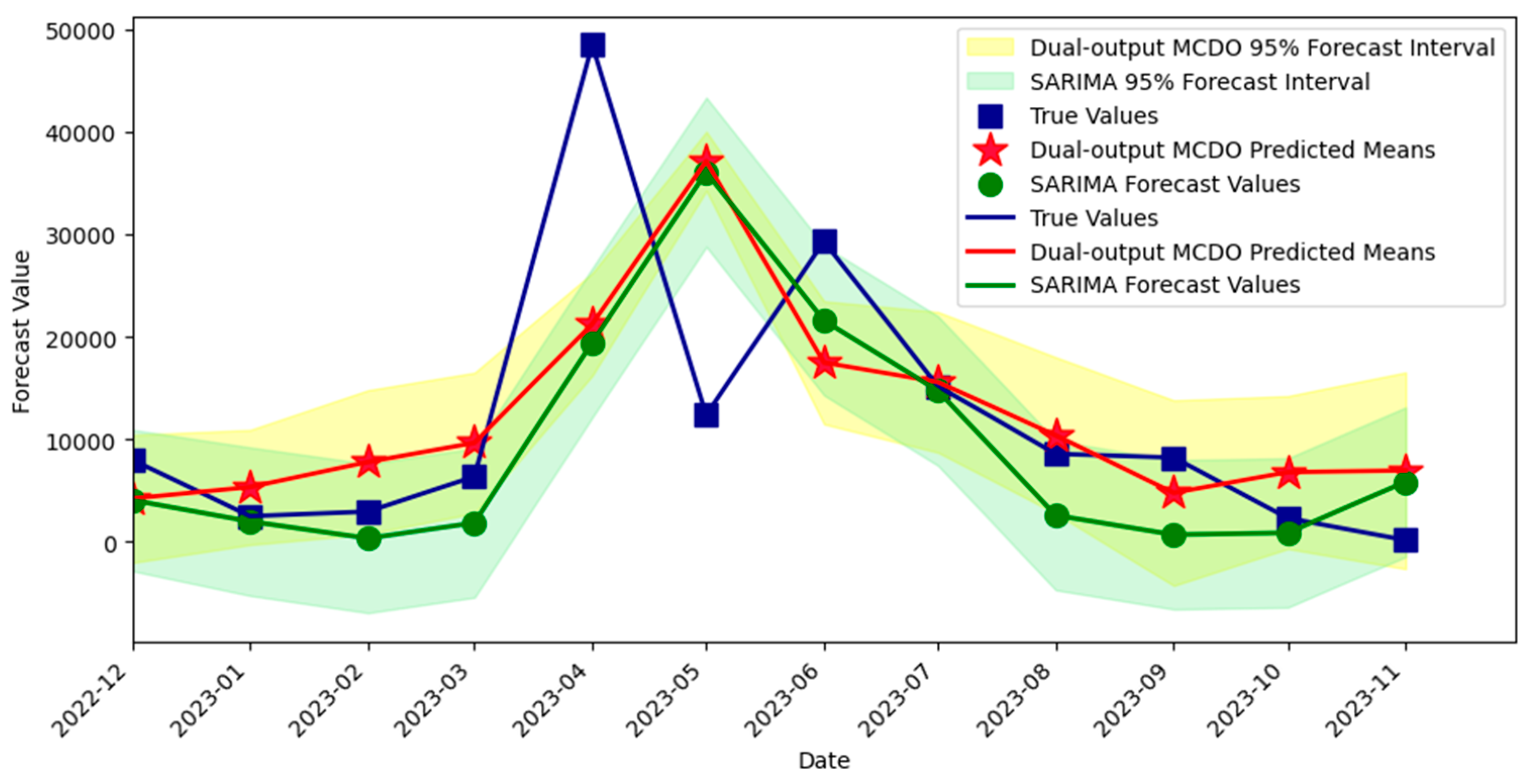
The comparison of the two forecasting methods, spanning from December 2022 to November 2023, is presented in Figure 14. For point forecasts, both models exhibited similar accuracy metrics. The dual-output MCDO NN reported an RMSE of 11,689.40, an MAE of 7974.43, and an R2 coefficient of 0.2297. In contrast, the SARIMA model displayed a comparable RMSE of 11,694.33, a slightly lower MAE of 7772.35, and an R2 value of 0.2290.
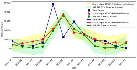
Figure 14.
Forecast intervals obtained from the optimal dual-output MCDO neural network and SARIMA model.
When evaluating the quality of forecast intervals—which is crucial since negative export values are not feasible—the MCDO NN demonstrated superior performance. It achieved a higher coverage proportion of 75%, as opposed to the SARIMA model’s 66.67%. Moreover, the MCDO NN’s intervals were on average narrower, with an average width of 13,373.84, suggesting more precise predictions compared to the SARIMA model’s broader intervals, which averaged 14,514.05. The MCDO NN also exhibited a lower incidence of non-positive lower limits at 41.67% compared to 66.67% for the SARIMA model.
It is noticeable that in test months 5 and 6 (April–May 2023), the point forecasts are not near the true values. This can be explained by Figure 12, where the corresponding predictive mean distributions have heavy tails and more variation than in other test months, indicating high uncertainty for these point forecasts. However, Figure 13 shows that the distribution of forecasted variances for April 2023 (month 5) has a short tail with its mode very near to zero, suggesting that the resulting interval width is expected to be narrower compared to other months.
In contrast, Figure 12 illustrates that in certain months with shorter tails in the distributions, we can anticipate a certain level of accuracy in point forecasting. For instance, in month 1 (December 2022), the distribution appears symmetric and not widely spread. However, the corresponding forecasting variance for month 1, as shown in Figure 13, does not have a mode close to zero, indicating that the interval width might not be as narrow as expected.
6. Conclusions and Discussion
This paper presents an explicit methodology based on a dual-output MCDO neural network for constructing forecast intervals in time-series data, using Thailand’s durian export data as an illustrative example. The methodology effectively captures trends and seasonal patterns while providing comprehensive uncertainty estimates through a Bayesian framework.
The dual-output MCDO model improves forecast accuracy, achieving a lower RMSE compared to traditional models like SARIMA. It handles complex, non-linear relationships and prevents overfitting through dropout techniques. An optimal configuration with three hidden layers, Tanh activation, 25 epochs, and dropout rates around 0.30 was identified through a grid search. The model’s flexibility allows adaptation for different datasets, demonstrating its utility in generating reliable forecast intervals.
However, validating this study on a single dataset may limit the generalizability of the results, particularly concerning the impact of hyperparameters. Additionally, the computational resources required could be substantial, which might constrain its application in some settings.
Future research can apply this methodology to other types of time-series data, refine the hyperparameter optimization process, and integrate additional external variables for enhanced performance. Potential developments include handling multivariate time series, incorporating real-time data updates, and improving computational efficiency to support larger datasets and more complex models. Exploring ensemble methods combining multiple MCDO models could further enhance robustness and accuracy.
Author Contributions
Conceptualization, P.S. and U.K.; Methodology, P.S.; Software, U.K.; Validation, P.S. and U.K.; Formal analysis, U.K.; Investigation, P.S.; Resources, P.S. and U.K.; Data curation, U.K.; Writing—original draft preparation, P.S. and U.K.; Writing—review and editing, P.S. and U.K.; Visualization, U.K.; Supervision, P.S.; Project administration, P.S.; Funding acquisition, P.S. All authors have read and agreed to the published version of the manuscript.
Funding
This study was supported by Thammasat University Research Fund, Contract No TUFT 73/2567.
Data Availability Statement
The data supporting the findings of this study are available from the Office of Agricultural Economics, Agricultural Statistics of Thailand, 2023. These data can be accessed online at https://impexpth.oae.go.th/export (accessed on 15 December 2023).
Acknowledgments
The authors would like to thank the reviewers for their valuable comments and suggestions.
Conflicts of Interest
The authors declare no conflicts of interest.
References
- Gal, Y.; Ghahramani, Z. Dropout as a Bayesian Approximation: Representing Model Uncertainty in Deep Learning. In Proceedings of the 33rd International Conference on Machine Learning, New York, NY, USA, 20–22 June 2016; Balcan, M.F., Weinberger, K.Q., Eds.; PMLR: Westminster, UK, 2016; pp. 1050–1059. Available online: https://proceedings.mlr.press/v48/gal16.html (accessed on 29 May 2024).
- Kendall, A.; Gal, Y. What Uncertainties Do We Need in Bayesian Deep Learning for Computer Vision. In Proceedings of the 31st International Conference on Neural Information Processing Systems, Long Beach, CA, USA, 4–9 December 2017; Guyon, I., Von Luxburg, U., Bengio, S., Eds.; Curran Associates Inc.: Red Hook, NY, USA, 2017; pp. 5580–5590. Available online: https://papers.nips.cc/paper_files/paper/2017/file/2650d6089a6d640c5e85b2b88265dc2b-Paper.pdf (accessed on 29 May 2024).
- Srivastava, N.; Hinton, G.; Krizhevsky, A.; Sutskever, I.; Salakhutdinov, R. Dropout: A simple way to prevent neural networks from overfitting. J. Mach. Learn. Res. 2014, 15, 1929–1958. [Google Scholar]
- Zhang, C.; Sun, S.; Yu, G. A Bayesian network approach to time series forecasting of short-term traffic flows. In Proceedings of the 7th International IEEE Conference on Intelligent Transportation Systems, Washington, WA, USA, 3–6 October 2004; pp. 216–221. [Google Scholar] [CrossRef]
- Pearce, T.; Leibfried, F.; Brintrup, A. Uncertainty in Neural Networks: Approximately Bayesian Ensembling. In Proceedings of the Twenty Third International Conference on Artificial Intelligence and Statistics, Online, 26–28 August 2020; Chiappa, S., Calandra, R., Eds.; Volume 108, pp. 234–244. Available online: http://proceedings.mlr.press/v108/pearce20a/pearce20a.pdf (accessed on 29 May 2024).
- Fortunato, M.; Blundell, C.; Vinyals, O. Bayesian Recurrent Neural Networks. arXiv 2019, arXiv:1704.02798. [Google Scholar] [CrossRef]
- Blundell, C.; Cornebise, J.; Kavukcuoglu, K.; Wierstra, D. Weight Uncertainty in Neural Networks. arXiv 2015, arXiv:1505.05424. [Google Scholar] [CrossRef]
- Srisuradetchai, P.; Lisawadi, S.; Thanakorn, P. Improved Neural Network Predictions with Correlation-Based Subset Selection. In Proceedings of the 2024 12th International Electrical Engineering Congress (iEECON), Pattaya, Thailand, 6–8 March 2024. [Google Scholar] [CrossRef]
- Fan, C.; Zhang, Y.; Pan, Y.; Li, X.; Zhang, C.; Yuan, R.; Wu, D.; Wang, W.; Pei, J.; Huang, H. Multi-Horizon Time Series Forecasting with Temporal Attention Learning. In Proceedings of the 25th ACM SIGKDD International Conference on Knowledge Discovery & Data Mining (KDD 1‘9), Anchorage, AK, USA, 4–8 August 2019; Association for Computing Machinery: New York, NY, USA; pp. 2527–2535. [Google Scholar] [CrossRef]
- Lemay, A.; Hoebel, K.; Bridge, C.P.; Befano, B.; De Sanjosé, S.; Egemen, D.; Rodriguez, A.C.; Schiffman, M.; Campbell, J.P.; Kalpathy-Cramer, J. Improving the repeatability of deep learning models with Monte Carlo dropout. npj Digit. Med. 2022, 5, 174. [Google Scholar] [CrossRef] [PubMed]
- Alahmari, S.S.; Goldgof, D.B.; Mouton, P.R.; Hall, L.O. Challenges for the repeatability of deep learning models. IEEE Access 2020, 8, 211860–211868. [Google Scholar] [CrossRef]
- Hinton, G.E.; Srivastava, N.; Krizhevsky, A.; Sutskever, I.; Salakhutdinov, R.R. Improving neural networks by preventing co-adaptation of feature detectors. arXiv 2012, arXiv:1207.0580. [Google Scholar] [CrossRef]
- Camarasa, R.; Bos, D.; Hendrikse, J.; Nederkoorn, P.; Kooi, E.; van der Lugt, A.; de Bruijne, M. Quantitative Comparison of Monte-Carlo Dropout Uncertainty Measures for Multi-class Segmentation. In Uncertainty for Safe Utilization of Machine Learning in Medical Imaging, and Graphs in Biomedical Image Analysis. UNSURE GRAIL 2020; Lecture Notes in Computer Science; Springer: Cham, Switzerland, 2020; Volume 12443, pp. 32–41. [Google Scholar] [CrossRef]
- Leibig, C.; Allken, V.; Ayhan, M.S.; Berens, P.; Wahl, S. Leveraging uncertainty information from deep neural networks for disease detection. Sci. Rep. 2017, 7, 17816. [Google Scholar] [CrossRef] [PubMed]
- García González, E.; Villar, J.R.; de la Cal Marín, E.A. Time Series Data Augmentation and Dropout Roles in Deep Learning Applied to Fall Detection. In Proceedings of the 15th International Conference on Soft Computing Models in Industrial and Environmental Applications (SOCO 2020), Burgos, Spain, 24–26 June 2020; Springer: Cham, Switzerland, 2020; pp. 563–570. [Google Scholar] [CrossRef]
- Maleki Sadr, M.A.; Zhu, Y.; Hu, P. An Anomaly Detection Method for Satellites Using Monte Carlo Dropout. IEEE Trans. Aerosp. Electron. Syst. 2022, 59, 2044–2052. [Google Scholar] [CrossRef]
- Atencia, M.; Stoean, R.; Joya, G. Uncertainty Quantification through Dropout in Time Series Prediction by Echo State Networks. Mathematics 2020, 8, 1374. [Google Scholar] [CrossRef]
- Sheng, C.; Zhao, J.; Wang, W.; Leung, H. Prediction Intervals for a Noisy Nonlinear Time Series Based on a Bootstrapping Reservoir Computing Network Ensemble. IEEE Trans. Neural Netw. Learn. Syst. 2013, 24, 1036–1048. [Google Scholar] [CrossRef]
- Khosravi, A.; Mazloumi, E.; Nahavandi, S.; Creighton, D.; Van Lint, J.W.C. Prediction Intervals to Account for Uncertainties in Travel Time Prediction. IEEE Trans. Intell. Transp. Syst. 2011, 12, 537–547. [Google Scholar] [CrossRef]
- Murphy, K.P. Machine Learning: A Probabilistic Perspective, 2nd ed.; MIT Press: Cambridge, MA, USA, 2021. [Google Scholar]
- Kingma, D.P.; Welling, M. Auto-Encoding Variational Bayes. In Proceedings of the 2nd International Conference on Learning Representations (ICLR), Banff, AB, Canada, 14–16 April 2014. [Google Scholar]
- Goodfellow, I.; Bengio, Y.; Courville, A. Deep Learning; MIT Press: Cambridge, MA, USA, 2016; Available online: http://www.deeplearningbook.org (accessed on 29 May 2024).
- LeCun, Y.; Bengio, Y.; Hinton, G. Deep learning. Nature 2015, 521, 436–444. [Google Scholar] [CrossRef]
- Glorot, X.; Bordes, A.; Bengio, Y. Deep Sparse Rectifier Neural Networks. In Proceedings of the Fourteenth International Conference on Artificial Intelligence and Statistics (AISTATS), Ft. Lauderdale, FL, USA, 11–13 April 2011; Volume 15, pp. 315–323. [Google Scholar]
- Krizhevsky, A.; Sutskever, I.; Hinton, G. Imagenet classification with deep convolutional neural networks. In Proceedings of the Neural Information Processing Systems (NIPS), Lake Tahoe, NV, USA, 3–8 December 2012. [Google Scholar]
- Polson, N.G.; Sokolov, V. Deep Learning: A Bayesian Perspective. Bayesian Anal. 2017, 12, 1275–1304. [Google Scholar] [CrossRef]
- Bauer, M.; van der Wilk, M.; Rasmussen, C.E. Understanding Probabilistic Sparse Gaussian Process Approximations. In Proceedings of the 30th International Conference on Neural Information Processing Systems (NIPS), Barcelona, Spain, 5–10 December 2016; pp. 1533–1541. [Google Scholar]
- Blei, D.M.; Kucukelbir, A.; McAuliffe, J.D. Variational Inference: A Review for Statisticians. arXiv 2016, arXiv:1601.00670. Available online: https://arxiv.org/abs/1601.00670 (accessed on 29 May 2024). [CrossRef]
- Gal, Y.; Hron, J.; Kendall, A. Concrete Dropout. arXiv 2017, arXiv:1705.07832. Available online: https://arxiv.org/abs/1705.07832 (accessed on 29 May 2024).
- MacKay, D. Probable networks and plausible predictions—A review of practical Bayesian methods for supervised neural networks. Netw. Comput. Neural Syst. 1995, 6, 469–505. [Google Scholar] [CrossRef]
- Murphy, K.P. Probabilistic Machine Learning: Advanced Topics; MIT Press: Cambridge, MA, USA, 2023. [Google Scholar]
- MacKay, D. Information Theory, Inference, and Learning Algorithms; Cambridge University Press: Cambridge, UK, 2003. [Google Scholar]
- Thongkaew, S.; Jatuporn, C.; Sukprasert, P.; Rueangrit, P.; Tongchure, S. Factors affecting the durian production of farmers in the eastern region of Thailand. Int. J. Agric. Ext. 2021, 9, 285–293. [Google Scholar] [CrossRef]
- Rattana-Amornpirom, O. The Impacts of ACFTA on Export of Thai Agricultural Products to China. J. ASEAN PLUS Stud. 2020, 1, 44–60. [Google Scholar]
- Office of Agricultural Economics. Agricultural Statistics of Thailand. 2023. Available online: https://impexpth.oae.go.th/export (accessed on 15 December 2023).
- Kasikorn Research Center. Durian: Record High Export Value of USD 934.9 Million in May 2021. 26 May 2021. Available online: https://www.kasikornresearch.com/en/analysis/k-econ/business/Pages/Durian-z3233.aspx (accessed on 12 November 2023).
- Chaisayant, S.; Chindavong, K.; Wattananusarn, P.; Sittikarn, A. Krungthai Research Note. Krungthai Bank Public Company Limited. 15 May 2023. Available online: https://krungthai.com/Download/economyresources/EconomyResourcesDownload_1938Research_Note_15_05_66.pdf (accessed on 9 December 2023).
- Srisuradetchai, P.; Junnumtuam, S. Wald Confidence Intervals for the Parameter in a Bernoulli Component of Zero-Inflated Poisson and Zero-Altered Poisson Models with Different Link Functions. Sci. Technol. Asia 2020, 25, 1–14. Available online: https://ph02.tci-thaijo.org/index.php/SciTechAsia/article/view/175918 (accessed on 30 May 2024).
- Srisuradetchai, P. A Novel Interval Forecast for K-Nearest Neighbor Time Series: A Case Study of Durian Export in Thailand. IEEE Access 2024, 12, 2032–2044. [Google Scholar] [CrossRef]
- Srisuradetchai, P.; Suksrikran, K. Random kernel k-nearest neighbors regression. Front. Big Data 2024, 7, 1402384. [Google Scholar] [CrossRef] [PubMed]
- Sirisha, U.M.; Belavagi, M.C.; Attigeri, G. Profit Prediction Using ARIMA, SARIMA and LSTM Models in Time Series Forecasting: A Comparison. IEEE Access 2022, 10, 124715–124727. [Google Scholar] [CrossRef]
- Manigandan, P.; Alam, M.S.; Alharthi, M.; Khan, U.; Alagirisamy, K.; Pachiyappan, D.; Rehman, A. Forecasting Natural Gas Production and Consumption in United States-Evidence from SARIMA and SARIMAX Models. Energies 2021, 14, 6021. [Google Scholar] [CrossRef]
- Deretić, N.; Stanimirović, D.; Awadh, M.A.; Vujanović, N.; Djukić, A. SARIMA Modelling Approach for Forecasting of Traffic Accidents. Sustainability 2022, 14, 4403. [Google Scholar] [CrossRef]
- Srisuradetchai, P.; Panichkitkosolkul, W.; Phaphan, W. Combining Machine Learning Models with ARIMA for COVID-19 Epidemic in Thailand. In Proceedings of the 2023 Research, Invention, and Innovation Congress: Innovative Electricals and Electronics (RI2C), Bangkok, Thailand, 24–25 August 2023; pp. 155–161. [Google Scholar] [CrossRef]
- Huadsri, S.; Mekruksavanich, S.; Jitpattanakul, A.; Phaphan, W. A Hybrid SARIMAX Model in Conjunction with Neural Networks for the Forecasting of Life Insurance Industry Growth in Thailand. In Proceedings of the 2024 Joint International Conference on Digital Arts, Media and Technology with ECTI Northern Section Conference on Electrical, Electronics, Computer and Telecommunications Engineering (ECTI DAMT & NCON), Chiang-mai, Thailand, 31 January–3 February 2024; pp. 519–524. [Google Scholar] [CrossRef]


Disclaimer/Publisher’s Note: The statements, opinions and data contained in all publications are solely those of the individual author(s) and contributor(s) and not of MDPI and/or the editor(s). MDPI and/or the editor(s) disclaim responsibility for any injury to people or property resulting from any ideas, methods, instructions or products referred to in the content. |
© 2024 by the authors. Licensee MDPI, Basel, Switzerland. This article is an open access article distributed under the terms and conditions of the Creative Commons Attribution (CC BY) license (https://creativecommons.org/licenses/by/4.0/).