Abstract
Spatial auto-regressive (SAR) models are widely used in geosciences for data analysis; their main feature is the presence of weight (W) matrices, which define the neighboring relationships between the spatial units. The statistical properties of parameter and forecast estimates strongly depend on the structure of such matrices. The least squares (LS) method is the most flexible and can estimate systems of large dimensions; however, it is biased in the presence of multilateral (sparse) matrices. Instead, the unilateral specification of SAR models provides triangular weight matrices that allow consistent LS estimates and sequential prediction functions. These two properties are strictly related and depend on the linear and recursive nature of the system. In this paper, we show the better performance in out-of-sample forecasting of unilateral SAR (estimated with LS), compared to multilateral SAR (estimated with maximum likelihood, ML). This conclusion is supported by numerical simulations and applications to real geological data, both on regular lattices and irregularly distributed points.
1. Introduction
Spatial data are nowadays present in many social and natural phenomena. They are mainly available in two formats: on regular lattices (as digital images and remotely-sensed data), and irregular polygons and sparse points (as in territorial zoning and environmental surveys); see [1] for a detailed description. Spatial data are representable within geographic information systems (GIS) and statistical models may be built for practical purposes, such as filtering and prediction. In digital images, the main goals are denoising and sharpening (e.g., [2]), to perform image segmentation and classification. In polygonal data, the aims are structural analyses and spatial forecasting (e.g., [3]) to support planning decisions.
One of the main features of spatial data is auto-correlation (ACR), which arises from the interaction between random variables located ad different spatial units (pixels in images, and centroids in polygons). The general rule is that the minor is the distance of units, and the greater is the size of the ACR. This dependence must be represented in regression models in order to satisfy the basic assumption of uncorrelated residuals. This, in turn, is necessary to have unbiased and efficient estimates of the parameters and their standard errors; that is, for performing statistical inference and prediction without bias.
On the other hand, ACR is useful for forecasting the character under study in areas where it is not measured, especially when exogenous (X) covariates are not available. It follows that representing the ACR in spatial systems is one of the major concerns of statistical modeling. As in time series analysis, it may be accomplished by introducing into the equations suitable “lagged” terms, i.e., the value of the dependent variable in nearby units. This leads to the spatial auto-regressive (SAR) models, which resemble the AR schemes of time series and dynamical systems. However, while in time there is only a single direction (from past to present), in the plane there are almost infinite directions.
The specification of the models is twofold: unilateral or multilateral, depending on whether the linkage between the nearby units reflects or not a sequential ordering. As an example, in lattice data, one has the triangular and rook schemes in Figure 1a,b [1]; in the first, the dynamic is unidirectional since starting from the upper-left corner it follows the sequence of writing a text [4]. Instead, in Figure 1b the dynamic is multi-directional as each cell involves parts of the text that are not yet written [2]. Figure 1b,c show the analogous situations in polygonal data, where the position of each unit is defined by its center (geometric or political). In Figure 1d the link is multi-directional with four nearest neighbors (NN), whereas in Figure 1c it is in the north direction only.
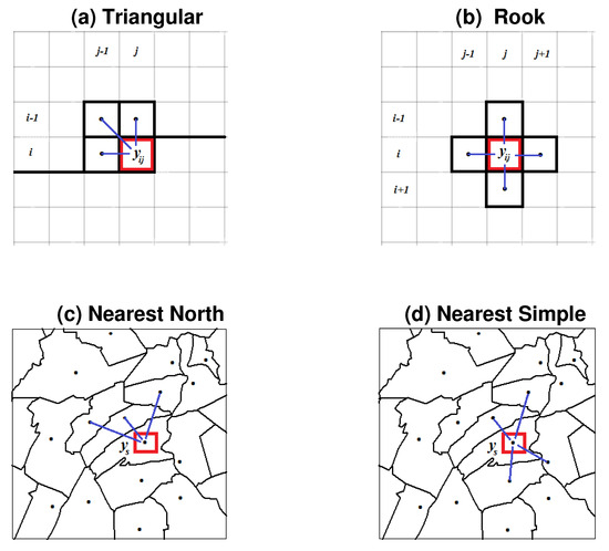
Figure 1.
Examples of lattice (a,b) and polygonal (c,d) data, with unilateral (a,c) and multilateral (b,d) spatial dependence schemes, with respect to their nearest neighbors.
The statistical consequences of the two specifications of SAR models are important. Multidirection linkages violate the condition of independence between regressors and residuals, therefore, making least squares (LS) estimates biased and inconsistent. To solve this problem, many alternative estimators have been proposed, such as maximum likelihood (ML [1,5,6]), generalized method of moments (GM [7]), two-stage least squares [8] and, recently, indirect inference (II [9]). However, these methods are computationally demanding and use iterative algorithms of maximization which may not converge; involve the matrices of spatial contiguity, that must be inverted; require a condition of spatial stationarity (AR parameter ) that may not be fulfilled.
There are also theoretical works that analyze the LS method in multilateral SAR: [10] showed that when the distance among random variables goes to infinity as the spatial dimension increases or the weight matrix converges to zero, then LS is consistent. Ref. [11] investigate the sensitivity of various LS estimators of the AR coefficient using Taylor expansions and find that it is moderate for moderate ACR. Ref. [12] under the null hypothesis, develop refined tests for first-order ACR based on Edgeworth expansion of the LS distribution. Ref. [13] developed an II estimator that implicitly corrects the bias of LS with a mechanism that involves data simulations from a related model; they find that finite sample performance is similar to that of ML. These works show the potential use of the LS method even in SAR models with Toepliz-type contiguity matrices, which are used in social and economic studies.
In this paper, we focus on unidirectional SAR for lattice and polygonal data and we show their ability to preserve the optimal properties of LS estimates even compared to the efficient ML and GM methods. This feature is important because the LS method is linear and can manage datasets of large dimensions, as it may avoid the direct use of the contiguity matrices. Further, unilateral SAR models have a recursive structure, which enables the application of the chain rule of forecasting also outside the observation area. Instead, multilateral SAR models have prediction functions that involve “forward” values and require iterations.
The spatial prediction of missing data (inside the perimeter of the observed area) has been treated by [14,15,16,17] for multilateral SAR models, and [18] in the lattice case. They show that the naive predictor based on the reduced form of SAR systems must be corrected with the best linear unbiased predictor (BLUP) of classical statistics. However, the recursive forecasts of unilateral SAR models do not need this BLUP correction and outperform the others. We show these results with Monte Carlo experiments on synthetic data and out-of-sample forecasting on real data of geosciences, such as digital elevation models (e.g., [19]) and the spatial diffusion of water isotopes (e.g., [20]).
The paper is organized as follows: Section 2 deals with lattice models, it reviews the conditions of identification and consistency and evaluates their forecasts on random surfaces and digital images; Section 3 deals with SAR models for polygonal and sparse point data, it compares the forecasts of unilateral and multilateral models with various algorithms.
2. Regular Lattice Data
Regular lattice data are mostly present in remote sensing and digital images. These data are in the form of rectangular arrays of the type , with , the indexes of position, which may be transformed into latitude and longitude. The values are usually autocorrelated (e.g., clustered) and one of the main goals is to filter the array with its own values, to obtain interpolates and forecasts: . To accomplish this task, SAR modeling puts each cell in relation to the contiguous ones [1,21], such as , where are spatial lags, p is the order of dependence and is an unpredictable sequence.
In time series, the unidirectional (past-present) ordering of data is also called causal and found the analysis of causality between stochastic processes. In lattice data, the causal ordering can be established by following the lexicographic way of reading/writing a text, i.e., processing the cells of starting from the upper-left corner. Unilateral dynamics which satisfy this feature are the row-wise , the half-plane and the one-quadrant (or triangular) with in Figure 1a [2,4]. Although causality is naturally related to the dynamic of events and aspects of human learning, digital filters of denoising and sharpening may follow non-causal models, such as the rook scheme in Figure 1b (e.g., [22]). However, the unidirectional approach remains the favorite solution, because it enjoys properties of sequentiality.
Under linear and unilateral constraints, the triangular SAR(p) model for is defined as follows
with independent normal (IN) residuals. In statistics, the system (1) is usually estimated with the maximum likelihood (ML); this requires the vectorization of the data matrix , of length and the inversion of auto-covariance matrices of size , see [3,23]. This solution is statistically efficient but computationally expensive and can be implemented only for moderate dimensions of the lattice field.
Instead, the LS method can be applied even for large values of ; rewriting the model (1) in regression form as
the LS estimator becomes
The second equation follows from (2) by inserting and is useful for statistical analysis. The linearity of the algorithm (2) can be appreciated with respect to both and the recursive calculation of the sums, see [24]. Unlike the ML approach, it only involves the inversion of a matrix of size , for any value of . The LS estimator is unbiased and consistent for the unilateral model (1) because E.
SAR(1). As an example, let p = 1, then the model (1) is . Applying the formula of [25] to the term , one obtains the moving average (MA) representation
from which E = 0. Similarly, E = because all entries of do not depend on ; hence, the LS estimator (2) is unbiased. This result does not apply to multilateral SAR models, because the MA decomposition would involve ; for the rook scheme in Figure 1b the ML estimator is necessary. Finally, as in a time series, the consistency of LS does not need the stability of the model (1), e.g., ; rather, it improves with the signal-to-noise ratio (e.g., [26]).
SAR(p,q,r). Empirical models often have a subset structure, i.e., have missing lagged terms or they aggregate under a common parameter. The proper definition of such models is SAR(), where p = maximum lag of regressors, q = the number of spatial units and r = the number of parameters. Two parsimonious models that will be extensively applied in the paper are the triangular SAR(1,3,1) and the rook SAR(1,4,1) with drift , defined as
see Figure 1a,b and [1]. These models have almost the same number of regressors and can be written as , where is a local average. The condition of stability in (3) is , because it admits a MA decomposition with weights which converge to 0, see [2]. By analogy, the model (4) is stable if , and this is a necessary condition for the convergence of its ML estimator (see Section 2.1).
2.1. The Vector Form
Previous representations are termed raster in GIS software. When the lattice dimension is moderate (e.g., ), it may be useful to pass at the vector form. Refs. [18,23,25] consider complex forms of vectorization for ML estimation. We follow the spatial econometric approach which vectorizes the data matrix by columns and builds the contiguity matrix of all cells, see [6]. Thus, let of size ; the first-order vector model with drift becomes
where is a unit vector of length N and is an contiguity matrix. Its structure depends on the order p and the marginal values: the models (3), (4) have matrices with sub-diagonals < 1 and sparse 1 on the main diagonal, in correspondence of the border values . For n = 4, m = 7 one has the arrays in Figure 2, see [24]; the distinctive feature of unilateral models is that is always triangular, this provides recursivity to the system.
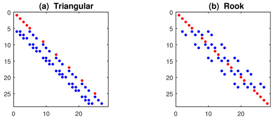
Figure 2.
Contiguity matrices of the models (3), (4) on a lattice of size n = 4, m = 7. Red dots have value 1 and correspond to the border values; while the blue have value 1/3 in Panel (a) and 1/4 in Panel (b); see [24].
The arrays in Figure 2 are obtained by solving the static system , where m determines the number of blocks of size , with matrices at the corners. However, when is inserted in the dynamic model (5), its diagonal elements = 1 must be replaced by 0, obtaining . Each sub-diagonal corresponds to a specific regressor of models (3), (4); thus, the array in Figure 2a can be decomposed as , providing an SAR(3) model. In simulations, the data-generation of proceeds by rows, starting from an initial , as
where is the l-th row of . Unilateral processes are insensitive to , since triangular fills recursively; instead, the model (4), with the forward terms , needs a non-null initial vector, e.g., .
Using matrix algebra, one may obtain the reduced (MA) form of the system (5)
this provides an automatic way to generate SAR data, independent of the initial/border condition . The reduced form (6) is fundamental for ML estimation because, under Gaussianity, the log-likelihood function takes the form
The maximization of Equation (7) proceeds iteratively and requires , i.e., the stability condition , to converge, see [6]. The ML method is compulsory for the rook model (4), but may also be applied to the triangular (3); although LS is preferable (see Table 1).

Table 1.
Performance of LS (8) and ML (7) estimators applied to triangular and rook SAR models (3), (4) with n = m = 32: R-bias = relative bias, R-RMSE = relative root mean squared error, N-test = p-values of the normality test. The bold character indicates the best methods (LS or ML) over model classes (Triang and Rook).
In the vector representation (5), the LS estimator of parameters of the models (3), (4) may use the entire sample as
improving the estimator (2) based on observations. The matrix provides the dispersion of estimates and if is triangular the method is consistent; a formal analysis is in [24].
Spatial Forecasting. Prediction is one of the central goals of SAR modeling; typical examples with lattice data are restoring parts of remote-sensing images hidden by clouds or extrapolating their value outside the observed range. However, existing literature has mostly concerned with in-sample filtering and interpolation, focusing on techniques of image sharpening [22], robust denoising [2] and trend estimation [18], also in conjunction with non-parametric smoothing.
This paper aims to forecast data that are external to the measured perimeter , e.g., on the right-hand side as with or, in vector form on units placed beyond N. By defining the forward indexes, the forecast function depends on the SAR representations, see [15]. Here, we have the lattice form (3), (4), the vector AR (5) and the reduced MA (6); for the triangular model (3), the 3 predictors are
where is the -th row of the augmented matrix and the vector in (10) is updated with the forecasts. The predictor (11) is nearly automatic, but in the absence of exogenous variables provides constant forecasts; on the other hand, the functions (9), (10) need border values to start. These can be set as for all k, and may be improved by r-iterating the forecasts with the nearby values as , etc. This approach can extensively be applied to the rook model (4), with regard to its forward elements ; however, the convergence of , as r increases, is not guaranteed and may give biased forecasts.
The variance of predictors is useful for building confidence intervals and testing hypotheses. A general expression can be obtained for the representations (6) and (11), such as
Finally, in order to compare the models’ performance, a portion of the observed data, e.g., , is excluded from the parameter estimation; then the forecasts of each model are computed and are compared with the mean absolute percentage error (MAPE) statistic
2.2. Simulations and Applications
We develop simulation experiments to test the performance of LS (8) and ML (7) estimators, applied to unilateral and multilateral SAR models. We consider the models (3), (4) with parameters , and border values , i.e., , etc. Data are generated with the reduced form (6), with matrices as in Figure 2 with zero diagonal; 200 replications on a lattice (N = 1024 cells) are obtained with Normal disturbances and . Performance statistics are the relative bias , the relative root mean squared errors (the square root of MSE()/) and the p-values of the Normality test of [27]. Since the relative statistics of do not depend on the parameter size, their value is averaged to provide a single indicator of performance.
The results are displayed in Table 1 and Figure 3; the main findings are as follows: LS (8) is uniformly better than ML (7) when the matrix is triangular. Its efficiency improves as , as a consequence of the super-consistency property of LS estimates in SAR models (e.g., [26]). LS estimates in multilateral SAR models are biased for but still benefit from the super-consistency. Further, unlike time series, the Normal distribution of LS estimates holds even in the presence of the unit root (see Figure 3b).
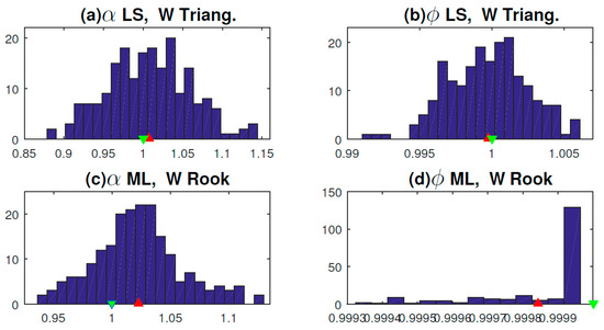
Figure 3.
Distribution of LS and ML estimates in 200 replications of the SAR models (3), (4) with = 1, = 1 (green), and mean values of (red): Panels (a,b) LS (8) of model (3); Panels (c,d) ML (7) of model (4).
Regarding the ML method (7), we used the Matlab implementation of [6], which is computationally demanding. However, it significantly improves the estimates of multilateral models, providing good levels of unbiasedness and efficiency when . On the other hand, it requires conditions of stationarity and its performance in triangular models is disappointing, meaning that ML is mainly designed for sparse-weight matrices. In conclusion, we can state that LS is suitable for unilateral models, whereas ML must be used in multilateral SAR.
We also carry out two applications to test the performance of SAR models in out-of-sample forecasting of lattice data. In comparing predictions, one cannot proceed as in Table 1, because data generated by a certain SAR model will only be better predicted by that model. Hence, we consider data from external sources.
Random Surface. The first application considers rough random surfaces [28]; these models are used in physics to study electromagnetic, fluid and plasma phenomena. We follow an approach based on a fast Fourier transform, where a matrix of random numbers is convolved with a Gaussian filter to achieve a certain spatial autocorrelation. The resulting surfaces are random but smooth and one may add further noise to make them similar to the real data of geostatistics .
Figure 4a,b show an example of and obtained with two Gaussian noises on a 32 × 32 lattice; the computational details are in [24]. The goal is to forecast the last K = 7 columns (about 22%) of the surface with the algorithms (9)–(11). Table 2 reports the in-sample parameter estimates (with LS and ML methods) of the models (3), (4) and their MAPE statistics (12).
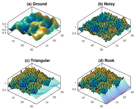
Figure 4.
Panels (a,b): Simulation of a rough random surface of size n = m = 32. Panels (c,d): Out-of-sample forecasts of (:,26:32) with models (3), (4) and predictors (9), (10).

Table 2.
Parameter estimates (with T-statistics in parentheses) of SAR models (3), (4) on the surface (:,1:25) in Figure 4b, and forecast statistics on the data (:,26:32).
A triangular SAR(1,3,3) (with three AR parameters) is also fitted to the data, but it does not improve the forecasts of the constrained (3). However, the best performance is provided by (3) with ML estimates. The rook (4) performs poorly with the (biased) LS estimates, whereas it significantly improves with the ML ones; anyway, the path of the predicted surface in Figure 4d remains disappointing. Ref. [24] provides further results; on 10 replications of the experiment, the mean value of MAPE of (3)-LS is − 37% smaller than that of (4)-ML.
Remote Sensing. The second application regards a real case study; we consider high-resolution elevation data obtained with aerial laser scanners. The sample array comes from USGS [19] and has 340 × 455 pixels (see Figure 5); this would yield a vector SAR model with 154,700 rows. Further, the terrain morphology may require the inclusion of spatial trend components (e.g., [18]), such as bivariate polynomials of degree . Given the numerical issues implied by computing , we only perform analyses with the LS estimator (2); for a model (3) with a quadratic trend, the forecasting function (9) becomes
with , which can be sequentially managed. The AR part of the rook model involves forward values in the lower-right side; however, these may be provided by the polynomial itself: .
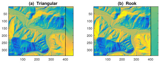
Figure 5.
Application of SAR models (3), (4) with quadratic trend to [19] data: Out-of-sample forecasts of the image portion (:,401:455), displayed in pseudocolor.
In the prediction analysis, we left the right portion of 55 columns (about 12% of the array) as out-of-sample data to forecast. LS estimates of the parameters are reported in Table 3 and graphical results are displayed in Figure 5. Despite the better in-sample fitting (with = 0.977), the rook model has a disappointing performance both in terms of MAPE statistic and visual appearance (see Figure 5b). The reason is partly due to LS estimates of its parameters, with ; however, adjusting their values reduces the MAPE but does not change the (uniform) path of the predicted surface.

Table 3.
LS estimates of SAR models (3), (4) with bivariate polynomials (T-statistics are in parentheses) applied to USGS data [19]: (:,1:400) in-sample, (:,401:455) forecasts.
In real-life applications, where small and inner portions of images must be restored, the spatial polynomials may be fitted locally (around the missing pixels) or may be replaced by nonparametric smoothers (e.g., [18]). In any event, the role of the AR component remains fundamental, as the coefficient is the most significant in both models of Table 3, with a statistic .
3. Point and Polygonal Data
When the data are irregularly distributed in space (either as point processes or polygonal areas), the representation has to change. The spatial process is now defined as ; where the index s also applies to the planar coordinates (latitude and longitude) of the polygon centers (geometric or political), see Figure 1c,d. These variables are irregularly distributed in the plane but have a fixed (non-stochastic) nature; moreover, they may influence the level of the process , according to spatial trends. Thus, the SAR(1) model becomes
where belongs to the unit which is closest to the s-th term, and the vector of regressors may include other covariates.
Unlike the previous section, the adjacency matrix has an irregular structure, which depends on the rule of contiguity. The most common rule is to put each observation in relation to its nearest neighbor (NN) term , according to the Euclidean distance: . Furthermore, under the unilateral constraint, the north/west (NW) → south/east (SE) direction may be followed as in the lattice case. However, polygonal and point data have not lexicographic order; hence, the unilateral constraint may simply be defined along the N-S direction. In this setting, it is useful to order the observations according to the shortest distance from the northern border, i.e., according to the inverse of the latitude . Such ordering may be denoted as or simply , and the model (13) can be written in a sequential form as
where is the north NN of , while the simple NN may be denoted as . As in the lattice case, the property E = 0 is the basis for unbiased LS estimation and forecasting.
As an illustration of NN matrices, we simulate N = 30 random points with and consider q = 3 contiguous terms, see Figure 6. Under the north-south ordering of data, the entries of matrices are concentrated around the (null) main diagonal, and with the unilateral (north) constraint the array is lower triangular. Similarly, to obtain concentrated matrices, ref. [16] ordered the data according to the sum , but they used the simple NN rule. The matrices in Figure 6 provide SAR(3) models but averaged as , they yield constrained SAR(3,1). The analogous model to the lattice model (3) is then
where is the k-north NN of . Instead, in the multilateral model of Figure 1d one has q = 4 and the simple NN terms .
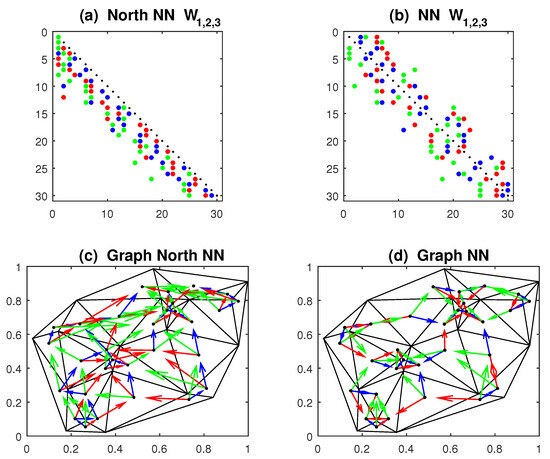
Figure 6.
Contiguity matrices and planar graphs of N = 30 random centroids on the unit square [0, 1], based on nearest neighbors (NN). Panels: (a,c) North NN; (b,d) Simple NN. Matrices: first NN (blue); second NN (red); third NN (green).
Unlike regular lattices, polygonal and point data are not equidistant; therefore, it is useful to consider spatially weighted averages in the model (15). A simple approach is based the inverse distance weighting (IDW)
where is the k-NN of the point . Alternatively, since the inverse distances decay too fast, one can use the exponential weights , with coefficient 0 1. The resulting model is nonlinear and requires complex estimators; however, the value of may be selected a priori and its effect may be evaluated on the LS-ML estimates of .
Models (15) and (16) admit a vector representation (13), with triangular or sparse as in Figure 6. One may also include a lagged term on the exogenous part
this is the Durbin model [6], which is useful when are autocorrelated, i.e., the points have a non-random pattern. The contiguity matrices in Equation (17) may be different, e.g., is preferably triangular, while may be sparse, without affecting the consistency of LS estimates.
3.1. Estimation and Forecasting
The LS estimator of the models (13)–(17) can be obtained from Equation (2) by writing the models in regression form, as , with and , where is an average of q NN terms. In the matrix form (8), the LS estimator of is given by
which can be applied to the Durbin model (17) by including in the term . In the case of triangular , the estimator (18) is unbiased because E by the recursive computation of residuals. In general, under stationarity one can also prove the general result
see [24], where the convergence is in distribution (D).
For non-triangular , the LS is generally biased and one must use ML or generalized moments (GM [7]). The GM solution arises by applying the instrumental variables (IV) method to the LS estimator (18); by using the matrix of instruments , the projection matrix and the modified regressors , the GM estimator is given by . In the numerical section, we compare ML and GM estimators with simulation experiments.
In forecasting, we have L out-of-sample units with value , whose coordinates and regressors are known for all . Their locations may be inside or outside the observed region; in both cases, they are placed at the end of the data matrix . If the data are ordered in a certain direction (e.g., north-south with ), and all L units are outside the observed region, and in the same direction, then the weight matrix is nearly block-diagonal: , where is overlapped to for the contiguity of L target units with the observed ones. In the other cases, it has a more complex structure, with triangular sub-matrices under the unilateral constraint
The forecasting function of depends on the SAR representation used for ; in the reduced (MA) form of (13), the fitted values and the forecasts are jointly computed as
where the joint matrix has q-entries per row and may use non-uniform (IDW) weights. The solution (20) is nearly automatic, but in the absence of exogenous variables, it provides constant forecasts.
The second predictor comes from the structural (AR) representation (13); it is not automatic and must be managed sequentially by rows as
where are the l-th rows of the matrices . Note, that for non-triangular , Equation (21) involves missing values in the running vector . If these values are provided by Equation (20), then the vector of observations and forecasts at the l-th step becomes and in the end , and will only contain the improved forecasts (21).
Refs. [14,17] also discussed solutions based on the best linear unbiased predictor (BLUP) of Goldberger. This approach arises from the conditional mean and variance of Gaussian random vectors:
where is a subvector of the predictor in Equation (20) and come from the partition of the joint covariance matrix of , given by
The conditional variance of the partition of Gaussian vectors also provides the dispersion of the forecasts (22), such as
this matrix requires the error variance , which can be estimated with the in-sample residuals of Equation (20).
3.2. Simulations and Applications
To compare the various estimators, we perform simulation experiments on SAR models (13)–(16) defined on a random grid of N = 150 points, uniformly distributed in the unit square: ∼, as in Figure 6c. We generate the process with an exogenous input , Normal residuals ∼, parameters , contiguity matrices with q = 1, 3 lags and with north NN and simple NN links. Subsequently, M = 500 replications are fitted with LS, ML, GM estimators and relative biases, relative RMSE and p-values of the Normality test were computed for the coefficients and then averaged. Note, that relativization (e.g., bias) allows to combine the statistics of three parameters to have a single indicator of performance.
The results are reported in Table 4, where “variable grid” means that at each replication the centroids change, and “IDW weights” refers to the model (16). The Durbin model includes a lagged term on the exogenous part, as , with coefficients . The software used for ML and GM estimates is the Matlab package of [6], but it does not fit the Durbin model with the GM method. The main conclusions from Table 4 are that ML and GM methods do not improve the LS estimates in the case of unilateral (triangular) matrices. However, they significantly outperform LS in the multidirectional (simple NN) case; in particular, the ML method is the best in terms of MSE. However, these results are not homogeneous regarding unbiasedness and efficiency, and the GM estimator may locally have a smaller bias.

Table 4.
Results of the simulation experiments on the SAR models (13)–(16) with spatial lags
q = 1–3 and single . The statistics are average values (over ) of relative biases, relative RMSE and p-value of N-test. Bold characters indicate the best results.
Forecasting. As in the lattice case, when comparing the predictions of SAR models one must consider data generated from autonomous sources. An idea is to sample the surfaces in Figure 4 at random points ∼∼, and define as the terrain height; however, the forecasting results were too favorable to the unilateral SAR model. We then use the real USGS image in Figure 5, with n = 340, m = 455; we sampled N = 150 pixels and withheld for forecasting L = 30 on the right side, see Figure 7a. We fitted the constrained SAR (15) with q = 3, , triangular and sparse, and forecast functions (20)–(22). The unilateral (west NN) is estimated with LS and the multilateral (simple NN) with ML.
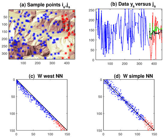
Figure 7.
Graphical results of a single replication of the estimates in Table 5: (a) Random sampling of USGS surface (the points to forecast are in red); (b) Longitudinal display of data and forecasts (21) (unilateral = green, multilateral = black); (c) Contiguity matrix of the unilateral model with q = 3; (d) matrix of the multilateral model (simple NN).
The experiment is replicated M = 100 times (25 in each direction NS, SN, WE, EW, obtained by simply rotating the image ) and the average estimates are reported in Table 5. Both ML and LS estimates detect non-significant spatial coordinates (), which means that the terrain level does not have a (monotone) spatial trend. As in the lattice case, the fitting statistics of the multilateral model are the best, but they are not confirmed out-of-sample. The predictor (21) moderately outperforms the naive (20), with a mild superiority (about 10% on average) of the unilateral model. Notice that the BLUP solution (22) mainly improves the multilateral model, whereas slightly worsens the unilateral one. Figure 7b shows the results of the predictor (21) in a single replication.

Table 5.
Average values, over 100 replications, of parameter estimates (T-statistics are in parentheses), and MAPE forecast statistics of the SAR model (15) on random samples of pixels of the USGS image. Bold character indicates the best results.
As a final application, we consider original point data concerning the measurement of stable isotopes of oxygen (O) and hydrogen (H) in the groundwater. Mapping isoscapes is useful for physical monitoring of the hydrological cycle and for anthropological and forensic investigations, e.g., regarding the path of people’s movement. We consider the datasets of [29], recorded in South Korea in 2010, with N = 130 and [20], recorded in Mexico in 2007, with N = 234. We estimate the SAR model (15) with q = 3 for and = latitude, longitude, to forecast about 20% of observations withheld from estimations. The unilateral constraints of the matrix are south NN for Korea and west NN for Mexico; the results are in Table 6 and Figure 8. They confirm the better performance of unilateral SAR models with the forecast Function (21), especially when the data have significant autocorrelation (i.e., large ) and marked spatial trends (significant ). The reduction in the MAPE statistics in Table 6 ranges from −18% in Korea, to −38% in Mexico.

Table 6.
Parameter estimates (with T-statistics in parentheses) and MAPE forecast statistics of the SAR model (15) with q = 3 applied to the water isotope data of South Korea H (first block) and Mexico O (second block). Bold character indicates the best results.
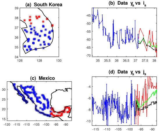
Figure 8.
Water isotope data and SAR forecasts (22): Blue = in-sample data, Red = out-of-sample data, Green = forecasts with triangular; Black = forecasts with multilateral. Panels: (a) South-Korea sample locations; (b) Latitudinal view of Hydrogen isotope; (c) Mexico sample locations; (d) Longitudinal view of Oxygen isotope.
4. Conclusions
In this paper, we have compared unilateral and multilateral SAR models in forecasting spatial data of both lattice and point types. SAR systems are natural extensions of classical autoregressions, their difference is in the treatment of the spatial dependence: while unilateral models choose a single direction in space, as in time series, multilateral models consider multiple directions. These approaches lead to different contiguity matrices: triangular and sparse, usually computed with the nearest-neighbor approach. While triangular SAR can be consistently estimated with least squares, multilateral SARs require maximum likelihood or method of moments; in the latter cases, numerical complexity increases with the dimension of the contiguity matrices. Instead, LS is not sensitive to the size of the lattice or the number of spatial units and can manage even large-scale systems; see the estimator (2). Simulation experiments on small-medium scale systems have shown that ML and GM are suitable for multilateral models, but LS is preferable for unilateral ones, especially in the presence of unstable roots ().
These features can be summarized in Table 7, which are vertically dependent; in fact, the concepts of triangularity, sequentiality, consistency of LS, recursive calculation, chain rule of forecasting, etc., are closely intertwined in the unilateral case.

Table 7.
Summary of the main features of SAR models.
For structural analyses, multilateral models are preferable because the interaction between spatial units does not occur in a single direction. However, structural analyses are mainly concerned with the dependence between the variables ; now, in the Durbin model (17), the matrix may be sparse (for detecting simultaneous relationships), without affecting the properties of unilateral SAR. The role of in structural models is nearly ancillary: it has to remove the ACR of residuals , to have consistent estimates of the standard errors of . It is unlikely that a specific direction, i.e., a particular triangular, may hinder this goal.
Things are different in forecasting, unilateral models with ordered data enable recursive calculations, which allow linear predictions (the chain rule of forecasting). Instead, multilateral models involve forward values which may be pre-estimated only with the (inefficient) reduced form (20) and require iterations. In the applications we have seen that these models benefit from the BLUP improvement (22), but the performance of the unilateral models with the AR predictor (21) remains better, (see Table 5 and Table 6). Regarding the practical usage of SAR point forecasts, we mention the possibility of using them as alternatives to non-parametric smoothers (such as Kriging and Kernels), which are unstable outside the observation perimeter. Further, to overcome the limits of unidirectionality, one can estimate unilateral models in various directions (e.g., NS, SN, WE, EW), and then combine their forecasts with weights proportional to their fitting statistics (e.g., or ). This solution is suitable for points within the investigated area, but can also be applied to external points, by using diagonal paths (e.g., NW-SE).
Funding
This research has not received fundings.
Data Availability Statement
The data are published in the references [19,20,29].
Conflicts of Interest
The author declares no conflict of interest.
References
- Besag, J. Spatial interaction and the statistical analysis of lattice systems. J. R. Stat. Soc. Ser. B 1974, 36, 192–236. [Google Scholar] [CrossRef]
- Bustos, O.; Ojeda, S.; Vallejos, R. Spatial ARMA models and its applications to image filtering. Braz. J. Probab. Stat. 2009, 23, 141–165. [Google Scholar] [CrossRef]
- Barbiero, T.; Grillenzoni, C. Planning a novel regional methane network: Demand forecasting and economic evaluation. Energy Convers. Manag. X 2022, 16, 100294. [Google Scholar] [CrossRef]
- Tjøstheim, D. Statistical Spatial Series Modelling II: Some further Results in Unilateral Processes. Adv. Appl. Probab. 1983, 15, 562–684. [Google Scholar] [CrossRef]
- Anselin, L. Spatial Econometrics. In A Companion to Theoretical Econometrics; Baltagi, B.H., Ed.; Blackwell Publishing: Oxford, UK, 2003; pp. 310–330. [Google Scholar]
- LeSage, J.P.; Pace, R.K. Introduction to Spatial Econometrics; CRC Press, Taylor & Francis Group: Boca Raton, FL, USA, 2009. [Google Scholar]
- Kelejian, H.H.; Prucha, I.R. A generalized moments estimator for the autoregressive parameter in a spatial model. Internat. Econom. Rev. 1999, 40, 509–533. [Google Scholar] [CrossRef]
- Lee, L.F. Best spatial two-stage least squares estimators for a spatial autoregressive model with autoregressive disturbances. Econom. Rev. 2003, 22, 307–335. [Google Scholar] [CrossRef]
- Bao, Y.; Liu, X.; Yang, L. Indirect inference estimation for spatial autoregressions. Econometrics 2020, 8, 34. [Google Scholar] [CrossRef]
- Lee, L.F. Consistency and efficiency of least squares estimation for mixed regressive, spatial autoregressive models. Econom. Theory 2002, 18, 252–277. [Google Scholar] [CrossRef]
- Liu, S.; Polasek, W.; Sellner, R. Sensitivity analysis of SAR estimators: A numerical approximation. J. Stat. Comput. Simul. 2012, 82, 325–342. [Google Scholar] [CrossRef]
- Robinson, P.M.; Rossi, F. Refined tests for spatial correlation. Econom. Theory 2015, 31, 1249–1280. [Google Scholar] [CrossRef]
- Kyriacou, M.; Phillips, P.C.B.; Rossi, F. Indirect inference in spatial autoregression. Econom. J. 2017, 20, 168–189. [Google Scholar] [CrossRef]
- Goulard, M.; Laurent, T.; Thomas-Agnan, C. About predictions in spatial autoregressive models: Optimal and almost optimal strategies. Spat. Econ. Anal. 2017, 12, 304–325. [Google Scholar] [CrossRef]
- Kelejian, H.H.; Prucha, I.R. The efficiencies of various predictors in spatial econometric models containing lags. Reg. Sci. Urban Econ. 2007, 37, 363–374. [Google Scholar] [CrossRef]
- LeSage, J.P.; Pace, R.K. Models for spatially dependent missing data. J. Real Estate Financ. Econ. 2004, 29, 233–254. [Google Scholar] [CrossRef]
- LeSage, J.P.; Pace, R.K. Spatial econometric models, prediction. In Encyclopedia of Geographic Information Science; Shekhar, S., Xiong, H., Eds.; Springer: Berlin/Heidelberg, Germany, 2008; pp. 1095–1100. [Google Scholar]
- Mojiri, A.; Waghei, Y.; Nili-Sani, H.R.; Mohtashami Borzadaran, H.R. Non-stationary spatial autoregressive modeling for the prediction of lattice data. Commun. Stat.-Simul. Comput. 2023, 52, 5714–5726. [Google Scholar] [CrossRef]
- USGS (2017), U.S. Geological Survey, Digital Elevation Models (DEMs). Available online: https://www.sciencebase.gov/catalog/item/543e6b86e4b0fd76af69cf4c (accessed on 1 January 2023).
- Reynaga, D.K.; Millaire, J.F.; Balderas, X.C.; Berrelleza, J.A.; Luján, L.L.; Longstaffe, F.J. Building Mexican isoscapes: Oxygen and hydrogen isotope data of meteoric water. Data Brief 2021, 36, 107084. [Google Scholar] [CrossRef] [PubMed]
- Fingleton, B. Spatial Autoregression. Geograph. Anal. 2009, 41, 385–391. [Google Scholar] [CrossRef]
- Grillenzoni, C. Statistics for image sharpening. Stat. Neerl. 2008, 62, 173–192. [Google Scholar] [CrossRef]
- Awang, N.; Shitan, M. Estimating the parameters of the second order spatial unilateral autoregressive model. Int. J. Stat. Sci. 2006, 5, 37–58. [Google Scholar]
- Grillenzoni, C. Forecasting lattice and point spatial data: Comparison of unilateral and multilateral SAR models. Preprints 2024, 1, 2024080947. [Google Scholar] [CrossRef]
- Basu, S.; Reinsel, G.C. Properties of the spatial nilateral first-order ARMA model. Adv. Appl. Probab. 1993, 25, 631–648. [Google Scholar] [CrossRef]
- Bhattacharyya, B.B.; Richardson, G.D.; Franklin, L.A. Asymptotic inference for near unit roots in spatial autoregression. Ann. Stat. 1997, 28, 173–179. [Google Scholar] [CrossRef]
- Jarque, C.M.; Bera, A.K. A test for normality of observations and regression residuals. Int. Stat. Rev. 1987, 55, 163–172. [Google Scholar] [CrossRef]
- Sheffield, S. What is a random surface? In Proceedings of the International Congress of Mathematicians 2022, Virtual, 6–14 July 2022; International Mathematical Union, EMS Press: Philadelphia, PA, USA, 2022. [Google Scholar]
- Gautam, M.K.; Song, B.-Y.; Shin, W.-J.; Bong, Y.-S.; Lee, K.-S. Datasets for spatial variation of O and H isotopes in waters and hair across South Korea. Data Brief 2020, 30, 105666. [Google Scholar] [CrossRef] [PubMed]
Disclaimer/Publisher’s Note: The statements, opinions and data contained in all publications are solely those of the individual author(s) and contributor(s) and not of MDPI and/or the editor(s). MDPI and/or the editor(s) disclaim responsibility for any injury to people or property resulting from any ideas, methods, instructions or products referred to in the content. |
© 2024 by the author. Licensee MDPI, Basel, Switzerland. This article is an open access article distributed under the terms and conditions of the Creative Commons Attribution (CC BY) license (https://creativecommons.org/licenses/by/4.0/).