Article

Granger Causality-Based Forecasting Model for Rainfall at Ratnapura Area, Sri Lanka: A Deep Learning Approach

by
Shanthi Saubhagya
1,*,
Chandima Tilakaratne
1,*,
Pemantha Lakraj
1 and
Musa Mammadov
2
1
Department of Statistics, University of Colombo, Colombo P.O. Box 1490, Sri Lanka
2
School of Info Technology, Faculty of Science, Engineering and Built Environment, Geelong Waurn Ponds Campus, Deakin University, Geelong P.O. Box 423, Australia
*
Authors to whom correspondence should be addressed.
Forecasting 2024, 6(4), 1124-1151; https://doi.org/10.3390/forecast6040056
Submission received: 8 August 2024 / Revised: 12 October 2024 / Accepted: 14 October 2024 / Published: 29 November 2024
(This article belongs to the Section Weather and Forecasting)

Abstract

:
Rainfall forecasting, especially extreme rainfall forecasting, is one of crucial tasks in weather forecasting since it has direct impact on accompanying devastating events such as flash floods and fast-moving landslides. However, obtaining rainfall forecasts with high accuracy, especially for extreme rainfall occurrences, is a challenging task. This study focuses on developing a forecasting model which is capable of forecasting rainfall, including extreme rainfall values. The rainfall forecasting was achieved through sequence learning capability of the Long Short-Term Memory (LSTM) method. The identification of the optimal set of features for the LSTM model was conducted using Random Forest and Granger Causality tests. Then, that best set of features was fed into Stacked LSTM, Bidirectional LSTM, and Encoder-Decoder LSTM models to obtain three days-ahead forecasts of rainfall with the input of the past fourteen days-values of selected features. Out of the three models, the best model was taken through post hoc residual analysis and extra validation approaches. This entire approach was illustrated utilizing rainfall and weather-related measurements obtained from the gauging station located in the city of Ratnapura, Sri Lanka. Originally, twenty-three features were collected including relative humidity, ssunshine hours, and mean sea level pressure. The performances of the three models were compared using R M S E . The Bidirectional LSTM model outperformed the other methods (RMSE < 5 mm and MAE < 3 mm) and this model has the capability to forecast extreme rainfall values with high accuracy.

1. Introduction

Background

Weather is important in many aspects of human life. It influences decisions in agriculture, food production, hydropower generation, traveling, and transport. Adversely, it brings forth sudden life-threatening disaster situations such as droughts, floods, extreme rainfall, and pandemics [1,2,3,4]. Occasionally, some of these weather-driven events appear as a chain of events. For example, long-term warm weather increases the level of evapotranspiration which often leads to heavy or extreme rainfall. The chain can end up triggering a flash-flood event [5,6,7,8,9,10]. Proactive reactions to this unbreakable natural chain can be executed by making accurate forecasts of these weather patterns.
Among weather prediction studies, rainfall forecasting is critical and challenging due to its intervention in sequential disastrous events, and difficulty in producing more accurate forecasts with adequate lead time [11]. Due to inherent uncertainty in rainfall fluctuations, a substantial research gap has been created in capturing its extremely rare events, called extreme rainfall events [2,12,13,14,15].
Moreover, rainfall is interconnected with many weather and meteorological variables like relative humidity, mean sea level pressure, sunshine hours, cloud cover, wind speed, and temperature patterns [1,4,16]. The complex relationships among these variables make the selection of the best set of predictor variables for a rainfall forecasting model more critical [13].
Past studies reveal that rainfall forecasting is conducted by predicting rainfall occurrence at a certain location, e.g., [2,4,9,17] or obtaining forecasts for future rainfall for a particular timestep, e.g., [1,3,6,7,8,10,18,19]. For both types of studies, researchers have used various and different structures of predictor variables. In addition to the conventional numerical approach, some studies have been supported by weather-related radar and image data, e.g., [2,9,17].
Building a model for accurately forecasting rainfall, most importantly extreme events, is catalyzed by an effective selection of input features, e.g., [1,2,3,4,5,6,7,8,9,10,11,12,13,14,15,16,17,18,19,20,21,22,23,24,25,26,27,28]. Selecting an appropriate set of features leads to a parsimonious model and prevents over-fitting data [29,30]. This can be conconducted using many approaches such as Random Forest Feature Section, Lasso, Principal Component Analysis, Correlation Coefficient, Information Gain, Sequential Forward and Backward Selection, and Genetic Algorithm [30]. These approaches are categorized under filters, wrappers, and embedded algorithms methods [29,30,31]. Past studies further point out that embedded algorithms like Random Forest are an intermediate solution between filter and wrapper methods [30]. Many studies which describe applications in different areas such as global warming, genetic population assignment, network security, and cancer diagnosis (e.g., [32,33,34,35,36]) have used Random Forest to identify the best set of features for their models and gained better performances than standalone approaches. Though the Pearson Correlation Coefficient is widely used (e.g., [37,38,39,40,41,42]) as a feature selection method, it is limited to the selection of predictor variables which are linearly related with the response variable without making any adjustment of other exogeneous variables.
As a causality dependence approach, recently, the Granger Causality test has gained much attention among researchers to identify the best set of input features to models. The review in [43,44,45,46,47,48] emphasizes the applications of the Granger Causality technique in addressing specific causality problems in the climate system. Due to its strength in identifying the predictor variables which show a significant impact on the response variables, we applied the Granger Causality test to identify predictor variables to the rainfall forecasting model. However, only the non-categorical predictor variables can be chosen from this technique. Therefore, the Random Forest technique was adopted aiming to identify suitable categorical predictor variables.
As mentioned in the recent study [9], many researchers have attained better forecasts of rainfall by employing machine learning or deep learning methods, including K-Nearest Neighbor (KNN), Random Forest, Artificial Neural Network (ANN), and Convolutional Neural Network (CNN). Nowadays, deep learning models are being vastly applied to develop forecasting models, including rainfall forecasting models (e.g., [49,50,51,52,53,54,55,56]). Hybrid models such as CNN-LSTM are also becoming popular in weather forecasting. For example [14], used hybrid models to combine ground-level weather variables and satellite images, and obtained an accuracy of 75% in short-term rainfall forecasting. The literature (e.g., [18,57,58,59,60,61] reveals that LSTM is the most popular model that is used for rainfall forecasting. Different versions of LSTM, such as Bidirectional LSTM and LSTM Autoencoder-based models [49,57,62] were applied by past studies. In accordance with past studies, we also adopted three types of LSTM versions: Stacked LSTM, Bidirectional LSTM, and Encoder-Decoder LSTM. These models facilitate sequential modeling of inputs and outputs of time series.
Obtaining accurate forecasts for extreme events is another key concern as sequential input-output modeling of the time series. Extreme rainfall events are complex, hazardous, and costly, and their frequency and intensity are reported to be increasing [7,13,27]. Thus, there is a crucial need to identify such events as early as possible, probably, at least one day in advance to warn relevant vulnerable groups of individuals [8,11]. The study in [11] identified the nonlinear relationship between global Sea Surface Temperature (SST) and extreme precipitation through the Distance Correlation-Pearson Correlation method to extract key inputs from SST to feed into the Random Forest model for forecasting monthly extreme precipitation. The resultant model had an R2 value of 0.81 and relatively small R M S E and M A E values.
Different configurations of LSTM were applied to model extreme rainfall with 12 isobaric pressure levels and surface data from meteorological stations in Brazil’s southeastern region. The study incorporated a mechanism for dealing with imbalanced data found in rainfall data. With the input of the past 24 h to obtain 6 h ahead forecasts, the model came up with better results: an M A E of 6.9 mm and R M S E of 6.94 mm [13]. Another application of deep learning to forecast extreme rainfall occurrence was found in study [28]. Initially, the Stacked Auto-Encoder (SAE) model was conducted for feature extraction, and then the reduced features were used for classification with Cost-sensitive Support Vector Machine (SVM). The proposed model was capable of predicting extreme rainfall events 6 to 48 h before their occurrence, even though it resulted in several false positives. The study further highlights the difficulty in predicting such events 1 to 2 days earlier, and the importance of accurate early predictions in avoiding vast damages. The study in [63] used six extreme rainfall indices including the 90th percentile of rain day amounts (mm/day) and greatest 5-day total rainfall (mm) as factors in the Back Propagation Neural network model with stepwise regression to forecast the average extreme rainfall in the coming year. Nonetheless, the study claims that the model’s accuracy is not satisfactory and needs to be further improved. Another drawback of this model is that it does not provide the exact day or time when extreme rainfall happens, i.e., annual average extreme rainfall will not be sufficient to mitigate harmful consequences. These past studies stress the essential need of finding more sophisticated methods for accurate modeling of extreme rainfall. Our study also emphasizes obtaining accurate forecasts of extreme rainfall, as the identification of extreme rainfall in advance will help to plan disaster mitigation actions. Unlike past studies, our study attempts to forecast extreme rainfall events in a considerably longer period ahead, probably 3 days-ahead. Such a longer forecast horizon is essential to implement necessary disaster mitigation actions.
Ratnapura in Sri Lanka is severely affected by floods almost every year. It is situated in the wet zone of the country and receives heavy rain during south-west monsoon periods. Due to its geographical location and the nature of the Kalu River which passes through the area, Ratnapura experiences floods almost every year and sometimes more than once a year. Further, most of the existing global weather forecasting systems (e.g., Google Weather Forecasting System and MSN Weather Forecast) only provide the chance of having precipitation in the said area. Nonetheless, the intensity of the rainfall is necessary to decide the continuation of the day-to-day tasks, as well as to predict future devastating events like floods. Therefore, building a rainfall forecasting model that is capable of identifying accurate extreme rainfall in Ratnapura, at least a few days ahead, is vital.
Among the limited number of published studies that aimed at forecasting rainfall in different locations of Sri Lanka, only a few studies are related to the Ratnapura area (e.g., [2,64,65]). The study described in [2] forecasted the occurrence of rain in selected weather stations including Ratnapura station with the help of Markov models. The study conducted in [64] forecasted rainfall of the Wet and Dry zones of Sri Lanka based on regression techniques and the authors of the study included the rainfall of Ratnapura Station when modeling rainfall of the Wet Zone. Annual rainfall of Ratnapura was forecasted based on mathematical models in [65]. None of the aforementioned studies applied deep learning models for building forecasting models nor paid special attention to forecast extreme rainfall with high accuracy. Though [64] reduced the dimension of the input variables through Principal Component Analysis, an attempt was not taken to identify an optimal set of input variables. None of the other studies also paid attention to selecting a suitable set of predictor variables. Our study attempts to fill this gap by applying suitable techniques to identify an optimal set of predictor variables.
Considering the importance of obtaining accurate rainfall predictions including extreme events through effective feature selection, and the research gap found in the application of such a model to vulnerable areas like the city of Ratnapura in Sri Lanka [2,9,66,67], this study presents a two-way feature selection method to identify the best set of variables for rainfall modeling with deep learning. More importantly, this study incorporates spatial dependencies into the forecasting model by including a predictor variable representing the rainfall of neighboring stations. The model developed in this study forecasts rainfall with higher accuracy, notably extreme rainfall. This is very important for developing countries like Sri Lanka where agriculture has become one of the major sources of income for the citizens, and often seeks ways and means to reduce the significant allocation of budget for disaster management activities [68,69].
The rest of the paper is organized as follows. The next section explains the feature selection methods and deep learning approach used in modeling rainfall. The Results and Discussion section summarize the key findings and limitations. The last section provides the conclusion and proposes future research directions.

2. Materials and Methods

2.1. Data and Data Pre-Processing

The target or dependent variable of the study is the daily precipitation data collected for the Ratnapura rainfall gauging station located in Sri Lanka with longitude, latitude coordinates of (80.40, 6.680). The potential predictor variables include relative humidity (day/night), temperature (maximum/minimum), mean sea level pressure (morning/evening), wind speed (morning/evening), wind direction (morning/evening), cloud amount (morning/evening), dew point (morning/evening), evaporation, sunshine hours, Nino index, and southern oscillation index (SOI). To capture the spatial impact, rainfall of six neighboring gauging stations, namely, Balangoda (St1_Bal), Detanagalla (St2_Det), Elston (St3_Els), llumbuluwa (St4_Ill), Keragala (St5_Ker), and Moralioya (St6_Mor) were also considered for the study. Spatial interpolation was computed by applying the spatiotemporal kriging method [9] on daily rainfall gathered from these six stations, and rainfall estimates taken from satellite image modeling were also included as potential predictor variables. Additionally, three new variables generated using existing precipitation data from the target station, accumulated rainfall, consecutive dry days, and consecutive wet days, were also added to the list of potential input variables. Altogether, there were 23 potential predictors. The study covered the data from the period of 1 January 2015–31 December 2019.

2.2. Feature Selection and Model Building

Selection of input features to the forecasting model is vital as the accuracy of forecasted value heavily depends on the input features. The study applied two feature selection methods. First, the Random Forest model was developed using all potential predictor variables and obtained feature importance. Starting from the least important feature, the backward elimination approach was conducted to rebuild Random Forest models with reduced features. The features of the model which produced the best performance were extracted. Secondly, the Granger Causality test was applied to all pairs of time series variables consisting of the dependent variable and each potential non-categorical predictor variable. By this process, the non-categorical input features which show a significant impact on the dependent variable were identified as suitable input features to the forecasting model. Through this dual feature selection approach, it was expected to select the lagged values of the non-categorical predictor variables identified by the Granger Causality tests together with the lagged observations’ categorical predictors obtained by the Random Forest model as the optimal feature set to feed into the final rainfall model. However, none of the categorical variables were selected by the Random Forest model. Therefore, only the sets of features suggested by Granger Causality tests were fed into the three LSTM models, Stacked LSTM, Bidirectional LSTM, and Encoder-Decoder LSTM. Based on the performances of the three models, the best method was selected for forecasting rainfall values at Ratnapura.

2.2.1. Random Forest Regression

Random Forest is known as a supervised ensemble learning method which can be applied for both classification and regression [70]. In the regression problem, it constructs a multiple of independent regression trees with controlled variation, and each tree in the ensemble is trained on a different subset of the training data. The selection of the subset is performed with replacement, and this method is as popular as bagging or bootstrap aggregating [9,71]. Then, it makes its own independent prediction. The final prediction is obtained based on the average or weighted average of all the individual predictions of regression trees.
Another important aspect of Random Forest is the two measures it generates as end results, the importance of the features, and the internal structure of the data (the proximity of different data points to one another). When estimating the importance of a feature, Random Forest determines how much prediction error increases when data for that feature is dropped while all other features are kept unchanged [72].

2.2.2. Granger Causality Test

The bivariate Granger Causality was first defined by C. W. J. Granger [73], by building a causal model between two jointly covariance stationary time series, X t and Y t . The simple idea behind the causality test is that the time series X t is causal for the other time series Y t if knowledge of the past history of X t is useful for explaining the future state of Y t over and above knowledge of the past history of Y t itself. If the prediction accuracy of Y t is significantly improved by including lag variables of X t as predictors in the model, then X t Granger causes Y t [46,47].
The simple causal model of x ( t ) and y ( t ) can be defined as:
y t = i = 1 p m a x α i     y t i + i = 1 p m a x β i     x t i + ε t  
where α and β are regression coefficients that can be determined from the data by using ordinary least squares method,   ε t is the error term at time t , and p is the lag length varies from 1 to a maximum value p m a x which is finite and less than the size of the given time series.
To test whether X t causes Y t , a restricted form of Equation (1) is estimated eliminating X t . This is conducted by setting β in Equation (1) to zero.
y t = i = 1 p m a x α i     y t i + ε i  
Then, to test whether the restricted form in Equation (2) is significantly different from the unrestricted form in Equation (1), the F ratio is calculated as follows:
F X t ~ Y t = ( S S E r S S E u r ) / H S S E u r   / ( n K )   ~   F H ,       n K
where S S E r and S S E u r are sum of squared errors with respect to the models given by Equations (2) and (1), respectively, H is the number of coefficients set to zero in the restricted form, K is the number of predictors in the unrestricted form, and n is the number of observations.
If F X t ~ Y t > F α % ,   H ,   n K , then, the null hypothesis of the predictor variable, X t does not Granger cause the variable, and Y t is rejected. It indicates that X t Granger causes Y t .

2.2.3. Long Short-Term Memory (LSTM)

Recurrent Neural Network (RNN) is a supervised deep learning model which contains a recurring connection in each unit of the hidden layer that is interconnected in every different time [3]. LSTM, which is an extension of the RNN, overcomes the vanishing gradient problem often faced by RNN. It is also effective in capturing long-term dependencies. It has four layers interacting in a very special way. The memory cell consists of a forget gate, input gate, and output gate [9,74].
As illustrated in Figure 1, the output of the last moment and current input value are fed into the forget gate to obtain the output, f t at the forget gate:
f t = w f   . h t 1 ,   x t + b f
where f t 0 ,   1 , w f is the weight at forget gate, b f is the bias at forget gate, x t is the current input value, and h t 1 is the output at previous moment. Then, the same previous output and current input value are inputted to the input gate to find the output value. The candidate cell state at the input gate is as follows:
i t = w i   . h t 1 ,   x t + b i
C ~ t = t a n h w c   . h t 1 ,   x t + b c
where i t 0 ,   1 , w i is the weight at input gate, b i is the bias at input gate, w c is the weight at candidate input gate, and b c is the bias at candidate input gate. Then, the current cell state is updated as depicted in Equation (7).
C t = f t C t 1 + i t C ~ t
In order to obtain the output O t at the output gate, h t 1 and x t are fed into output gate at time t (Equation (8)).
O t = w o   . h t 1 ,   x t + b o
where w o is the weight at output gate and b o is the bias at input gate. Finally, the output of the LSTM is computed with the current cell state and output at the output gate as below:
h t = O t t a n h C t
The Stacked LSTM, Bidirectional LSTM, and Encoder-Decoder LSTM are extensions of Vanilla LSTM (with a single hidden layer of LSTM units). The Stacked LSTM has multiple hidden LSTM layers where each layer contains multiple memory cells. This makes a more ideal representation of sequence data, and therefore works more effectively [75,76]. The Bidirectional LSTM learns the input sequence for both forward and backward directions and concatenates both interpretations. The Encoder-Decoder LSTM is especially designed to address the sequence-to-sequence or seq2seq problem [77].

2.2.4. Model Evaluation

The evaluation of Random Forest Regression and LSTM models were conducted using the performance metrics of Root Mean Squared Error ( R M S E ) and Mean Absolute Error ( M A E ).
The computation of R M S E and M A E was conducted as shown below [78].
R M S E = 1 n   i = 1 n y a i y ^ p i 2
M A E = 1 n   i = 1 n y a i y ^ p i
where y ^ p i is the predicted value and y a i is the actual value at the time point i . The smaller the values of R M S E and M A E the better the accuracy of forecasted values is. All the models were fitted using Python 3.10 and run in Google Colab.

3. Results and Discussion

3.1. Feature Selection

The importance of all the aforementioned 23 potential input variables were tested through a two-way feature selection process to get rid of the curse of dimensionality in LSTM modeling. With the reduced feature modeling, it is expected to obtain an efficient model in forecasting rainfall at Ratnapura.

3.1.1. Modeling with Random Forest Regression

Initially, the past three days’ values of the potential predictor variables were modeled with the current day rainfall amount at Ratnapura with Random Forest Regression. The training set includes 80% of the data while the test set consists of the last 20% of the data.
For the full model with all potential predictor variables, the feature importance was obtained, and based on the importance score, feature ranking was established (see Table A1 in Appendix A). Then, the backward elimination approach was used to re-model the Random Forest Regression Tree with the reduced feature. The feature or the potential predictor variable with the lowest rank, i.e., the least important feature, was eliminated first in building the second regression tree. This process continued until the model consisted of one predictor variable which was the most important. The tunned model parameters are listed in Table 1, and the performances of the built models are tabularized in Table A2.
Since the performances of the models with varying numbers of predictor variables fluctuated with slight differences, the model with the best set of features was difficult to identify. Thus, the most important 15 predictor variables were considered to proceed with the study. However, none of the categorical variables are included in this subset of input variables.

3.1.2. Granger Causality Test Results

As a thorough verification of potential input features, bivariate causality was checked between the time series of rainfall at Ratnapura and each potential input variable except the categorical predictors including wind direction (morning/evening).
The results from the Granger Causality test indicated that mean sea level pressure (morning/evening), southern oscillation index, and wind speed (morning/evening) did not show any causal effect on the rainfall at Ratnapura during the study period. The predictors that showed a significant causal effect on the rainfall at the target station and number of significant lags are summarized in Table 2.
As depicted in Table 2, the significant past lag range was different for each causal feature. When incorporating past lags of the selected features to final rainfall modeling, selecting the farthest lags may not add a significant amount of information to the model, especially when conducting the short-term rainfall forecasting [79,80]. It will also increase the complexity of the model, thereby reducing computational efficiency. It is worth noting that our study concerns the short-term rainfall forecasting at Ratnapura. The Granger Causality test results show less than 14 significant lags for some predictor variables and more than 14 lags for other predictors. Therefore, considering these matters, a two-week period of data (i.e., 14 past lags) was taken as a moderate length of historical values from all the predictive features to be input as final sequential inputs to the LSTM rainfall models. As LSTM itself chooses optimal weights for inputs, feeding 14 past lags of predictive features to LSTM will not degrade the performance of the forecasting model. Further, the rainfall forecasts from this network model are intended to be used as input values for our following study on flood forecasting. This model is also a concern of short-term forecasting. The preliminary study on flood occurrence at Ratnapura confirmed that the rainfall of the recent previous days (mostly the past 03 days) greatly impacts flood occurrence in the next day. Therefore, 3 days-ahead outputs or rainfall forecasts were obtained in our study.

3.2. Rainfall Modeling with LSTM Models

Three different LSTM models, Stacked LSTM, Bidirectional LSTM, and Encoder-Decoder LSTM were employed to identify the better model in producing 1 to 3 days-ahead rainfall forecasts at Ratnapura with the inputs of the past 14 days-values of extracted 14 optimal predictive features. Therefore, the set of inputs to the model and obtaining predictions for the next three days’ rainfall values as outputs from the model were the same for all the three utilized models. The training was conducted with moving windows with the selected data which resulted in a size of a 14 × 14 matrix (14 variables × 14 lags). The data from 1 January 2015 to 31 December 2018 were taken for the training and daily data of the year 2019 were used for the testing purpose. The data from the said period was considered to exclude the periods with sequential missing values of rainfall series.
The comparison of the performance of the three models is summarized in Table 3 and Table 4, and the common parameter settings of those models are presented in Table 5.
When selecting the best model, 1st to 3rd days-ahead forecasts only for the periods 1–31 January, 1–31 May, 1–31 August, and 1–30 November 2019 (which represent dry, moderate and extreme rainfall seasons) obtained from the three models, were compared. When obtaining the forecasted values, for instance, firstly the forecasted rainfall of 1–3 January 2019 was obtained by feeding the input values corresponding to the immediate past 14 days to the trained models. Secondly, the forecasted rainfall of 2–4 January 2019, was obtained using the input values corresponding to the past 14 days from 1st January backward as illustrated in Figure 2. This procedure was repeated until the forecasted rainfall of the last 3 days of the testing period was obtained. With respect to RMSE and MAE values, the best fit was selected to obtain forecasts for the rest of the days in 2019.
Table 3 presents the R M S E and M A E values obtained when applying the three selected LSTM models on the four testing periods selected. The results evidence that the Bidirectional LSTM model has outperformed the other models in each step and each month of the forecast. Further illustrating, it can be explained that the aforementioned model holds the lowest R M S E and M A E values in forecasting each upcoming day’s rainfall value when compared to the other two models.
Furthermore, a summary of forecasting actual rainfall events as No or Mild Rain (≤12.5 mm), Moderate Rain (>12.5 mm and <100 mm), and Extreme Rain (≥100 mm) were obtained and are depicted in Table 4. Both the correctly forecasted counts and percentages (within parentheses) are given. In setting the above cut-off values, the definition of light rain and heavy rainfall by the Meteorology Department of Sri Lanka was taken into consideration.
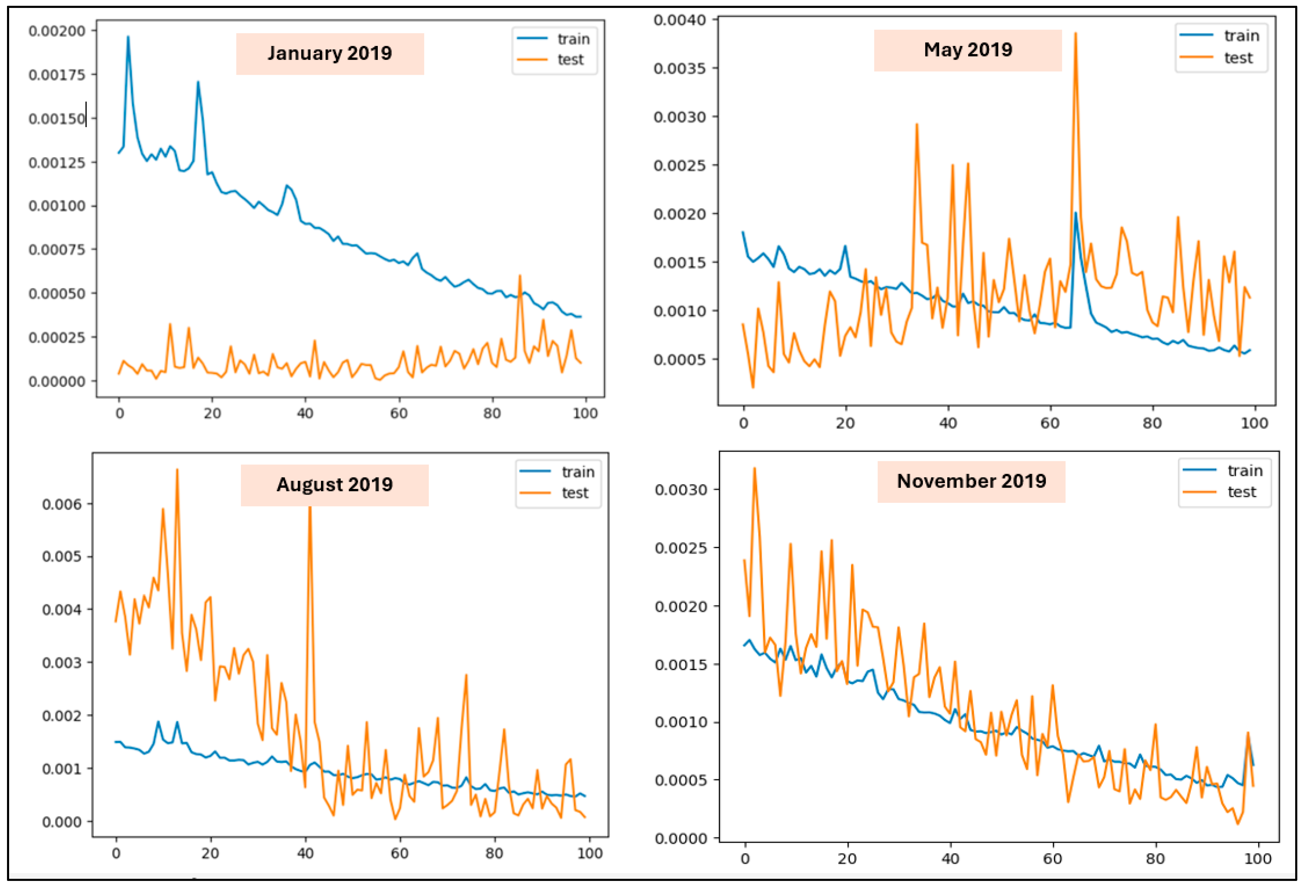
Moreover, the training loss and validation loss of the Bidirectional LSTM Model for January, May, August, and November in 2019 were separately plotted to diagnose the behavior of the model (see Figure A1 in Appendix B). The figure showed that the model has not under- or over-fit the data.
The above results confirm the capability of the Bidirectional LSTM model in rainfall forecasting at Ratnapura, especially the extreme rainfall events. Therefore, the model was further used to forecast the rainfall at Ratnapura for the rest of the period (1 February 2019–24 December 2019).
The sequential model was run in GPU of Google Colab. Since the model was trained with moving windows, training was not computationally efficient. Therefore, the prediction has to be conducted monthly-wise in Colab to avoid the kernel becoming interrupted in the middle of the training. Moreover, the aim was to build a less complex model.
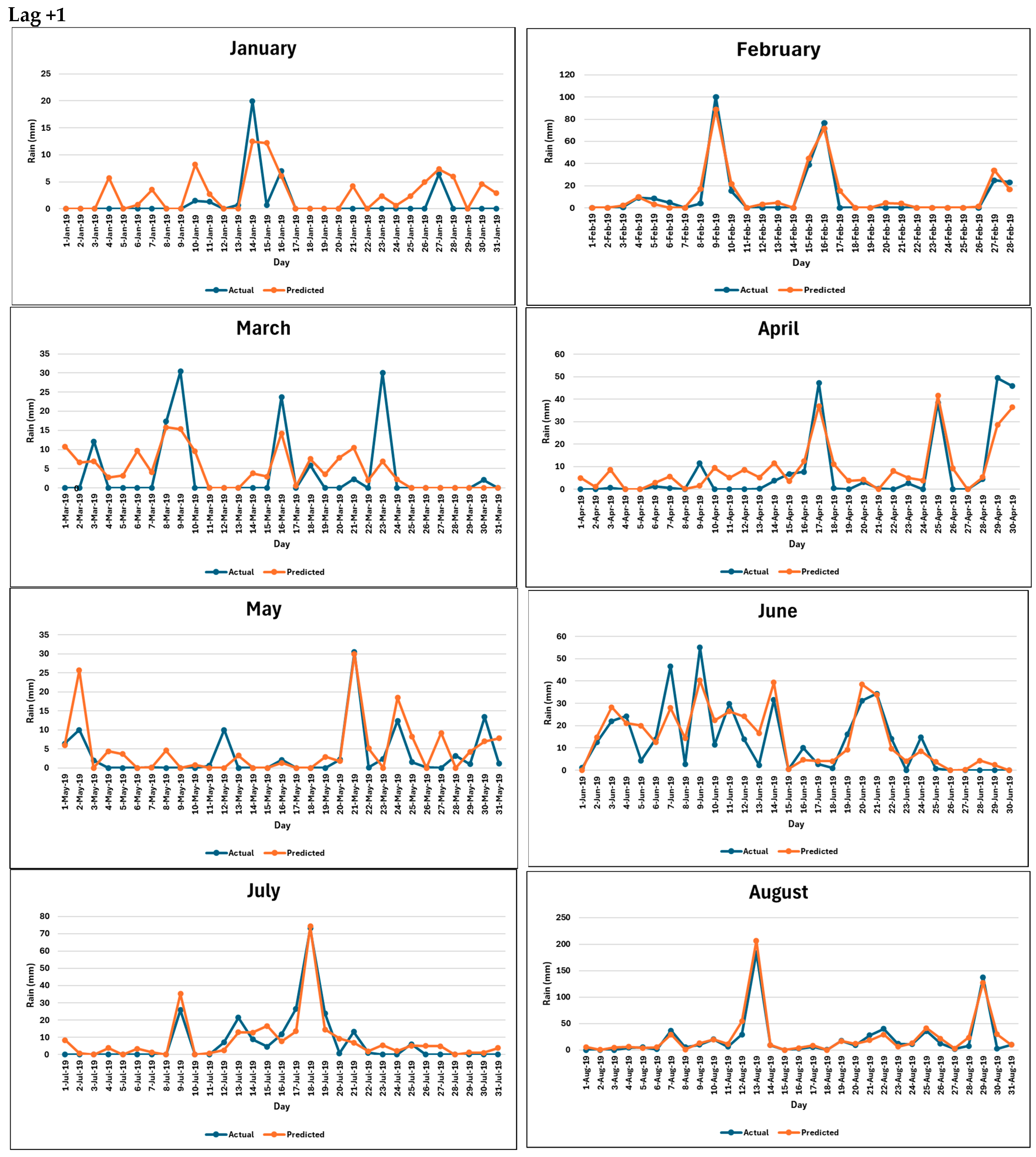
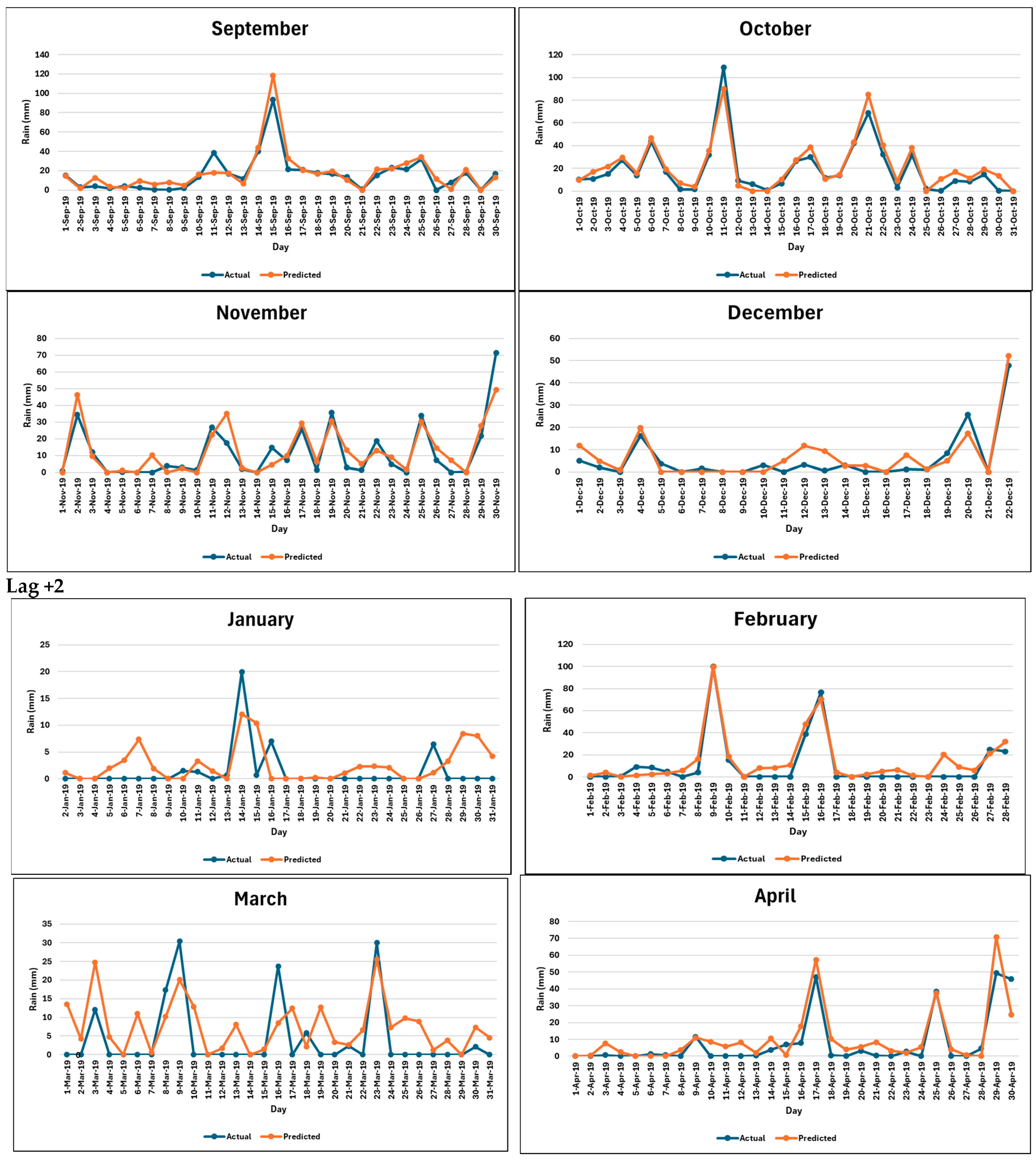
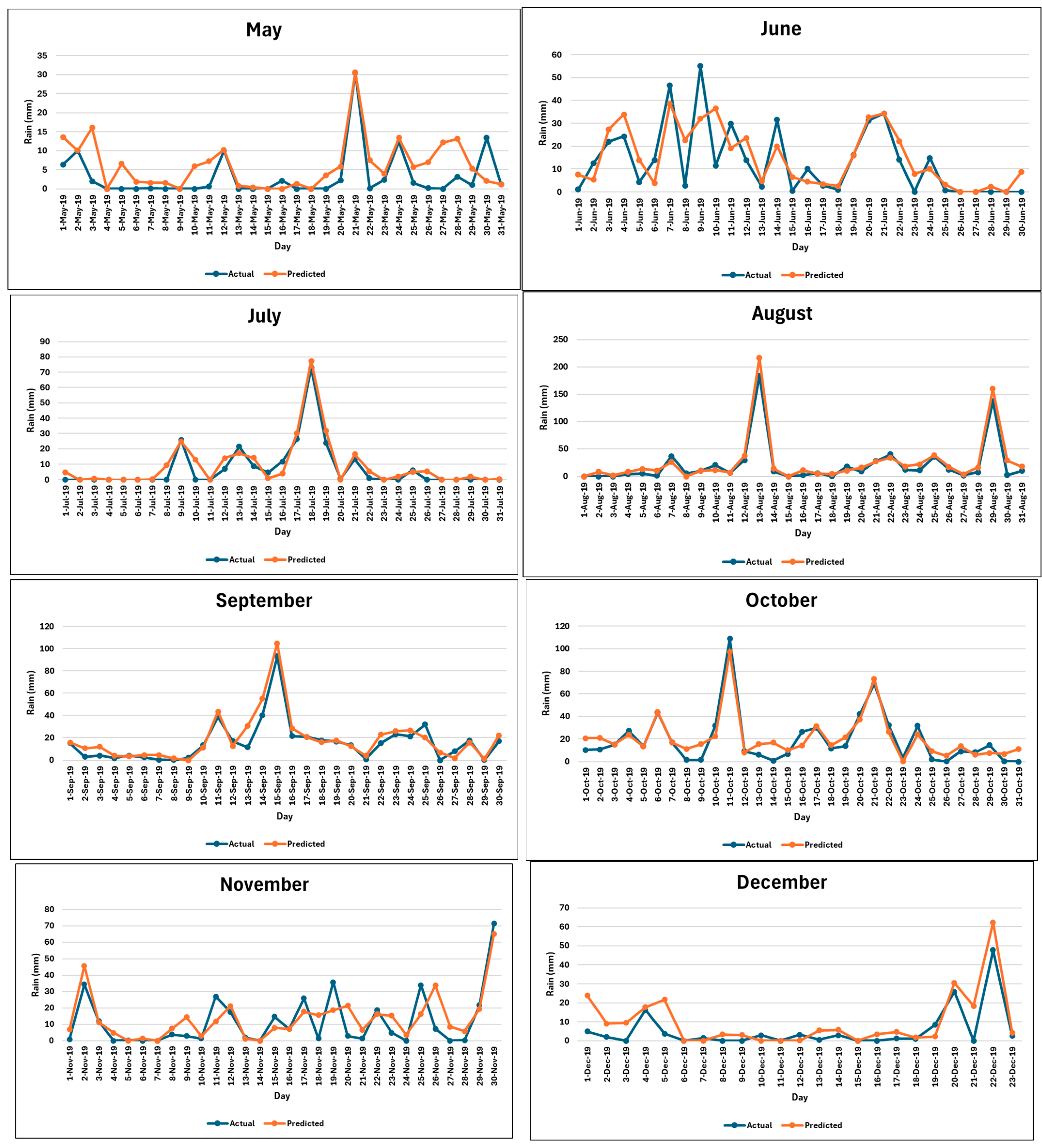
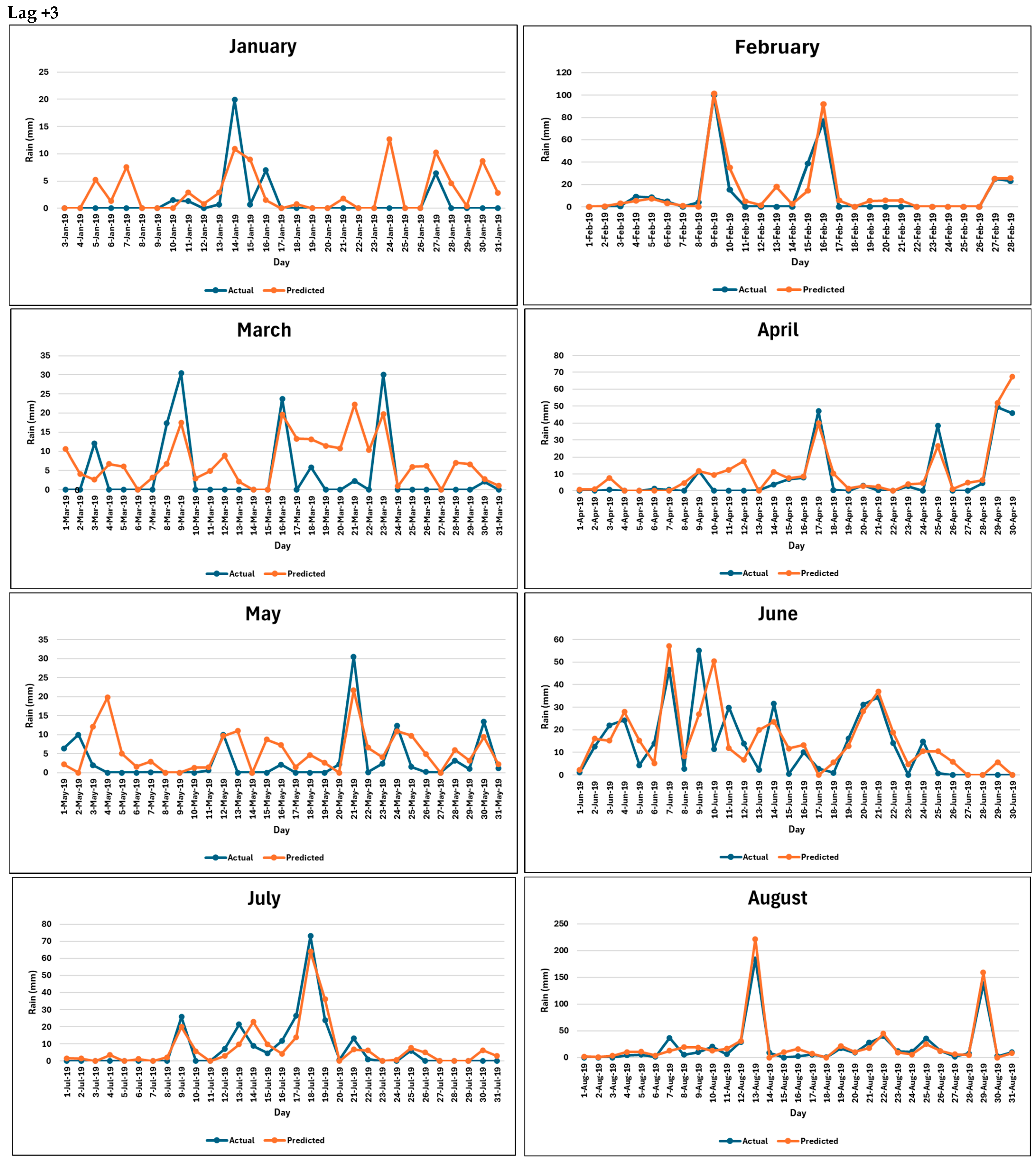
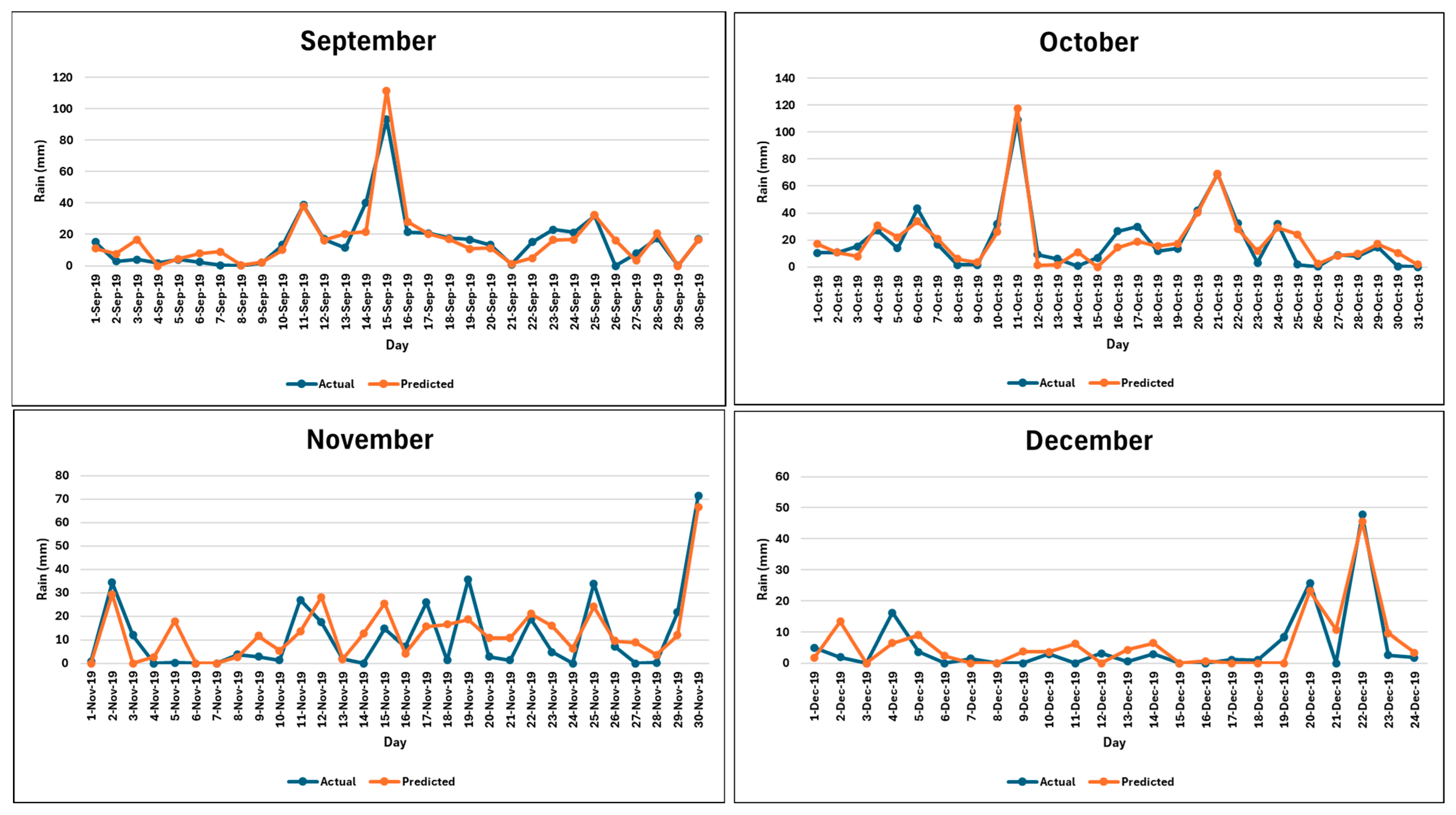
Even though the model was simple and needless to use a High-Performance Computer (HPC), the fitted model could produce better performance in forecasting rainfall values of the target station, especially the extreme values. Figure 3 depicts the fitness of the Bidirectional LSTM model as the rainfall forecasts are closer to the actual rainfall values of the target station for the months of February and August of 2019. The predictions obtained for the rest of the months are illustrated in Figure A2. The two months, February and August, were picked to represent a period from relatively dry and relatively wet seasons of the Ratnapura area. These figures underline that the results obtained from the selected model can be generalized irrespective of the dry or wet season. The major concern of the study is to obtain accurate forecasts for extreme rainfall events. However, the performance of the model in forecasting No or Mild Rainfall, Moderate Rainfall, and Extreme Rainfall events were illustrated for the overall period of the whole year, 2019.
The Meteorology Department of Sri Lanka defined the heavy rainfall cut-off value as 100 mm for Ratnapura. The month of February shows all the rainfall events below 100 mm (no heavy rainfall shows up). The maximum rainfall of that month is recorded as 99.9 mm on 9 February 2019. Figure 3 underscores that the Bidirectional LSTM could closely capture these moderate rainfall patterns in Ratnapura.
On the other hand, the month of August depicts heavy rainfall events on 13 August 2019 (184 mm) and 29 August 2019 (137.4 mm). Figure 3 evidences that these extreme events are accurately forecasted by the model giving 1st day-ahead forecasts of 206.4 mm and 127 mm, respectively. The strong matches between the actual and forecasted rainfall values are the same for the 2nd and 3rd day-ahead forecasting.
Table 6 summarizes the ability of forecasting actual rainfall events, No or Mild Rain (≤12.5 mm), Moderate Rain (>12.5 mm and <100 mm), and Extreme Rain (≥100 mm) by the Bidirectional LSTM model for the testing period 1 January 2019–24 December 2019. The accurately forecasted percentages of each category are also shown in parentheses.
As per Table 6, the accuracy rate of the 1st day-ahead forecast for the first two categories is higher than the 2nd and 3rd day-ahead forecasts. However, the 3rd day-ahead forecasts have well captured the extreme rainfall events. It seems that the 3rd day-ahead forecasts are better than their counterparts in forecasting extreme rainfall. It also seems that the trained Bidirectional LSTM model has the ability identify extreme rainfall even 3 days in advance. However, further experiments are needed to arrive at a conclusion.
By closely examining the plots of actual and predicted rainfall of all 12 months, it was noted that all the No/Mild rainfall cases have predicted correctly or as Moderate rainfall events. Additionally, none of the No/Mild rainfall events are predicted as Extreme rainfall events. During the aforesaid period, only two Mild rainfall events which are closer to 100 mm are predicted as Extreme rainfall events, nevertheless with amounts closer to 100 mm.
These results primarily verified the outperformance of the Bidirectional LSTM model in forecasting rainfall at Ratnapura. The application of the Granger Causality test after Random Forest feature selection was validated by the results obtained through modeling the selected best set of predictors by Random Forest with rainfall at Ratnapura using LSTM methods. The predictions taken for January 2019 depicted the lowest R M S E and M A E values with Autoencoder LSTM. R M S E s are 4.61 (Day + 1), 4.02 (Day + 2), and 4.15 (Day + 3), and M A E s are 3.28 (Day + 1), 3.08 (Day + 2), and 3.32 (Day + 3) which are higher than results obtained with Bidirectional LSTM after applying Granger Causality ( R M S E s are 3.59 (Day + 1), 4.06 (Day + 2), and 4.40 (Day + 3), and M A E s are 2.18 (Day + 1), 2.77 (Day + 2), and 2.71 (Day + 3)).

3.3. Residual Analysis

The study was further continued to examine the adequacy of the fitted Bidirectional LSTM model. In doing so, the randomness of residual series (=Actual rainfall amount − Predicted rainfall amount) was analyzed [81,82] using LJung Box test, Autocorrelation, and Partial-autocorrelation [83,84,85,86,87].
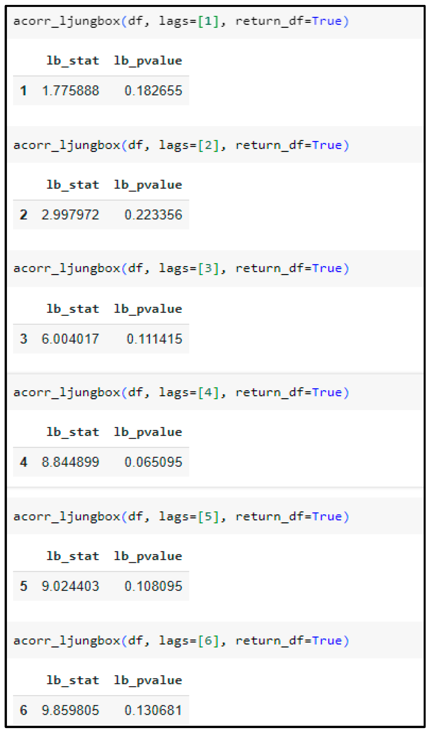
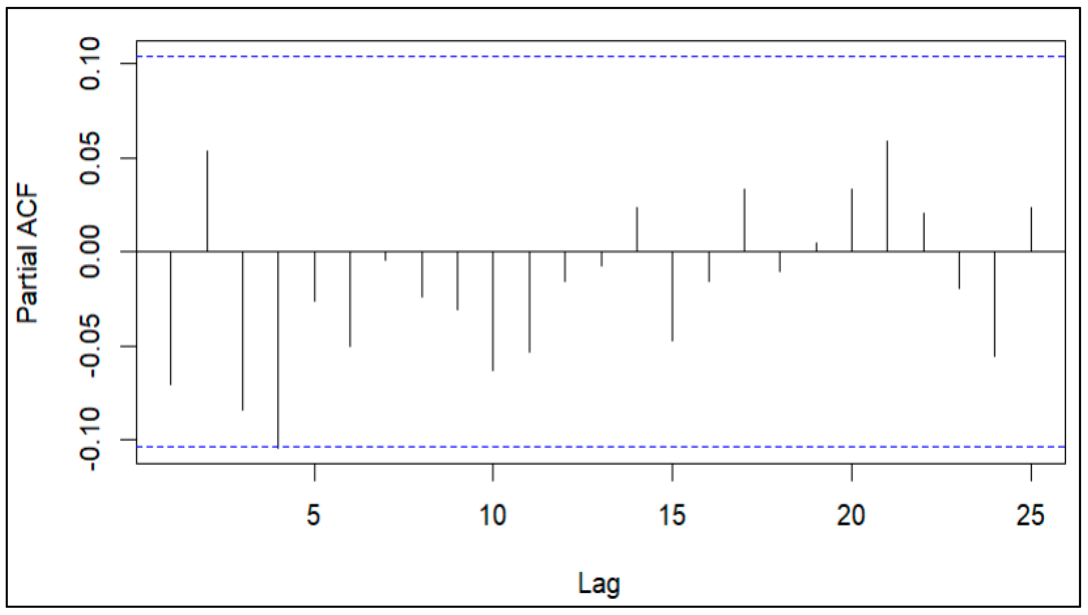
The Ljung Box test verified that the residuals are uncorrelated and follows a White Noise process by not rejecting the Null Hypothesis ( p > 0.05 ), i.e., no significant autocorrelations are found in the residual series. The test results are depicted in Figure A3.
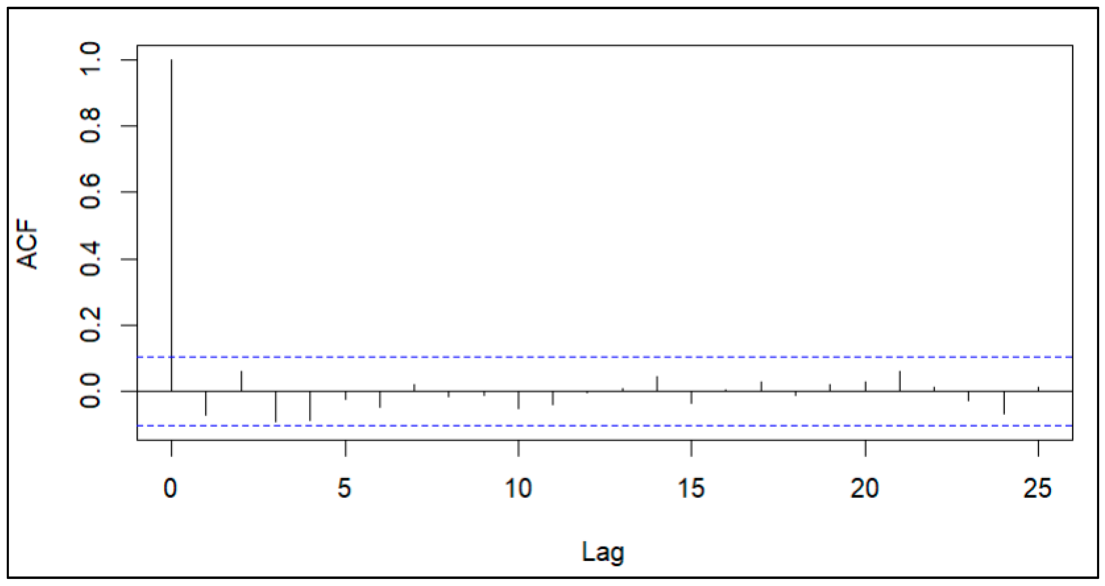
Figure 4 and Figure 5 show the Autocorrelation and Partial-autocorrelation plots of the residual series corresponding to the test period. This plot also evidences that there are no significant autocorrelations among the observations indicating that the residual series is random.
Results of the residual analysis confirm that the fitted Bidirectional LSTM model is adequate for short-term forecasting of the rainfall at Ratnapura station, and it is not required to add any other input variables.

3.4. Verification of Capacity of the Bidirectional LSTM Model in Forecasting Extreme Rainfall Events

The results shown in Section 3.2 confirm that the overall accuracy of the developed forecasting model is inspiring. However, the number of extreme rainfall events included in the testing period is 03 (see Table 5). Even though the forecasting accuracy of the extreme events was considerably high, further studies are needed to verify whether those notable results of the model were given by chance or not. Therefore, a separate period (1 March 2014–31 December 2016) was extracted for training of the same Bidirectional LSTM model with the same optimal features, and it was tested in the period of 1 January 2017–31 December 2017. The selection of the time period was based on the continuous availability of data in the collected data set.
Figure 6 below demonstrates the capability of the Bidirectional LSTM model in forecasting daily rainfall for May and September 2017, which include four extreme events.
The month of May consists of heavy rainfall events on 24 May 2017 (104.1 mm) and 25 May 2017 (348.5 mm). The 1st day-ahead rainfall forecasts for these days are 94.5 mm and 433.4 mm, respectively. The 2nd and 3rd day-ahead forecasts are also close to the actual values. As depicted in Figure 6, the heavy rainfall events in September on 6 September 2017 (135.6 mm) and 07.09.2017 (121.8 mm) were intently captured by the model in all 3 days-ahead forecasting.
Further, Table 7 highlights the number of correctly forecasted extreme rainfall by the Bidirectional LSTM model for the testing period of 1 January 2017–29 December 2017.
Table 7 indicates that the 2nd day-ahead forecasting has correctly captured the four actual extreme events.
Results of Table 5 and Table 6 show that the fitted Bidirectional LSTM model has a high ability (more than 85%) to identify extreme rainfall events 3 days in advance. The selection of appropriate predictor variables may also enhance this ability of forecasting extreme rainfall events.

4. Conclusions

Accurate rainfall modeling is crucial for mitigating future disastrous hazards like flash-flood events. Such a rainfall forecasting model becomes more reliable and applicable if it can capture extremely rare events, called extreme rainfall events, and make accurate forecasts in advance, for example, 3 days-ahead. Moreover, the model should be computationally effective by grabbing the most important predictive features and incorporating their hidden patterns into the model.
Therefore, this study proposes an approach in producing accurate rainfall forecasts using both feature selection methods and deep learning. The optimal set of predictive features were extracted using Random Forest Regression and the Granger Causality test. The selected fourteen features were fed into the Bidirectional LSTM model that was selected as the best through a model comparison. The model training was conducted with the historical moving windows approach and the forecasting horizon was set to 3 days-ahead. The developed model produced very low R M S E (<5 mm) and M A E (<3 mm) values for the test sample comparatively better than the performances depicted in studies, ref. [3] (MAPE > 50%), ref. [7] ( R M S E > 10 mm), ref. [19] ( R M S E > 8 mm and M A E > 4 mm), and [64] ( R M S E > 8 mm).
The study used rainfall and weather data collected from the rainfall gauging station located at Ratnapura in Sri Lanka. The performance of the Bidirectional LSTM, post hoc analysis conducted upon residual series produced by the model, and dual validation of the selected model thoroughly confirmed the suitability of the selected modeling approach in obtaining accurate forecasts, including extreme events for 3 days-ahead rainfall at Ratnapura. This modeling approach may be effectively used to forecast rainfall in other locations around the globe, especially extreme rainfall.
The study is further bridging the research gap existing in the aforesaid climatologically vulnerable area in Sri Lanka. The best forecasting model identified by this study has the ability to forecast the rainfall at Ratnapura with high accuracy.
When conducting the study, the high rate of missing data within a long period of time (30 years of data) was the main problem. Therefore, the time period has to be reduced to 05 years to get a complete and consistent data set for final modeling.
The future study will be directed toward modeling the flood events in the same vulnerable area feeding the rainfall forecasts determined by the identified model.

Author Contributions

Conceptualization, C.T. and S.S.; methodology, S.S., C.T., P.L. and M.M.; software, S.S.; validation, S.S.; formal analysis, S.S.; investigation, C.T., M.M. and P.L.; resources, S.S.; data curation, S.S.; writing—original draft preparation, S.S.; writing—review and editing, C.T. M.M. and P.L.; visualization, S.S.; supervision, C.T., P.L. and M.M.; project administration, C.T.; funding acquisition, C.T. All authors have read and agreed to the published version of the manuscript.

Funding

This research was funded by the Research Grant of the University of Colombo, Sri Lanka, grant number AP/3/2019/CG/30.

Data Availability Statement

The data that support the findings of this study are available from the authors upon reasonable request.

Acknowledgments

The authors wish to acknowledge the University of Colombo, Sri Lanka, for the monetary support.

Conflicts of Interest

The authors declare no conflicts of interest.

Appendix A

Table A1. Random Forest Regression—feature importance.
XScoreRankXScoreRankXScoreRank
arain-10.0643821Tmax-20.01443525WsM-20.00873349
krig-10.0558082RhN-10.01396226ClM-20.0081950
MslpM-30.0422583WdM-10.01381327SOI-30.00751451
DwE-20.0339794DwE-30.01376828SOI-20.00735152
krig-30.0337915MslpE-20.01319629WdM-20.00702153
Evp-30.031496arain-20.01300130ClM-10.00693254
DwM-10.0303267Evp-20.01284531Con_rainD-10.00664455
SunS-30.0260238Tmax-10.01252732SOI-10.00651656
Evp-10.0244429Tmin-10.01243333Con_rainD-30.006257
MslpE-10.02375610RhN-20.01234834ClE-20.00540658
RhD-10.02263111WsE-10.01195235ClE-30.00538459
Tmin-30.02128612arain-30.01147336Con_rainD-20.00499160
MslpE-30.02109713RhD-20.01136337ClE-10.00407161
krig-20.01966414WdE-20.01110538satellite-30.00389862
SunS-10.01950315DwM-20.01097839Con_dryD-20.00357363
DwM-30.01809316WsM-10.0107640Con_dryD-30.0023364
MslpM-10.01739617rain-10.0106941nino-20.00152765
WsE-20.01695618WsE-30.01048842satellite-10.00149966
DwE-10.01628519WdE-30.01002643nino-10.00137367
Tmax-30.01626320RhN-30.01001944nino-30.00128568
SunS-20.01594821WdE-10.00994445satellite-20.00125969
RhD-30.01559422WdM-30.00984146Con_dryD-10.00111670
WsM-30.01463323Tmin-20.00972547rain-30.00083971
MslpM-20.01451124ClM-30.00875448rain-20.00078772
Table A2. Random Forest Regression models obtained through backward elimination.
TrainingTesting
Number of FeaturesR2RMSEMAER2RMSEMAE
1−0.179521.100311.7105−0.121916.025010.24466
2−0.0376119.832011.1934−0.0772515.702910.3040
30.02150519.301411.3090−0.0274115.335310.4247
40.00595719.504711.36200.03287314.878610.2054
5−0.0026819.481511.35430.08001814.511410.0594
60.01327819.355011.28620.04241314.805110.4354
70.00920719.352411.26420.0259614.931710.3643
80.00196219.391211.35690.05167914.733210.2129
9−0.008419.497211.47260.024714.941110.4089
10−0.007319.422211.41700.012915.031210.4358
110.015819.315711.37960.005615.086710.4711
120.010119.312111.4324−0.004015.159410.4680
130.009219.316111.4465−0.013615.231910.5142
140.004919.363211.4963−0.004615.163810.5279
150.012019.323111.4601−0.029115.348110.5831
16−0.000219.379711.4916−0.032115.370510.5693
17−0.004919.431611.5121−0.040615.433410.6077
18−0.007919.467911.5468−0.043615.455810.6201
19−0.010519.473311.5540−0.038315.416110.6424
20−0.012319.517011.6042−0.031715.367210.6127
21−0.008419.515611.5922−0.028015.340010.6164
22−0.005619.480511.5965−0.033515.380910.6181
230.000119.466111.5491−0.029815.353510.5880
24−0.010519.485311.5909−0.026315.326710.5838
25−0.012619.497011.5897−0.017615.261710.5336
26−0.010219.497311.5775−0.015615.247210.5101
27−0.004919.447711.5785−0.022915.301510.5633
28−0.006919.492211.5962−0.020015.280210.5384
29−0.008719.470711.6265−0.026815.330810.5958
30−0.005519.467511.6042−0.008915.196510.5306
31−0.007919.487411.6298−0.022315.297010.5888
32−0.009419.491611.6369−0.024715.315310.5707
33−0.011519.519611.6441−0.035815.397510.6290
34−0.012519.507811.6534−0.030615.358910.6261
35−0.012319.541711.6789−0.037515.410610.67682
36−0.016319.566611.6731−0.035015.391910.6520
37−0.015019.549411.6880−0.034815.390710.6676
38−0.016519.574811.7174−0.039415.424410.7113
39−0.016519.588311.7245−0.035815.397610.7152
40−0.022719.584311.7440−0.027515.335610.6883
41−0.020119.602011.7252−0.033615.381410.6883
42−0.024119.601911.7253−0.032915.376110.6903
43−0.018719.606711.7185−0.033315.379410.7274
44−0.017519.592211.7277−0.036115.399810.7273
45−0.020519.595111.7326−0.035615.396710.7319
46−0.021019.607011.7214−0.031615.366810.7050
47−0.020919.593011.7347−0.035615.396410.7023
480.018719.587411.7058−0.030415.358010.6828
49−0.019519.583611.7230−0.028215.341110.6673
50−0.020619.598511.7161−0.026615.329410.6545
51−0.023819.584011.7407−0.040015.429310.7135
52−0.023719.609411.7457−0.037515.410710.7151
53−0.021319.619211.7448−0.021415.290310.6330
54−0.023119.621111.7492−0.028615.344310.6539
55−0.019019.604411.7468−0.028415.342710.6515
56−0.016919.613611.7476−0.027015.332610.6323
57−0.023519.604511.7517−0.032315.371510.6643
58−0.023619.602211.7543−0.027115.332910.6479
59−0.022819.600511.7327−0.030615.359510.6586
60−0.022619.598311.7545−0.030115.355710.6597
61−0.021919.598311.7519−0.023015.302210.6315
62−0.021819.604111.7305−0.029815.353010.6674
63−0.018919.589511.7310−0.028115.340810.6527
64−0.024319.627411.7374−0.023915.308910.6453
65−0.021819.620411.7403−0.025815.323410.6613
66−0.022019.603511.7437−0.028515.343110.6806
67−0.020419.597511.7346−0.026215.326110.6556
68−0.023419.606011.7363−0.026015.324610.6438
69−0.023319.610411.7214−0.026315.327410.6439
70−0.020619.617611.7527−0.027315.334210.6593
71−0.022719.630511.7416−0.027515.336210.6570
72−0.021919.604011.7263−0.029015.347410.6818

Appendix B

Figure A1. The training loss vs. validation loss of the Bidirectional LSTM model for January, May, August, and November in 2019.
Forecasting 06 00056 g0a1
Figure A2. The monthly rainfall forecasts by the Bidirectional LSTM model.
Forecasting 06 00056 g0a2aForecasting 06 00056 g0a2bForecasting 06 00056 g0a2cForecasting 06 00056 g0a2dForecasting 06 00056 g0a2e
Figure A3. Ljung Box test results for selected lags of residual series.
Forecasting 06 00056 g0a3

References

  1. Nagahamulla, H.R.K.; Ratnayake, U.R.; Ratnaweera, A. Monsoon rainfall forecasting in Sri Lanka using artificial neural networks. In Proceedings of the 2011 6th International Conference on Industrial and Information Systems, Kandy, Sri Lanka, 16–19 August 2011; pp. 305–309. [Google Scholar] [CrossRef]
  2. Perera, H.; Sonnadara, D.; Jayewardene, D. Forecasting the Occurrence of Rainfall in Selected Weather Stations in the Wet and Dry Zones of Sri Lanka. Sri Lankan J. Phys. 2002, 3, 39–52. [Google Scholar] [CrossRef]
  3. Haq, D.Z.; Novitasari, D.C.R.; Hamid, A.; Ulinnuha, N.; Arnita; Farida, Y.; Nugraheni, R.D.; Nariswari, R.; Ilham; Rohayani, H.; et al. Long Short-Term Memory Algorithm for Rainfall Prediction Based on El-Nino and IOD Data. Procedia Comput. Sci. 2021, 179, 829–837. [Google Scholar] [CrossRef]
  4. Kundu, S.; Biswas, S.K.; Tripathi, D.; Karmakar, R.; Majumdar, S.; Mandal, S. A Review on Rainfall Forecasting using Ensemble Learning Techniques. e-Prim. Adv. Electr. Eng. Electron. Energy 2023, 6, 100296. [Google Scholar] [CrossRef]
  5. Chang, C.B. A case study of excessive rainfall forecasting. Meteorol. Atmos. Phys. 1998, 66, 215–227. [Google Scholar] [CrossRef]
  6. Ridwan, W.M.; Sapitang, M.; Aziz, A.; Kushiar, K.F.; Ahmed, A.N.; El-Shafie, A. Rainfall forecasting model using machine learning methods: Case study Terengganu, Malaysia. Ain Shams Eng. J. 2020, 12, 1651–1663. [Google Scholar] [CrossRef]
  7. Yang, B.; Chen, L.; Singh, V.P.; Yi, B.; Leng, Z.; Zheng, J.; Song, Q. A Method for Monthly Extreme Precipitation Forecasting with Physical Explanations. Water 2023, 15, 1545. [Google Scholar] [CrossRef]
  8. Singhal, A.; Raman, A.; Jha, S.K. Potential Use of Extreme Rainfall Forecast and Socio-Economic Data for Impact-Based Forecasting at the District Level in Northern India. Front. Earth Sci. 2022, 10, 846113. [Google Scholar] [CrossRef]
  9. Saubhagya, S.; Tilakaratne, C.; Mammadov, M.; Lakraj, P. An Application of Ensemble Spatiotemporal Data Mining Techniques for Rainfall Forecasting. Eng. Proc. 2023, 39, 6. [Google Scholar] [CrossRef]
  10. Hong, W.C. Rainfall forecasting by technological machine learning models. Appl. Math. Comput. 2008, 200, 41–57. [Google Scholar] [CrossRef]
  11. Hand, W.H.; Fox, N.I.; Collier, C.G. A study of twentieth—Century extreme rainfall events in the United Kingdom with implications for forecasting. Meteorol. Appl. 2004, 11, 15–31. [Google Scholar] [CrossRef]
  12. Sangiorgio, M.; Barindelli, S.; Biondi, R.; Solazzo, E.; Realini, E.; Venuti, G.; Guariso, G. Improved Extreme Rainfall Events Forecasting Using Neural Networks and Water Vapor Measures. In Proceedings of the ITISE 2019 (6th International Conference on Time Series and Forecasting), Granada, Spain, 25–27 September 2019. [Google Scholar]
  13. Araújo, A.d.S.; Silva, A.R.; Zárate, L.E. Extreme Precipitation Prediction Based on Neural Network Model—A Case Study for Southeastern Brazil. J. Hydrol. 2022, 606, 127454. [Google Scholar] [CrossRef]
  14. Gouda, K.; Nahak, S.; Goswami, P. Evaluation of a GCM in seasonal forecasting of extreme rainfall events over continental India. Weather Clim. Extrem. 2018, 21, 10–16. [Google Scholar] [CrossRef]
  15. Samantray, P.; Gouda, K.C. A review on the extreme rainfall studies in India. Nat. Hazards Res. 2023, 4, 347–356. [Google Scholar] [CrossRef]
  16. Luk, K.C.; Ball, J.E.; Sharma, A. An application of artificial neural networks for rainfall forecasting. Math. Comput. Model. 2001, 33, 683–693. [Google Scholar] [CrossRef]
  17. Rathnayake, V.; Premaratne, H.; Sonnadara, D. Performance of neural networks in forecasting short range occurrence of rainfall. J. Natl. Sci. Found. Sri Lanka 2011, 39, 251–260. [Google Scholar] [CrossRef]
  18. Ni, L.; Wang, D.; Singh, V.P.; Wu, J.; Wang, Y.; Tao, Y.; Zhang, J. Streamflow and rainfall forecasting by two long short-term memory-based models. J. Hydrol. 2020, 583, 124296. [Google Scholar] [CrossRef]
  19. Nagahamulla, H.R.K.; Ratnayake, U.R.; Ratnaweera, A. Artificial neural network ensembles in time series forecasting: An application of rainfall forecasting in Sri Lanka. Int. J. Adv. ICT Emerg. Reg. (ICTer) 2014, 6, 1–11. [Google Scholar] [CrossRef]
  20. Bushara, N.; Abraham, A. Novel ensemble method for long term rainfall prediction. Int. J. Comput. Inf. Syst. Ind. Manag. Appl. 2015, 7, 116–130. [Google Scholar]
  21. Mohd, R.; Butt, M.A.; Baba, M.Z. Comparative study of rainfall prediction modeling techniques (A case study on Srinagar, J&K, India). Asian J. Comput. Sci. Technol. 2018, 7, 13–19. [Google Scholar]
  22. Anwar, M.T.; Winarno, E.; Hadikurniawati, W.; Novita, M. Rainfall prediction using extreme gradient boosting. J. Phys. Conf. Ser. 2021, 1869, 012078. [Google Scholar] [CrossRef]
  23. Liyew, C.M.; Melese, H.A. Machine learning techniques to predict daily rainfall amount. J. Big Data 2021, 8, 1–11. [Google Scholar] [CrossRef]
  24. Chowdhary, M.; Anabarasi, M. Enhanced rainfall predictions using stacking technique. Int. J. Emerg. Technol. Innov. Res. 2020, 7, 750–755. [Google Scholar]
  25. Singh, G.; Kumar, D. Hybrid prediction models for rainfall forecasting. In Proceedings of the 9th International Conference on Cloud Computing, Data Science & Engineering (Confluence), Noida, India, 10–11 January 2019; IEEE: New York, NY, USA, 2019; pp. 392–396. [Google Scholar]
  26. Osman, A.I.A.; Ahmed, A.N.; Chow, M.F.; Huang, Y.F.; El-Shafie, A. Extreme gradient boosting (Xgboost) model to predict the groundwater levels in Selangor Malaysia. Ain Shams Eng. J. 2021, 12, 1545–1556. [Google Scholar] [CrossRef]
  27. Wanless, A.C.; Riley, R.E. Examining Extreme Rainfall Forecast and Communication Processes in the South-Central United States. Weather Clim. Soc. 2023, 15, 787–800. [Google Scholar] [CrossRef]
  28. Gope, S.; Sarkar, S.; Mitra, P.; Ghosh, S. Early Prediction of Extreme Rainfall Events: A Deep Learning Approach. In Advances in Data Mining. Applications and Theoretical Aspects; Springer: Cham, Switzerland, 2016; Volume 9728, pp. 154–167. [Google Scholar] [CrossRef]
  29. Kursa, M.B.; Rudnicki, W.R. The All Relevant Feature Selection using Random Forest. arXiv 2011, arXiv:1106.5112. [Google Scholar]
  30. Pudjihartono, N.; Fadason, T.; Kempa-Liehr, A.W.; O’Sullivan, J.M. A Review of Feature Selection Methods for Machine Learning-Based Disease Risk Prediction. Front. Bioinform. 2022, 2, 927312. [Google Scholar] [CrossRef]
  31. Brownlee, J. How to Choose a Feature Selection Method For Machine Learning. 2020. Available online: https://machinelearningmastery.com/feature-selection-with-real-and-categorical-data/ (accessed on 1 June 2024).
  32. Nguyen, C.; Wang, Y.; Nguyen, H.N. Random forest classifier combined with feature selection for breast cancer diagnosis and prognostic. J. Biomed. Sci. Eng. 2013, 6, 551–560. [Google Scholar] [CrossRef]
  33. Niu, D.; Wang, K.; Sun, L.; Wu, J.; Xu, X. Short-term photovoltaic power generation forecasting based on random forest feature selection and CEEMD: A case study. Appl. Soft Comput. 2020, 93, 106389. [Google Scholar] [CrossRef]
  34. Niu, D.; Wang, K.; Sun, L.; Wu, J.; Xu, X. LSTM integrated with Boruta-random forest optimiser for soil moisture estimation under RCP4.5 and RCP8.5 global warming scenarios. Stoch. Environ. Res. Risk Assess. 2021, 35, 1851–1881. [Google Scholar] [CrossRef]
  35. Li, X.; Chen, W.; Zhang, Q.; Wu, L. Building Auto-Encoder Intrusion Detection System Based on Random Forest Feature Selection. Comput. Secur. 2020, 95, 101851. [Google Scholar] [CrossRef]
  36. Sylvester, E.V.A.; Bentzen, P.; Bradbury, I.R.; Clément, M.; Pearce, J.; Horne, J.; Beiko, R.G. Applications of random forest feature selection for fine-scale genetic population assignment. Evol. Appl. 2017, 11, 153–165. [Google Scholar] [CrossRef] [PubMed]
  37. Liu, Y.; Mu, Y.; Chen, K.; Li, Y.; Guo, J. Daily Activity Feature Selection in Smart Homes Based on Pearson Correlation Coefficient. Neural Process. Lett. 2020, 51, 1771–1787. [Google Scholar] [CrossRef]
  38. Nasir, I.M.; Khan, M.A.; Yasmin, M.; Shah, J.H.; Gabryel, M.; Scherer, R.; Damaševičius, R. Pearson Correlation-Based Feature Selection for Document Classification Using Balanced Training. Sensors 2020, 20, 6793. [Google Scholar] [CrossRef]
  39. Saidi, R.; Bouaguel, W.; Essoussi, N. Hybrid Feature Selection Method Based on the Genetic Algorithm and Pearson Correlation Coefficient. In Machine Learning Paradigms: Theory and Application; Springer: Cham, Switzerland, 2019. [Google Scholar] [CrossRef]
  40. Chen, P.; Li, F.; Wu, C. Research on Intrusion Detection Method Based on Pearson Correlation Coefficient Feature Selection Algorithm. J. Phys. Conf. Ser. 2021, 1757, 012054. [Google Scholar] [CrossRef]
  41. Risqiwati, D.; Wibawa, A.D.; Pane, E.S.; Islamiyah, W.R.; Tyas, A.E.; Purnomo, M.H. Feature Selection for EEG-Based Fatigue Analysis Using Pearson Correlation. In Proceedings of the 2020 International Seminar on Intelligent Technology and Its Applications (ISITIA), Surabaya, Indonesia, 22–23 July 2020; pp. 164–169. [Google Scholar] [CrossRef]
  42. Saikhu, A.; Nopember, I.T.S.; Arifin, A.; Fatichah, C. Correlation and Symmetrical Uncertainty-Based Feature Selection for Multivariate Time Series Classification. Int. J. Intell. Eng. Syst. 2019, 12, 129–137. [Google Scholar] [CrossRef]
  43. Attanasio, A.; Pasini, A.; Triacca, U. Granger Causality Analyses for Climatic Attribution. Atmos. Clim. Sci. 2013, 3, 515–522. [Google Scholar] [CrossRef]
  44. Li, H.; Li, M. Modeling of Precipitation Prediction Based on Causal Analysis and Machine Learning. Atmosphere 2023, 14, 1396. [Google Scholar] [CrossRef]
  45. McGraw, M.C.; Barnes, E.A. Memory Matters: A Case for Granger Causality in Climate Variability Studies. J. Clim. 2018, 31, 3289–3300. [Google Scholar] [CrossRef]
  46. He, Y.; Lee, E. Empirical Relationships of Sea Surface Temperature and Vegetation Activity with Summer Rainfall Variability over the Sahel. Earth Interact. 2015, 20, 1–18. [Google Scholar] [CrossRef]
  47. Silva, F.N.; Vega-Oliveros, D.A.; Yan, X.; Flammini, A.; Menczer, F.; Radicchi, F.; Kravitz, B.; Fortunato, S. Detecting climate teleconnections with Granger causality. Geophys. Res. Lett. 2020, 48, e2021GL094707. [Google Scholar] [CrossRef]
  48. Xu, F.; Sun, S.; Zhao, P.; Jia, S. Granger causal weather time series forecasting simulation combined with mutual information. J. Phys. Conf. Ser. 2021, 1861, 012061. [Google Scholar] [CrossRef]
  49. Greeshma, K.; Pramod, N.; Nair, M.S. Deep Learning Approach to Rainfall Prediction. Master’s Thesis, Amrita School of Physical Sciences, Coimbatore, India, 2023. [Google Scholar] [CrossRef]
  50. Amir, G.; Sanandaji, B.M.; Ghaderi, F. Deep forecast: Deep learning-based spatio-temporal forecasting. arXiv 2017, arXiv:1707.08110. [Google Scholar]
  51. Wang, H.; Lei, Z.; Zhang, X.; Zhou, B.; Peng, J. A review of deep learning for renewable energy forecasting. Energy Convers. Manag. 2019, 198, 111799. [Google Scholar] [CrossRef]
  52. Lim, B.; Zohren, S. Time-series forecasting with deep learning: A survey. Philos. Trans. R. Soc. A 2021, 379, 20200209. [Google Scholar] [CrossRef]
  53. Basha, C.Z.; Bhavana, N.; Bhavya, P.; Sowmya, V. Rainfall prediction using machine learning & deep learning techniques. In Proceedings of the 2020 International Conference on Electronics and Sustainable Communication Systems (ICESC), Coimbatore, India, 2–4 July 2020; IEEE: New York, NY, USA; pp. 92–97. [Google Scholar]
  54. Yen, M.H.; Liu, D.W.; Hsin, Y.C.; Lin, C.E.; Chen, C.C. Application of the deep learning for the prediction of rainfall in Southern Taiwan. Sci. Rep. 2019, 9, 12774. [Google Scholar] [CrossRef]
  55. Hernández, E.; Sanchez-Anguix, V.; Julian, V.; Palanca, J.; Duque, N. Rainfall prediction: A deep learning approach. In Hybrid Artificial Intelligent Systems, Proceedings of the 11th International Conference, HAIS 2016, Seville, Spain, 18–20 April 2016, Proceedings 11; Springer International Publishing: Cham, Switzerland, 2016; pp. 151–162. [Google Scholar]
  56. Narejo, S.; Jawaid, M.M.; Talpur, S.; Baloch, R.; Pasero, E.G.A. Multi-step rainfall forecasting using deep learning approach. PeerJ Comput. Sci. 2021, 7, e514. [Google Scholar] [CrossRef]
  57. Barrera-Animas, A.Y.; Oyedele, L.O.; Bilal, M.; Akinosho, T.D.; Delgado, J.M.D.; Akanbi, L.A. Rainfall prediction: A comparative analysis of modern machine learning algorithms for time-series forecasting. Mach. Learn. Appl. 2022, 7, 100204. [Google Scholar] [CrossRef]
  58. Xiang, Z.; Yan, J.; Demir, I. A rainfall-runoff model with LSTM based sequence to sequence learning. Water Resour. Res. 2020, 56, e2019WR025326. [Google Scholar] [CrossRef]
  59. Hou, G.H.; Li, J.N.; Huang, X.S.; Ban, J.R.; Wang, Y.B.; Zhou, Y. Research on rainfall prediction based on LSTM, RF and SVM models. In Proceedings of the 2nd International Conference on Computer Vision, Image, and Deep Learning, Liuzhou, China, 25–27 June 2021; SPIE: Bellingham, WA, USA, 2021; Volume 11911, pp. 225–231. [Google Scholar]
  60. Aderyani, F.R.; Mousavi, S.J.; Jafari, F. Short-term rainfall forecasting using machine learning-based approaches of PSO-SVR, LSTM and CNN. J. Hydrol. 2022, 614, 128463. [Google Scholar] [CrossRef]
  61. Poornima, S.; Pushpalatha, M. Prediction of rainfall using intensified LSTM based recurrent neural network with weighted linear units. Atmosphere 2019, 10, 668. [Google Scholar] [CrossRef]
  62. Ponnoprat, D. Short-term daily precipitation forecasting with seasonally-integrated autoencoder. Appl. Soft Comput. 2021, 102, 107083. [Google Scholar] [CrossRef]
  63. Gu, N.; Wan, D. Trend analysis of extreme rainfall based on BP neural network. In Proceedings of the 2010 Sixth International Conference on Natural Computation, Yantai, China, 10–12 August 2010; Volume 4, pp. 1925–1928. [Google Scholar] [CrossRef]
  64. Perera, V.A.P.C.; Peiris, K.G.H.S. An Improved Statistical Method for Rainfall Forecasting in Sri Lanka using the WRF Model. In Proceedings of the 2020 International Conference and Utility Exhibition on Energy, Environment and Climate Change (ICUE), Pattaya, Thailand, 20–22 October 2020; IEEE: New York, NY, USA, 2020; pp. 1–7. [Google Scholar]
  65. Saparamadu, S.; Bandara, S.; Hewawasam, C.; Abeysinghe, U. Mathematical Models to Forecast Rainfall for Disaster Conditions in Sri Lanka. EPH-Int. J. Math. Stat. 2018, 4, 16–22. [Google Scholar] [CrossRef]
  66. Punyawardena, B.; Cherry, N.J. Assessment of the predictability of the seasonal rainfall in Ratnapura using Southern Oscillation and its two extremes. J. Natl. Sci. Found. Sri Lanka 1999, 27, 187–195. [Google Scholar] [CrossRef]
  67. Hemachandra, E.M.G.P.; Dayawansa, N.D.K.; De Silva, R. Developing a Composite Map of Vulnerability to Rainfall Extremes in Sri Lanka. In Water, Flood Management and Water Security Under a Changing Climate; Springer: Cham, Switzerland, 2020. [Google Scholar] [CrossRef]
  68. Darji, M.P.; Dabhi, V.K.; Prajapati, H.B. Rainfall forecasting using neural network: A survey. In Proceedings of the 2015 International Conference on Advances in Computer Engineering and Applications, Ghaziabad, India, 19–20 March 2015. [Google Scholar] [CrossRef]
  69. Ratnayake, U.; Sachindra, D.; Nandalal, K.D.W. Rainfall forecasting for flood prediction in the Nilwala Basin. In Proceedings of the International Conference on Sustainable Built Environments 2010, Kandy, Sri Lanka, 13–14 December 2010. [Google Scholar]
  70. Fawagreh, K.; Gaber, M.M.; Elyan, E. Random Forests: From Early Developments to Recent Advancements. Syst. Sci. Control. Eng. 2014, 2, 602–609. [Google Scholar] [CrossRef]
  71. Goehry, B.; Yan, H.; Goude, Y.; Massart, P.; Poggi, J.-M. Random Forests for Time Series. REVSTAT-Stat. J. 2023, 21, 283–302. [Google Scholar]
  72. Liaw, A.; Wiener, M. Classification and Regression by Random Forest. Forest 2001, 23, 19–22. [Google Scholar]
  73. Granger, C.W.J. Investigating Causal Relations by Econometric Models and Cross-Spectral Methods. In Essays in Econometrics: Collected Papers of Clive W. J. Granger; Ghysels, E., Swanson, N.R., Watson, M.W., Eds.; Econometric Society Monographs; Cambridge University Press: Cambridge, UK, 2001; pp. 31–47. [Google Scholar]
  74. Understanding LSTM Networks. Available online: https://colah.github.io/posts/2015-08-Understanding-LSTMs/ (accessed on 13 July 2024).
  75. Brownlee, J. Stacked Long Short-Term Memory Networks. 2019. Available online: https://machinelearningmastery.com/stacked-long-short-term-memory-networks/ (accessed on 10 June 2024).
  76. Sahar, A.; Han, D. An LSTM-based Indoor Positioning Method Using Wi-Fi Signals. In Proceedings of the ICVISP 2018: The 2nd International Conference on Vision, Image and Signal Processing, Las Vegas, NV, USA, 27–29 August 2018; pp. 1–5. [Google Scholar] [CrossRef]
  77. Brownlee, J. How to Develop LSTM Models for Time Series Forecasting. 2020. Available online: https://machinelearningmastery.com/how-to-develop-lstm-models-for-time-series-forecasting/ (accessed on 10 June 2024).
  78. Saubhagya, S.; Tilakaratne, C.; Lakraj, P.; Mammadov, M. A Novel Hybrid Spatiotemporal Missing Value Imputation Approach for Rainfall Data: An Application to the Ratnapura Area, Sri Lanka. Appl. Sci. 2024, 14, 999. [Google Scholar] [CrossRef]
  79. Fan, H.; Wu, S.; Chen, N.; Gao, B.; Xu, Y. A New Approach for Short-term Time Series Forecasting. IOP Conf. Ser. Mater. Sci. Eng. 2019, 646, 012015. [Google Scholar] [CrossRef]
  80. Hyndman, R.J.; Athanasopoulos, G. Forecasting: Principles and Practice, 2nd ed.; 2018; Available online: https://otexts.com/fpp2/long-short-ts.html (accessed on 10 June 2024).
  81. Xu, D.-M.; Hu, X.-X.; Wang, W.-C.; Chau, K.-W.; Zang, H.-F.; Wang, J. A new hybrid model for monthly runoff prediction using ELMAN neural network based on decomposition-integration structure with local error correction method. Expert Syst. Appl. 2023, 238, 121719. [Google Scholar] [CrossRef]
  82. Broersen, P.M.T. Error Correction of Rainfall-Runoff Models With the ARMAsel Program. IEEE Trans. Instrum. Meas. 2007, 56, 2212–2219. [Google Scholar] [CrossRef]
  83. Mondal, P.; Shit, L.; Goswami, S. Study of Effectiveness of Time Series Modeling (Arima) in Forecasting Stock Prices. Int. J. Comput. Sci. Eng. Appl. 2014, 4, 13–29. [Google Scholar] [CrossRef]
  84. Moffat, I.U.; Akpan, E.A. White Noise Analysis: A Measure of Time Series Model Adequacy. Appl. Math. 2019, 10, 989–1003. [Google Scholar] [CrossRef]
  85. Hassani, H.; Yeganegi, M.R. Selecting optimal lag order in Ljung–Box test. Phys. A Stat. Mech. Appl. 2019, 541, 123700. [Google Scholar] [CrossRef]
  86. Lee, T. Wild bootstrap Ljung–Box test for cross correlations of multivariate time series. Econ. Lett. 2016, 147, 59–62. [Google Scholar] [CrossRef]
  87. How to Perform a Ljung-Box Test in Python. 2021. Available online: https://koalatea.io/python-ljung-box-test/ (accessed on 10 June 2024).
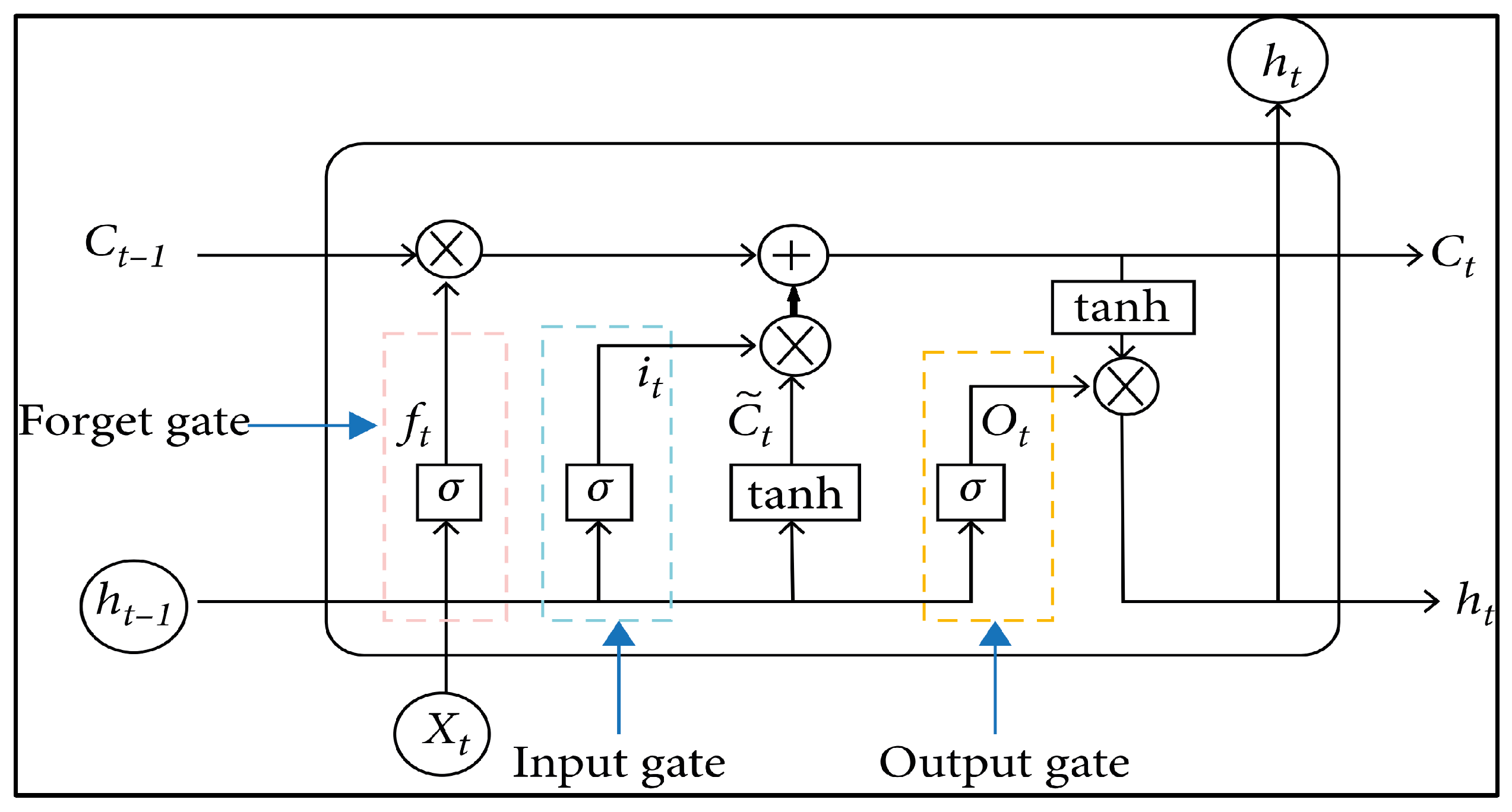
Figure 1. LSTM structure diagram (adapted with permission from Ref. [9]).
Forecasting 06 00056 g001
Figure 2. Training input and testing output structure of LSTM Bidirectional model.
Forecasting 06 00056 g002
Figure 3. The 1st to 3rd day-ahead forecasts of rainfall at Ratnapura for February and August in 2019.
Forecasting 06 00056 g003
Figure 4. The Autocorrelation function for residual series (The horizontal dashed lines or bands indicate the 95% confidence interval).
Forecasting 06 00056 g004
Figure 5. The Partial autocorrelation function for residual series (The horizontal dashed lines or bands indicate the 95% confidence interval).
Forecasting 06 00056 g005
Figure 6. The 3 days-ahead forecasts of rainfall at Ratnapura for May and September in 2017.
Forecasting 06 00056 g006
Table 1. Optimal parameter settings in Random Forest Regression model.
ParametersValue
n_estimator 100
n_samples60%
max_featuresn_features
k (in k-fold cross-validation)5
Table 2. Causal predictor variables and significant lags.
Predictor VariableSignificant Past Lag Range (at 5% Significance Level)Minimum of p Values Within 14 Lags
accumulated rain1–20.0007
kriging interpolation1–90.0009
dew point (evening)more than 14<1 × 10⁻¹²
evaporationmore than 140.0001
dew point (morning)more than 14<1 × 10⁻¹²
sunshine hoursmore than 14<1 × 10⁻¹²
relative humidity (day)more than 14<1 × 10⁻¹²
temperature (minimum)1–50.0001
relative humidity (night)more than 14<1 × 10⁻¹²
temperature (maximum)1–20.0055
cloud amount (morning)10.0127
cloud amount (evening)more than 14<1 × 10⁻¹²
continuous dry days1–12<1 × 10⁻¹²
continuous wet days1–20.0014
Table 3. Performance of Stacked LSTM, Bidirectional LSTM and Encoder-Decoder LSTM.
Model Stacked LSTMBidirectional LSTMEncoder-Decoder LSTM
Forecasted Day-Ahead123123123
JanuaryRMSE4.344.814.943.594.064.404.024.575.49
MAE3.433.692.972.182.772.712.993.263.57
MayRMSE11.1010.109.994.835.405.978.077.137.47
MAE8.147.708.122.853.764.096.685.665.92
AugustRMSE26.8020.6042.009.5010.6011.2030.7028.9038.10
MAE16.7014.5023.706.387.607.8518.0016.5019.10
NovemberRMSE16.2015.9018.507.289.869.2415.7016.1016.70
MAE11.9011.6014.005.197.067.6912.6011.5012.10
The lowest R M S E s and M A E s values are depicted in bold.
Table 4. Comparison of the rainfall class-wise prediction capability of Stacked LSTM, Bidirectional LSTM, and Encoder-Decoder LSTM models for selected months in 2019.
Rainfall Event/ClassNumber of Days Forecasted Ahead
123
Stacked LSTMActual Count Accurately Forecasted Count Actual Count Accurately Forecasted Count Actual Count Accurately Forecasted Count
No/Mild Rain3030 (100)29 29 (100)2828 (100)
JanuaryModerate Rain10 (0)10 (0)10 (0)
Extreme Rain000000
No/Mild Rain2922 (76)2824 (86)2723 (85)
MayModerate Rain20 (0)20 (0)20 (0)
Extreme Rain000000
No/Mild Rain2212 (55)2110 (48)209 (45)
AugustModerate Rain74 (57)74 (57)74 (57)
Extreme Rain21 (50)21 (50)20 (0)
No/Mild Rain2010 (50)199 (47)1910 (53)
NovemberModerate Rain108 (80)108 (80)94 (44)
Extreme Rain000000
Bidirectional LSTM
No/Mild Rain3030 (100)2929 (100)2827 (96)
JanuaryModerate Rain10 (0)10 (0)10 (0)
Extreme Rain000000
No/Mild Rain2927 (93)2825 (89)2726 (96)
MayModerate Rain21 (50)21 (50)21 (50)
Extreme Rain000000
No/Mild Rain2217 (77)2112 (57)2016 (80)
AugustModerate Rain77 (100)75 (71)76 (86)
Extreme Rain22 (100)22 (100)22 (100)
No/Mild Rain2018 (90)1914 (74)1915 (79)
NovemberModerate Rain109 (90)108 (80)98 (89)
Extreme Rain000000
Encoder-decoder LSTM
No/Mild Rain3030 (100)2928 (97)2827 (96)
JanuaryModerate Rain10 (0)10 (0)10 (0)
Extreme Rain000000
No/Mild Rain2924 (83)2826 (93)2725 (93)
MayModerate Rain20 (0)21 (50)20 (0)
Extreme Rain000000
No/Mild Rain2210 (45)2110 (48) 2010 (50)
AugustModerate Rain73 (43)73 (43)73 (43)
Extreme Rain21 (50)21 (50)20 (0)
No/Mild Rain208 (40)1913 (68)199 (47)
NovemberModerate Rain106 (60)108 (80)96 (67)
Extreme Rain000000
Table 5. Common parameter setting in LSTM models.
ParametersValue
Activation function ReLU
Epochs100
Number of hidden layers1
Number of neurons in hidden layer100
Batch size72
Learning rate0.01
OptimizerAdam
Loss functionMAE
n_steps_in/historical window14
n_step_out/forecast step3
Table 6. The rainfall class-wise prediction capability of Bidirectional LSTM model for 2019.
Rainfall Event/ClassNumber of Days Forecasted Ahead
123
Actual Count Accurately Forecasted Count Actual Count Accurately Forecasted Count Actual Count Accurately Forecasted Count
No/Mild Rain266244 (91.73)266224 (84.21)266238 (89.47)
Moderate Rain8776 (87.36)8773 (83.91)8767 (77.01)
Extreme Rain0302 (66.67)0302 (66.67)0303 (100)
Table 7. Ability of forecasting extreme rainfall by Bidirectional LSTM model in 2017.
Rainfall Event/ClassNumber of Days Forecasted Ahead
123
Actual Count Accurately Forecasted Count Actual Count Accurately Forecasted Count Actual Count Accurately Forecasted Count
Extreme Rain43 (75.00)44 (100)43 (75.00)
Disclaimer/Publisher’s Note: The statements, opinions and data contained in all publications are solely those of the individual author(s) and contributor(s) and not of MDPI and/or the editor(s). MDPI and/or the editor(s) disclaim responsibility for any injury to people or property resulting from any ideas, methods, instructions or products referred to in the content.