Synthetic Demand Flow Generation Using the Proximity Factor

Abstract

One of the biggest challenges in designing a logistics network is predicting the demand flows between all pairs of points in the network. Currently, the gravity model is mainly used for estimating the demand flow between points. However, the gravity model uses historical data to estimate values for its multiple parameters and distance between pairs to forecast the demand flow. Distance values close to zero and unprecedented changes in demand flow data create numerical instability for the gravity model’s output. Hence, the proximity factor, a single parameter model that uses the relative ordering of pairs instead of distance, was developed. In this paper, we systematically compare the proximity factor and the gravity model. It is shown that the proximity factor is a robust in terms of reliability and competitive alternative to the gravity model. According to our analysis, the proximity factor model can replace the gravity model in some applications when no historical data are available to adjust the parameters of the latter.

1. Introduction

As we create something new or something that has never been tried before, it is very hard to find and use historical data for the new system. Hence, one of the biggest challenges in designing new systems is the lack of historical data. To design a brand new system, we need to generate new data. The importance of creating synthetic data using the lowest number of distinct parameters becomes apparent as we struggle to find historical data for a new design.

It is a challenge for logistics network design to predict demand flows between points. Flows can only be predicted when designing a new network. For this reason, synthetic demand flow generation techniques are used. Gravity-based techniques are most common, where the distance between points is used along with several parameters to estimate the demand flow between points. For an existing network, sampling techniques can be used to estimate multiple parameters. In contrast, when designing a new network, using a single-parameter model is preferable so that simple univariate optimization can be used to find the parameter value. This results in flows that have an overall desired characteristic like a particular expected average value; for example, the average distance demand is transported in the network. Unfortunately, since all gravity methods are based on the distance between pairs of points, distance values at or close to zero results in numerical instability, while extremely large distance outlier pairs are overrepresented in the results. For these reasons, the proximity factor model was developed as a more robust synthetic demand flow generation technique. Instead of distance, the relative ordering of pairs in terms of their distance is used. This makes it possible to deal with distance values between pairs of points that are zero in the calculation while also not being sensitive to extremes in distance value. This independence from distance is the major innovation of the proximity factor model compared to the gravity model. While the proximity model has been used in several applications, including the design of a public logistics network [1] and to estimate less-than-truckload (LTL) rates [2], it is not empirically tested and the quality of its results have not investigated. This paper is the first to conduct a systematic comparison of the proximity factor model to the single-parameter gravity model.

Designing a logistics network from scratch requires many steps. These steps involve making decisions regarding the number, location, capacity, and technology of distribution centers, warehouses, manufacturing plants, etc. [3]. Determining the location of facilities is a crucial part of this process [4]. Given that a set of origin (O) and destination (D) pairs correspond to, for example, potential supply and demand locations of goods in an urban environment, the level of interaction between each O and D pair needs to be estimated. The question addressed in this paper is that, if all that is known is how far, on average, the distance is between all O-D points, how can this be used to estimate the distances between all the pairs of O-D points?

In this paper, we introduce an enhanced version of the previously proposed proximity factor technique [1]. In the application presented in this paper, the single parameter is the average distance traveled between O-D points. It is a single-parameter technique that only requires the proximity factor, $\rho$, as a parameter. This helps us optimize the locations for distribution centers (DCs) and measure the migration, commuting, or trade flows between locations in real life. Unlike other contemporary models, the proximity factor model does not need previous data. As a result, it is more agile than the multi-parameter gravity model and a good fit for designing logistics systems. This agility yields more accurate predictions for mobility and transport processes [5,6,7]. There are also other commodity and freight flow estimation models using multiple data sources [8] and synthesis of multiple models, including the gravity model [9,10]. The proximity factor is different from these models. It not only calculates freight flow but any type of demand flow. Additionally, it does not require historical data sources.

The gravity model [11] changed how population movements were predicted when it was first introduced in 1946 [12]. Since then, it has become the most widespread model in trade and population movement forecasts [13]. Despite this widespread use and popularity in the past, it is not a perfect model. It tries to fit the historical data, which leads to oversimplification of flows between O-D pairs, and, in most cases, it fails to grasp actual empirical observations [14,15,16]. In addition to these shortcomings, the model needs to estimate multiple parameters. Hence, it is sensitive to fluctuations in data and does not fare well with incomplete datasets [14,17]. Due to these problems, multiple models have been proposed recently to replace the gravity model. The biggest challenger is the parameter-free radiation model proposed in 2012 [14]. However, the radiation model also lacks the accurate computation of human mobility at the city (or micro) scale [18]. Our analysis of the radiation model further proved this to be true. The results were incomparable to either the gravity model or the proximity factor; hence, we opted not to include them in this paper. Other factors such as segregation and commercial/residential space distinction are primary drivers of population mobility in a city setting [15]. On the other hand, a simpler single-parameter gravity model has been frequently used in transportation modeling albeit not as precise as the multi-parameter gravity model [15]. Since the proximity factor also has a single parameter, we decided that this model could be a good benchmark for the proximity factor’s robustness and agility. The average distance optimization of the proximity factor could also be applied to this single-parameter gravity model. As a result, this application puts both techniques on an equal footing for our analysis. Additionally, we minimize the average distance traveled between points and find the single parameter accordingly. Using the multi-parameter gravity model to determine an average distance is not possible, since combinations of two, three, or four parameters may yield infinite results for us. This affirmed our stance on comparing the single-parameter gravity model with the proximity factor.

The paper is structured as follows. Section 2 provides a thorough explanation of the models that were used in our analysis, along with a small numerical example. Section 3 compares both models in terms of their ability to predict demand flows. Section 4 compares both models using empirical data. Finally, Section 5 discusses the results and shows leads for further research.

2. Models

We use two models for the analysis. Since it is the most widespread model on population migrations and trade flows, we compare the outputs of the gravity model with the results of the proximity factor method. The proximity factor only uses a single parameter. Thus, we use a single-parameter version of the gravity model.

2.1. Proximity Factor

The proximity factor model tracks its origin from genetic algorithms and penalty functions [19]. Transport demand or population migration to and from each O-D pair is estimated by using the percentages of population or a relevant parameter such as the amount of freight that has been transported to each point. Flows are estimated by using a proximity factor that controls the degree to which a point is more likely to receive or send flows to nearby points as opposed to points located further away.

There are two main reasons for using the proximity factor. First, to model the impact of distance-related spatial interaction, it provides a single, adjustable parameter. This could be used to alleviate the “edge effect” associated with transport demand that occurs outside the region considered in the analysis. Second, it gives a reference to model the potential effect of the searching and redirection capabilities associated with the operation of a logistics network. For example, an increase in the proximity factor could be used to model the effect of being able to find more items at nearby locations.

Let $w_i$ and $w_j$ be the percentage of the total populations at point i and j, respectively. Without a proximity factor adjustment, the flow between i and j is, e.g., the total number of people traveling or tons of freight being transported per certain amount of time, $w_{0,ij}=w_i\times w_j$, and $w_{ii}$ is the demand within the region covered by point i. Given m-ordered points in terms of their increasing great circle distance from i as point 1 being the closest to i and then 2 till we reach point m ($1,2,\dots ,m$). A proximity factor of $\rho$ is used in a normalized geometric distribution [19] as follows:

$$\begin{array}{cc}\hfill w_{ij}^{\prime }\left(\rho \right)& =w_{0,ij}{\displaystyle \frac{{(1-\rho )}^{(j-1)}}{\frac{1}{m}{\sum }_{k=1}^m{(1-\rho )}^{(k-1)}}}{\displaystyle \frac{w_i}{w_i+w_j}}\hfill \end{array}$$

(1)

$$\begin{array}{cc}\hfill w_{ij}\left(\rho \right)& ={\displaystyle \frac{w_{ij}^{\prime }\left(\rho \right)}{{\sum }_{k=1}^m{\sum }_{l=1}^m{w}_{kl}^{\prime }\left(\rho \right)}}\hfill \end{array}$$

(2)

$$\begin{array}{cc}\hfill w_{i{j}_{adj}}\left(\rho \right)& =w_{ij}\left(\rho \right){\displaystyle \frac{w_j}{{\sum }_{k=1}^m{w}_{kj}\left(\rho \right)}}\hfill \end{array}$$

(3)

Both ${\sum }_{i=1}^m{\sum }_{j=1}^m{w}_{0,ij}=1$ and ${\sum }_{i=1}^m{\sum }_{j=1}^m{w}_{ij}=1$. The second fraction term at the right-hand side of Equation (1) ensures that the resulting $w_{ij}^{\prime }\left(\rho \right)$ matrix is symmetrical. This is because we are calculating the likelihood of interactions between points. The likelihood of interaction between the pair i-j and j-i cannot be different because the interaction is not directional. In the middle, we are multiplying the initial flow value, $w_{0,ij}$, with a normalized $(1-\rho )$ to include the effect of distance. The middle term decreases with an increase in distance as $(1-\rho )$ is in between 0 and 1 and j increases with the distance. Equation (2) is a simple normalization and the adjustment in Equation (3) is to keep the demand or inflow marginals constant, since demand is tied to the population of that location, and the population does not change. On the other hand, supply may vary as supply is not tied to the population. Without this term, the output of the proximity factor could indicate a drastic change in demand for certain data points. Because population size drives the demand, this addition stabilizes the demand for each data point. Thus, this adjustment can be used where the population is tied to demand and demand does not change with other parameters. However, it is not a fundamental part of the proximity factor calculation.

Differentiating from the previously introduced model, the proximity factor, $\rho$, is found via an optimization process, where $\overline{d}$ is the average distance function:

$$\begin{array}{cc}\hfill \overline{d}\left(\rho \right)& =\sum _{i=1}^m\sum _{j=1}^m{w}_{ij}\left(\rho \right){\displaystyle \frac{w_j}{{\sum }_{k=1}^m{w}_{kj}\left(\rho \right)}}{D}_{ij}\hfill \end{array}$$

(4)

$$\begin{array}{cc}\hfill {\rho }^{*}& =\arg \underset{\rho }{min}(\overline{d}\left(\rho \right)-d_{avg})\hfill \end{array}$$

(5)

$$\begin{array}{cc}\hfill w_{ij}^{*}& =w_{ij}\left({\rho }^{*}\right)\hfill \end{array}$$

(6)

where $d_{avg}$ is the average actual distance traveled (or the average distances between all the points depending on the situation) in the existing dataset. We multiply the distance matrix D with the corresponding likelihood of a node being traveled and take the mean of those values to calculate $d_{avg}$. However, the average distance value could be altered depending on the characteristics of the data. The calculation for the cases where there are no historical data is shown in Section 3.

Once we find the ${\rho }^{*}$, we put it back into Equation (1) and find $w_{ij}\left({\rho }^{*}\right)$. This way, we can run the model with a proximity factor value that aligns the best with the data. The final $w_{ij}$ shows the normalized likelihood of interactions between points i and j. The values are between 0 and 1. When we sum all the interactions between all the points in the system, we get 1.

2.2. Gravity Model

The gravity model of migration is based on empirical evidence where the commute between locations i and j, with the population of point i being $m_i$ and population of point j being $n_j$, is proportional to the product of populations of i and j and inversely proportional to the distance function $f\left(r_{ij}\right)$. The gravity model can be articulated as follows [20]:

$$T_{ij}(\alpha ,\beta )={\displaystyle \frac{m_i^{\alpha }{n}_j^{\beta }}{f\left(r_{ij}\right)}}$$

(7)

where $T_{ij}$ indicates the demand flow between points i and j. Parameters $\alpha$, $\beta$, and $f\left(r_{ij}\right)$ are determined through multiple regression to fit the data. $f\left(r_{ij}\right)$ can take the form $r_{ij}^{\gamma }$ or $e^{r_{ij}/\kappa }$. Parameters $\gamma$ and $\kappa$ can also be found via multiple regression to fit the empirical data.

Single Parameter Gravity Model

This model only uses the parameter as the exponent of the denominator, and it is more widely used in transportation modeling:

$$T_{ij}\left(\gamma \right)={\displaystyle \frac{m_i{n}_j}{r_{ij}^{\gamma }}}$$

(8)

Similar to the proximity factor, $\gamma$ is found via an optimization process where $\overline{d}$ is average distance function:

$$\begin{array}{cc}\hfill \overline{d}\left(\gamma \right)& =\sum _{i=1}^m\sum _{j=1}^m{\displaystyle \frac{T_{ij}\left(\gamma \right)}{{\sum }_{k=1}^m{\sum }_{l=1}^m{T}_{kl}\left(\gamma \right)}}{D}_{ij}\hfill \end{array}$$

(9)

$$\begin{array}{cc}\hfill {\gamma }^{*}& =\underset{\gamma }{\mathrm{argmin}}(\overline{d}\left(\gamma \right)-d_{avg})\hfill \end{array}$$

(10)

$$\begin{array}{cc}\hfill T_{ij}^{*}& =T_{ij}\left({\gamma }^{*}\right).\hfill \end{array}$$

(11)

Since the output of the gravity model is symmetrical, the adjustment we made in the proximity factor section is not necessary for the gravity model.

Similar to the proximity factor, once we find the ${\gamma }^{*}$ value, we put it back into the gravity model calculation. The result of $T_{ij}\left({\gamma }^{*}\right)$ shows the normalized likelihood of interactions between points i and j. The values are between 0 and 1. When we sum all the interactions between all the points in the system, we get 1.

2.3. Numerical Example

To show the difference between the proximity factor and the gravity model outputs, we decided to apply them in a small-town setting. The best candidate for us was Spencer–Spirit Lake, IA Combined Statistical Area (CSA) seen in Figure 1. This is the smallest CSA out of 172, and when we eliminate the low-density parts of the area, there are 6 data points left for us to analyze. As a result, Spencer–Spirit Lake is the perfect candidate for us to show the difference between the two models without making the outputs too complicated. Data points are taken from the 2010 US Census.

The distance matrix is calculated by the great circle distance calculation:

$$D=\left[\begin{array}{cccccc}0.000& 1.015& 1.576& 2.190& 1.538& 1.428\\ 1.015& 0.000& 0.655& 1.175& 0.525& 0.671\\ 1.576& 0.655& 0.000& 0.798& 0.476& 1.055\\ 2.190& 1.175& 0.798& 0.000& 0.655& 1.080\\ 1.538& 0.525& 0.476& 0.655& 0.000& 0.606\\ 1.428& 0.671& 1.055& 1.080& 0.606& 0.000\end{array}\right]$$

The population data for every single data point are as follows

$$Pop=\left[\begin{array}{c}1082\\ 767\\ 763\\ 621\\ 718\\ 787\end{array}\right]$$

The average distance ($d_{avg}$) for this setting is calculated to be 0.4877 miles. We took the geometric mean of a lower bound and an upper bound value of two different average distance calculations to reach this value. We assumed that a grocery store would serve roughly 1000 people in this town. The total population of the city of Spencer, excluding the low-density data points, is 4738. This would roughly translate to four grocery stores in this town. The total area of the 6 data points is 4.96 square miles. This yields 1.24 square miles per grocery store. In the lower bound calculation, we assumed that people would travel two-thirds of the area diameter on average to reach a grocery store, which corresponds to the average distance to the center of a circle, assuming a constant population density. Hence, the calculation for the lower bound is as follows

$$d_0^{LB}={\displaystyle \frac{2r}{3}}$$

(12)

$$r={\displaystyle \frac{3d_0^{LB}}{2}}$$

(13)

$$a=\pi {\left({\displaystyle \frac{3d_0^{LB}}{2}}\right)}^2$$

(14)

$$d_0^{LB}\sim 0.376\sqrt{a}$$

(15)

The upper bound calculation is found by the formula [21]

$$d_0^{UB}={\displaystyle \frac{32}{15}}{\displaystyle \frac{\sqrt{a}}{\pi \Gamma (5/2)}}\sim 0.51\sqrt{a}$$

(16)

When we used these formulae, we get $d_0^{LB}$ as 0.419 and $d_0^{UB}$ as 0.568. Thus, the geometric mean is provided as an average distance of 0.488.

For the proximity factor calculation, we needed a population weight vector, so we used the population vector to calculate weights. When we divide the population vector by the total population, we get a vector $w_i$ of

$$w_i=\left[\begin{array}{c}0.228\\ 0.162\\ 0.161\\ 0.131\\ 0.152\\ 0.166\end{array}\right]$$

Using the calculations stated in Section 2.1 (Equations (4) and (5)), we found ${\rho }^{*}$ to be 0.396. The $w_{0,ij}$ matrix is found by the matrix multiplication of the $w_i$ vector and the transpose of it. After this process, we get

$$w_{0,ij}=\left[\begin{array}{cccccc}0.052& 0.037& 0.037& 0.030& 0.035& 0.038\\ 0.037& 0.026& 0.026& 0.021& 0.025& 0.027\\ 0.037& 0.026& 0.026& 0.021& 0.024& 0.027\\ 0.030& 0.021& 0.021& 0.017& 0.020& 0.022\\ 0.035& 0.025& 0.024& 0.020& 0.023& 0.025\\ 0.038& 0.027& 0.027& 0.022& 0.025& 0.028\end{array}\right]$$

After Equation (1), we find the matrix $w_{ij}^{\prime }$.

$$w_{ij}^{\prime }\left(0.396\right)=\left[\begin{array}{cccccc}2.497& 0.820& 0.255& 0.201& 0.340& 0.500\\ 0.820& 2.497& 0.911& 0.273& 1.200& 0.728\\ 0.255& 0.911& 2.497& 0.749& 1.508& 0.440\\ 0.201& 0.273& 0.749& 2.497& 0.963& 0.454\\ 0.340& 1.200& 1.508& 0.963& 2.497& 1.007\\ 0.500& 0.728& 0.440& 0.454& 1.007& 2.497\end{array}\right]$$

Once we find the matrix $w_{ij}^{\prime }$, we normalize this matrix to get the percentage of total flows between points i and j.

$$w_{ij}\left(0.396\right)=\left[\begin{array}{cccccc}0.133& 0.031& 0.010& 0.006& 0.012& 0.019\\ 0.031& 0.067& 0.024& 0.006& 0.030& 0.020\\ 0.010& 0.024& 0.066& 0.016& 0.038& 0.012\\ 0.006& 0.006& 0.016& 0.044& 0.020& 0.010\\ 0.012& 0.030& 0.038& 0.020& 0.059& 0.026\\ 0.019& 0.020& 0.012& 0.010& 0.026& 0.071\end{array}\right]$$

Finally, we apply the inbound demand adjustment demonstrated in Equation (3) to ensure the demand information stays the same.

$$w_{i{j}_{adj}}\left(0.396\right)=\left[\begin{array}{cccccc}0.144& 0.028& 0.009& 0.008& 0.010& 0.020\\ 0.034& 0.061& 0.024& 0.008& 0.025& 0.021\\ 0.010& 0.022& 0.064& 0.021& 0.031& 0.013\\ 0.007& 0.005& 0.016& 0.056& 0.016& 0.011\\ 0.013& 0.027& 0.037& 0.025& 0.048& 0.027\\ 0.021& 0.018& 0.012& 0.013& 0.021& 0.074\end{array}\right]$$

As a result, we conclude that the output of the proximity factor is the matrix $w_{i{j}_{adj}}\left(0.396\right)$. We see the effect of inbound adjustment when we take the sum of all columns.

$$\sum _{i=1}^m{w}_{i{j}_{adj}}\left(0.396\right)=\left[\begin{array}{cccccc}0.228& 0.162& 0.161& 0.131& 0.152& 0.166\end{array}\right]$$

We can also get the same result by taking the sum of all columns of $w_{0,ij}$ matrix.

$$\sum _{i=1}^m{w}_{0,ij}=\left[\begin{array}{cccccc}0.228& 0.162& 0.161& 0.131& 0.152& 0.166\end{array}\right]$$

This indicates that we kept the demand constant in the proximity factor calculation, whereas supply can change. Detailed results can be seen in

Table 1. Sum of i and j dimensions with and without inbound adjustment.

w	$\mathit{w}{\mathit{ij}}^0$		${\mathit{w}}_{{\mathit{ij}}_{\mathit{noadj}}}$		${\mathit{w}}_{{\mathit{ij}}_{\mathit{adj}}}$
	${\mathit{w}}_{\mathit{i}}^{\mathbf{0}}$	${\mathit{w}}_{\mathit{j}}^{\mathbf{0}}$	${\mathit{w}}_{{\mathit{i}}_{\mathit{noadj}}}$	${\mathit{w}}_{{\mathit{j}}_{\mathit{noadj}}}$	${\mathit{w}}_{{\mathit{i}}_{\mathit{adj}}}$	${\mathit{w}}_{{\mathit{j}}_{\mathit{adj}}}$
	0.228	0.228	0.212	0.212	0.228	0.220
	0.162	0.162	0.178	0.178	0.162	0.171
	0.161	0.161	0.166	0.166	0.161	0.161
	0.131	0.131	0.102	0.102	0.131	0.111
	0.152	0.152	0.184	0.184	0.152	0.178
	0.166	0.166	0.158	0.158	0.166	0.159

.

We use the same parameters used in the proximity factor calculations, such as average distance and population data, for the gravity model calculations. ${\gamma }^{*}$ is found via a similar process that has been used for ${\rho }^{*}$. This optimization process yields a ${\gamma }^{*}$ value of $16.998$. Applying this value to Equation (8) yields a $T_{ij}$ matrix. We normalize this matrix to make it comparable to the output of the proximity factor. Hence, we get the matrix $T_{i{j}_{per}}$

$$T_{i{j}_{per}}=\left[\begin{array}{cccccc}0.000& 0.000& 0.000& 0.000& 0.000& 0.000\\ 0.000& 0.000& 0.002& 0.000& 0.079& 0.001\\ 0.000& 0.002& 0.000& 0.000& 0.409& 0.000\\ 0.000& 0.000& 0.000& 0.000& 0.001& 0.000\\ 0.000& 0.079& 0.409& 0.001& 0.000& 0.007\\ 0.000& 0.001& 0.000& 0.000& 0.007& 0.000\end{array}\right]$$

These two models try to measure the same phenomenon, the percentage of flows that occur between these six points. We expect them to be somewhat correlated, as they used the same data to predict the exact relationship between the points. However, the correlation coefficient between these two models is merely 0.052. This essentially means that the outputs of these models are not correlated. A question arises from this result. Which model is more reliable in predicting flows between locations? To answer this, we decided to compare these models in Section 3.

3. Model Comparison

3.1. Census Block Group Data

We reran these algorithms twice in a row using different parts of the same dataset to compare the robustness between the proximity factor and the gravity model. For the sake of simplicity, we chose Gainesville, FL, in most of our calculations. This area is isolated from other population centers and small enough for us to run both models rapidly. Gainesville–Lake City, FL Combined Statistical Area consists of 93 high-density aggregate data points with a population of 372,607 people. These data are also taken from the 2010 US Census. We ran the entire dataset in our first iteration to predict the parameters $\rho$ and $\gamma$. We then divided data points into testing and training datasets, where approximately 70% of the data are allocated for training, and the rest are allocated for testing dataset, unless otherwise specified. We then found parameters again using the training dataset and applied the algorithms again. This constituted our second iteration. Finally, we compared the estimated proximity factor/gravity results to the first iteration’s testing data to the second iteration’s outputs to decide which algorithm is more reliable via root mean square errors. We used this process in different settings to ensure our results were robust.

Initially, we applied these algorithms to three different-sized cities: Gainesville, FL, being small-sized; Raleigh, NC, being medium-sized; and Atlanta, GA, being large-sized.

Table 2. Relative root mean square error (RMSE) results for different cities’ gravity and the proximity factor models. P stands for the proximity factor and G stands for the gravity model.

RMSE (in %)	Gainesville, FL	Raleigh, NC	Atlanta, GA	LTL
P	$7.68$	$0.96$	$6.26$	$26.77$
G	$9.59$	$14.05$	$10.81$	$174.93$
$P_{diag}$	$1.49$	$0.11$	$0.28$	–
$G_{diag}$	$6.42$	$8.46$	$5.41$	–
$P_{nondiag}$	$7.72$	$0.96$	$6.26$	–
$G_{nondiag}$	$9.62$	$14.06$	$10.82$	–

shows the results of these cities. In these applications, we kept the training set ratio at 70%. The top two rows of Table 2 show us the root mean square error (RMSE) of the entire dataset for the proximity factor and gravity models. The middle two rows show the RMSE of the diagonal outputs of the proximity factor and gravity models (corresponding to the local demand). The bottom two rows show the RMSE of non-diagonal elements. RMSEs are the differences between the first and second iterations of the proximity factor’s and gravity model’s two runs. All error values are relative and shown in percentages. It can be easily seen that the proximity factor algorithm has a smaller RMSE in all applications. This indicates that the difference between the two iterations for the proximity factor is smaller, making it more robust than the gravity model. We also checked the weight of the diagonal of output matrices since the diagonal shows the local demand where the distance is the smallest. We found that the weight of the diagonal for the proximity factor ranged from 2% to 12%, and for the gravity model, it ranged from 34% to 37%. This considerable difference shows that the gravity model is biased towards the local demand, whereas the proximity factor distributes the demand evenly in the region. Figure 2, illustrates this phenomenon clearly since the density of the population center is high for Gainesville, FL and Atlanta, GA while the density for the center of Raleigh is low because the center is between the two main population centers, which are Raleigh, NC and Durham, NC. Also, we compared the proximity factor and gravity model for the nationwide less-than-truckload (LTL) shipments. In this case, we used 3-digit ZIP codes and a fixed $\rho$ value of 2.57. An average distance value of 752 miles was used, which is the average LTL shipment distance throughout the US [22]. In this case, we only show the overall RMSE, as there would not be any significant LTL shipment for the local demand. The proximity factor fares better compared to the gravity model in this case as well. For the remainder of our comparison, we only used the Gainesville, FL area.

In the next set, we tried to see the extremes of the average distance. The calculation of it is given in the first numerical example. In this example, we used 90% of $d_0^{UB}$ and 110% of $d_0^{LB}$ to check for the extremes. Except for the lower-bound extreme, the proximity factor fared better. The gravity model works better with lower average distance values since it heavily favors shorter-distance demand over longer-distance demand. Hence, it is better at a low average distance. However, the proximity factor model is within the same order of magnitude, making it compatible with the gravity model, if not better. The results can be seen in

Table 3. Root mean square error results for the gravity and the proximity factor models for upper and lower bound values of average distance in the Gainesville, FL area.

	${\mathit{d}}_{\mathit{avg}}$	$90\%\times {\mathit{d}}_0^{\mathit{UB}}$	$110\%\times {\mathit{d}}_0^{\mathit{LB}}$
$RMS{E}_P$	$3.035\times {10}^{-6}$	$7.965\times {10}^{-7}$	$6.179\times {10}^{-5}$
$RMS{E}_G$	$2.472\times {10}^{-5}$	$9.951\times {10}^{-6}$	$2.626\times {10}^{-5}$

and RMSEs are again the comparisons between the first and second iterations of proximity factor and gravity model runs.

In another setting, we tried different percentages of training sets. In the second iteration, we used the training set to obtain parameters for both models. Using different sizes of training sets may affect the robustness of the gravity model or the proximity factor algorithms. In

Table 4. Root mean square error results for the different training sets’ gravity and the proximity factor models.

Training Set %	${\mathit{RMSE}}_{\mathit{P}}$	${\mathit{RMSE}}_{\mathit{G}}$
10	$9.328\times {10}^{-5}$	$2.423\times {10}^{-4}$
20	$4.523\times {10}^{-5}$	$1.543\times {10}^{-4}$
30	$3.922\times {10}^{-5}$	$1.429\times {10}^{-4}$
40	$1.536\times {10}^{-5}$	$9.660\times {10}^{-5}$
50	$7.436\times {10}^{-6}$	$5.241\times {10}^{-5}$
60	$3.751\times {10}^{-6}$	$4.216\times {10}^{-5}$
70	$3.035\times {10}^{-6}$	$2.472\times {10}^{-5}$
80	$1.835\times {10}^{-6}$	$1.959\times {10}^{-5}$
90	$4.068\times {10}^{-6}$	$1.716\times {10}^{-5}$

, we see an increase in RMSE with lower data points in a training set. However, the proximity factor always gives us a lower value for an RMSE, showing a more robust performance.

Until this point, we used a new distance estimate called aggregate distance ($d_{agg}$) as the main form of distance calculation. Aggregate distance incorporates the area information into the distance calculation. This way, the gravity model can also predict the demand flows for local demand or flows that are happening between very small distances and areas. The use of $d_{agg}$ makes the gravity model less biased towards smaller distances. The calculation of $d_{agg}$ is as follows:

$$d_{agg}=\left\{\begin{array}{cc}{\displaystyle \frac{2R}{3}}+{\displaystyle \frac{D}{48}}+{\displaystyle \frac{9D^2}{20R}},\hfill & \mathrm{i}\mathrm{f} D<R\hfill \\ \\ D+{\displaystyle \frac{3R^2}{23D}},\hfill & \mathrm{otherwise}.\hfill \end{array}\right.$$

(17)

The estimate determines the average distance from a point located at a distance D from the center of a circular region with a radius R to all of the points in the region, assuming the points are uniformly distributed in the region. Since there is no simple analytical formula to estimate this average distance, except for the case of the point being at the center of the region, in which case $D=0$ and the average distance is two-thirds of the radius, the estimate represents a regression on a uniformly distributed random sample of points in the region. In our case, the area of a county is approximated as a circular region. This calculation avoids the zero value for $D_{ii}$.

In our last setting, we used the great-circle distance in our calculations. This came with its shortfalls. For local demand, the great-circle distance calculation comes up with a zero value. This is not a problem for the proximity factor algorithm, but for the gravity model, it yields infinity as the distance of the denominator in the model. To avoid this, we simply assumed a zero value for the diagonal of the gravity model output. This gave an advantage to the gravity model in the RMSE calculation. However, the proximity factor still fares better in this setting with $RMS{E}_P$ of $6.314\times {10}^{-6}$ compared to the gravity’s $RMS{E}_G$ of $1.581\times {10}^{-5}$. These results indicate that the proximity factor is as reliable as the gravity model.

For the final part of our analysis of this example, we compared the error difference between the two iterations of the gravity and the proximity factor models. In this case, we only used the Gainesville example with a 70% training set, aggregate distance calculation, and average distance calculation outlined in Equation (5). The results can be seen in Figure 3. The figure on the left shows us the average error per demand point. We take the average of every 93 points in the output matrix. It can be easily seen that the error variance of the proximity factor is much lower than the error variance of the gravity model. The figure in the middle shows us the error in the diagonal points where we calculate the local demand. The error is much more significant for those points as we expect the greatest demand would occur at a point where the distance is the smallest. In this graph, we arranged the points according to their ascending error in the proximity factor calculation. The proximity factor error seems to be always smaller than the gravity model’s error. This also shows us that the proximity factor is more robust than the gravity model. The figure on the right shows us the error in the non-diagonal points. The demand for these points is smaller than the diagonal as goods need to travel a certain distance to reach their destination. We made a similar ascending error adjustment as we did for the figure in the middle. Still, we can see that the error for the proximity factor is smaller than the gravity model except for a handful of points. These examples and the analyses show us that the proximity factor is as reliable or robust as the gravity model, if not better.

3.2. Logistics Design Application

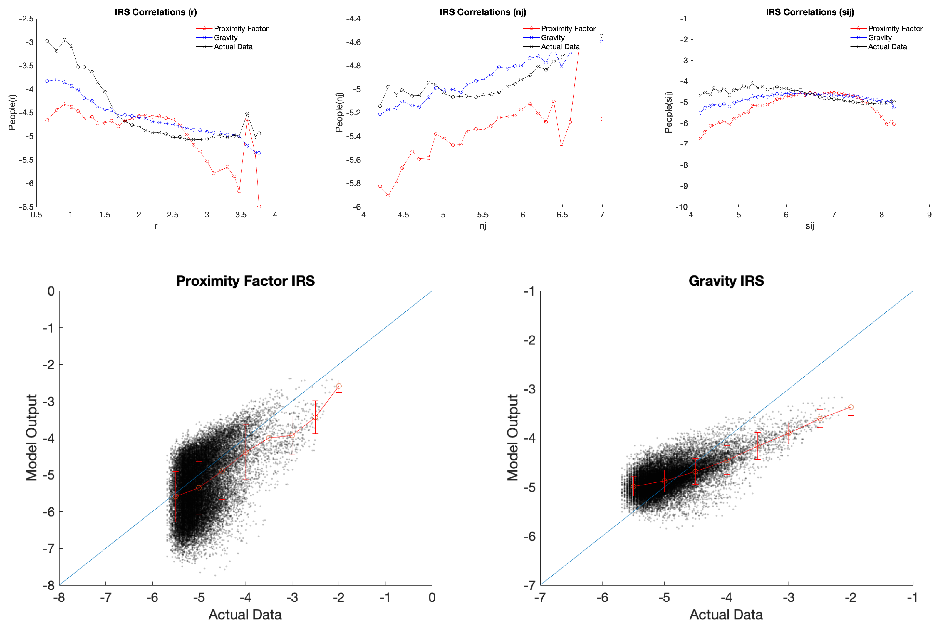
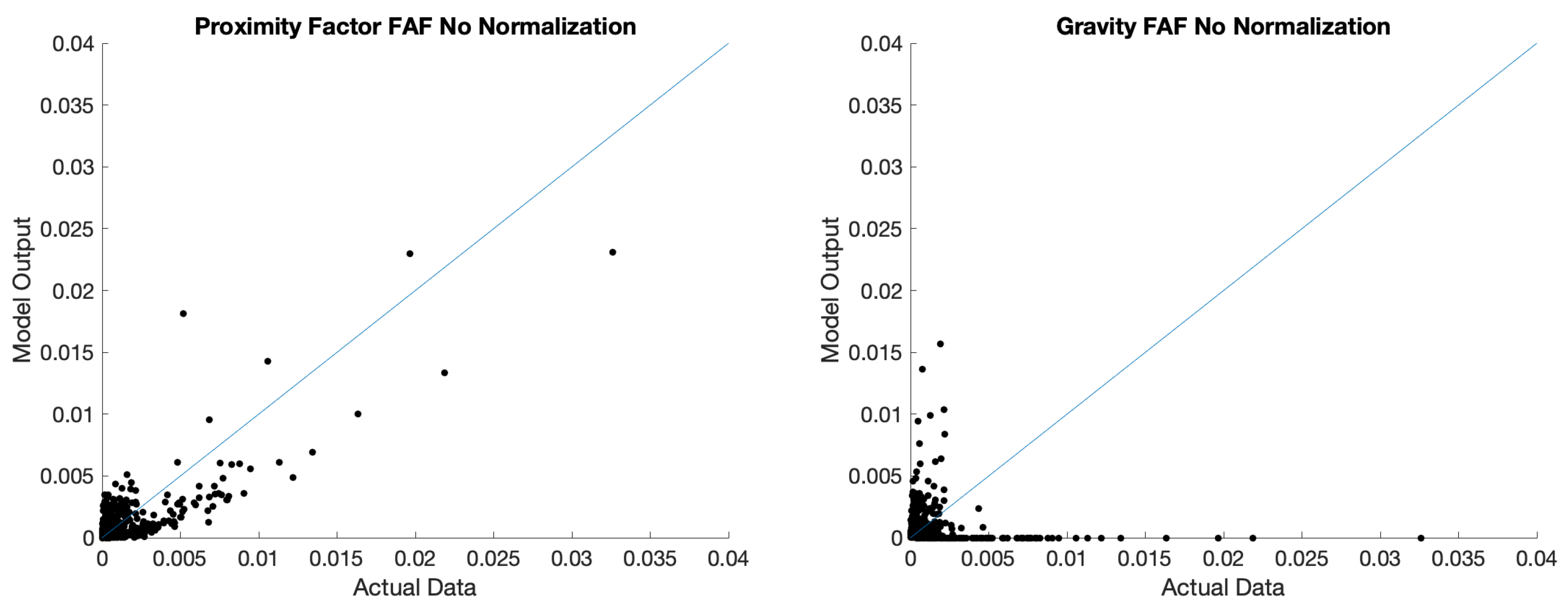
We compared the two models in a home delivery logistics network design algorithm [23]. This algorithm tries to find the best distribution center (DC) location in a city for consolidated package delivery. Packages enter the system from the vendors’ warehouse and trickle to the closest DC to the end customer. In addition to the existing customer demand, the linehaul between DCs creates extra package inflow and outflow in DCs. We needed a way to calculate demand flows to find the linehaul. Hence, we decided to try both the proximity factor and the gravity models in this algorithm.

Both models seem to be compatible with the algorithm. However, the proximity factor works more smoothly compared to the gravity model. Also, the gravity model provided a lot of inefficient and infeasible solutions as DCs struggled to maintain the required utilization levels between 90% and 110%. The reason behind this is the huge difference between low and high interaction outputs for the gravity model. The proximity factor model has a smoother transition from the low and high interactions. Additionally, the gravity model outputs are more heterogeneous causing the algorithm to fail in several instances. Finally, the gravity model takes a longer time to run than the proximity factor model. This makes the proximity factor model a better model to calculate demand flows in this algorithm.

4. Validation

In this section, we tested the models defined in Equations (2) and (8) against empirical data. We used the US Department of Transportation’s Freight Analysis Framework (FAF) data [24]. FAF provides us with how much freight (or commercial goods) is transported between FAF zones. There are 132 FAF zones throughout the US. As a result, origin and destination points are not clearly defined, which makes the granularity of the data a bit low. However, this is the only dataset that gives us insight into the commodity flow in the United States.

The data were collected by the US Department of Transportation and had the freight transportation information that had occurred in the country between 2012 and 2017 [24]. FAF zones consist of major metropolitan areas with high population density regions and state or rest of the state for low population density regions. There are no multi-state zones in this dataset.

Besides the O-D pairs, the data also include the amount of freight traveled between these points as tons and ton-miles. However, there were some gaps in our distance matrix as some zones did not have commodity transfers. These gaps were filled with the data acquired from Google Maps. We calculated the distances between O-D pairs by dividing ton-miles by tons. Since the number of FAF zones was small enough to calculate the entire country, we did not focus on a particular region. We also used the data from the 2007–2012 databases for comparison purposes.

Our analysis concludes that the proximity factor is superior to the gravity model. $R^2$ values indicate that the proximity factor could explain 59.19% of the variation in data, whereas the gravity model is in the range of 0.93%. In addition to that $RMS{E}_P$ is $3.374\times {10}^{-4}$ and $RMS{E}_G$ is $6.969\times {10}^{-4}$, showing less error for the proximity factor. The main reason for the differences between $R^2$ and $RMSE$ values might be the distance calculation. Hence, we wanted to explore different distance calculations to give the gravity model a better chance. In the FAF data, distance is calculated using the data provided (ton-miles divided by tons), but we could not find a satisfactory explanation of how the ton-miles portion of the data is calculated. Thus, we decided to calculate the distances between zones on our own. We found a list with county information for all the FAF zones. Using their FIPS codes and Matlog’s uscounty database [25], we calculated the geographical centers of all zones. Next, we used the great-circle distances to calculate distances between O-D pairs. This method neither changed the $R^2$ results for the proximity factor nor the gravity model, as the former was around 0.54 and the latter was still at 0.00.

When we look at the correlations in the top panel of Figure 4, the proximity factor is faring better with distance r than the gravity model. However, the gravity model gets better with increasing r values. The destination population correlations, in this case, the ton value, $n_j$, show us that both the proximity factor and the gravity model are not doing well. $s_{ij}$ correlations also show no indication of the superiority of one model over the other. In some cases, the proximity model shows better results, while in others, the gravity model results are better. All the plots are in log-log scale, so the correlations are in the form of power laws.

In the middle panel of Figure 4, we analyze the freight transportation routes between the zones. Here, we show a scatter plot comparison between the actual data (x axis) and the model’s output (y axis). Moreover, we show the mean in red circles, standard deviation bars, and the x = y line to show where the model meets the actual data. All the plots in this panel are also in the log-log scale. We can see that the proximity factor is more accurate than the gravity model, but the precision is lower for the proximity factor. Both models get better with higher ton values, but the proximity factor’s accuracy increases substantially compared to the gravity model. However, these graphs can be misleading. Hence, we added the actual scatter plots in the bottom panel; the proximity factor’s ability to predict the actual data can be successfully seen there. The noise at the bottom left section caused the log-log scale to clutter unnecessarily.

5. Discussion

There are multiple aspects to the synthetic demand generation problem. Various models have been proposed recently, but the gravity model is still considered the best option to handle this problem. The proximity factor’s independence from the metric distance and the fact it requires fewer parameters than conventional models, such as the gravity model, is a significant and desired change.

In this paper, we address the compatibility and reliability of the proximity factor against the gravity model for different datasets. The first thing we noticed was that the dynamics of the dataset play a considerable role for most models in computing the flows. If there are flow patterns, models do not fare well with that particular dataset.

There are also some structural problems associated with the gravity model. It changes drastically with the change in distances and cannot calculate the same point interactions where the distance is zero. The gravity model’s use of past data is another problem. It tries to imitate past data but cannot absorb the abrupt changes happening in the moment. The proximity factor does not require a past dataset to use in applications. This gives a considerable advantage. The robustness of the proximity factor is shown in the model comparison section.

Despite its satisfactory performance, the proximity factor can be further improved. Its flow ranking algorithm can be improved to reflect other environmental changes, such as changing it from order ranking to distance ranking. In this regard, a new universal visitation law has been proposed recently [26]. The inverse correlation between the multiplication of distance and population density can be integrated into the proximity factor. However, the universal visitation law considers the probability of visitation for individuals, whereas the proximity factor calculates the likelihood of demand flows. As a result, we believe this integration would be out of the scope of this paper. In certain instances where distance between O-D pairs might play a huge role in determining the flow density (multi-modal applications, possibly), the gravity model could be preferable over the proximity factor due to gravity model’s reliance on distance.

Another further improvement could be the investigation of the universality of the proximity factor. Analyzing its implementation in different settings and environments would prove whether it is universal or not. A comparison between the two models for maximum distances in the dataset can further solidify the robustness of the proximity factor.

References

1. Kay, M.G.; Parlikad, A.N. Material Flow Analysis of Public Logistics Networks. In Progress in Material Handling Research; Meller, R., Ogle, M., Peters, B., Taylor, D., Usher, J., Eds.; The Material Handling Institute: Charlotte, NC, USA, 2002. [Google Scholar]
2. Kay, M.G.; Warsing, D.P. Estimating LTL rates using publicly available empirical data. Int. J. Logist. Res. Appl. 2009, 12, 165–193. [Google Scholar] [CrossRef]
3. Cordeau, J.F.; Pasin, F.; Solomon, M.M. An Integrated Model for Logistics Network Design. Ann. Oper. Res. 2006, 144, 59–82. [Google Scholar] [CrossRef]
4. Melo, M.T.; Nickel, S.; Saldanha-Da-Gama, F. Facility Location and Supply Chain Management—A Review. Eur. J. Oper. Res. 2009, 196, 401–412. [Google Scholar] [CrossRef]
5. Guo, W.; Toader, B.; Feier, R.; Mosquera, G.; Ying, F.; Oh, S.W.; Price-Williams, M.; Krupp, A. Global Air Transport Complex Network: Multi-Scale Analysis. SN Appl. Sci. 2019, 1, 1–14. [Google Scholar] [CrossRef]
6. Hua, C.; Porell, F. A Critical Review of the Development of the Gravity Model. Int. Reg. Sci. Rev. 1979, 4, 97–126. [Google Scholar] [CrossRef]
7. Balcan, D.; Colizza, V.; Gonçalves, B.; Hu, H.; Ramasco, J.J.; Vespignani, A. Multiscale Mobility Networks and the Spatial Spreading of Infectious Diseases. Proc. Natl. Acad. Sci. USA 2009, 106, 21484–21489. [Google Scholar] [CrossRef] [PubMed]
8. Kalahasthi, L.; Holguín-Veras, J.; Yushimito, W.F. A Freight Origin-Destination Synthesis Model with Mode Choice. Transp. Res. Part E Logist. Transp. Rev. 2022, 157, 102595. [Google Scholar] [CrossRef]
9. Holguín-Veras, J.; Patil, G.R. Integrated Origin–Destination Synthesis Model for Freight with Commodity-Based and Empty Trip Models. Transp. Res. Rec. 2007, 2008, 60–66. [Google Scholar] [CrossRef]
10. Holguín-Veras, J.; Patil, G.R. A Multicommodity Integrated Freight Origin–Destination Synthesis Model. Netw. Spat. Econ. 2008, 8, 309–326. [Google Scholar] [CrossRef]
11. Erlander, S.; Stewart, N.F. The Gravity Model in Transportation Analysis: Theory and Extensions; VSP: Leiden, The Netherlands, 1990. [Google Scholar]
12. Zipf, G.K. The P1 P2/D Hypothesis: On the Intercity Movement of Persons. Am. Sociol. Rev. 1946, 11, 677–686. [Google Scholar] [CrossRef]
13. Barbosa, H.; Barthelemy, M.; Ghoshal, G.; James, C.R.; Lenormand, M.; Louail, T.; Menezes, R.; Ramasco, J.J.; Simini, F.; Tomasini, M. Human Mobility: Models and Applications. Phys. Rep. 2018, 734, 1–74. [Google Scholar] [CrossRef]
14. Simini, F.; González, M.C.; Maritan, A.; Barabási, A.L. A Universal Model for Mobility and Migration Patterns. Nature 2012, 484, 96–100. [Google Scholar] [CrossRef] [PubMed]
15. Masucci, A.P.; Serras, J.; Johansson, A.; Batty, M. Gravity versus Radiation Models: On the Importance of Scale and Heterogeneity in Commuting Flows. Phys. Rev. E 2013, 88, 022812. [Google Scholar] [CrossRef] [PubMed]
16. Lenormand, M.; Bassolas, A.; Ramasco, J.J. Systematic Comparison of Trip Distribution Laws and Models. J. Transp. Geogr. 2016, 51, 158–169. [Google Scholar] [CrossRef]
17. Jung, W.S.; Wang, F.; Stanley, H.E. Gravity Model in the Korean Highway. EPL Europhys. Lett. 2008, 81, 48005. [Google Scholar] [CrossRef]
18. Yang, Y.; Herrera, C.; Eagle, N.; González, M.C. Limits of Predictability in Commuting Flows in the Absence of Data for Calibration. Sci. Rep. 2014, 4, 5662. [Google Scholar] [CrossRef] [PubMed]
19. Joines, J.A.; Houck, C.R. On the use of non-stationary penalty functions to solve nonlinear constrained optimization problems with GA’s. In Proceedings of the First IEEE Conference on Evolutionary Computation. IEEE World Congress on Computational Intelligence, Orlando, FL, USA, 27–29 June 1994; pp. 579–584. [Google Scholar]
20. De Dios Ortúzar, J.; Willumsen, L.G. Modelling Transport; John Wiley & Sons: Hoboken, NJ, USA, 2011. [Google Scholar]
21. Mathai, A.M. An Introduction to Geometrical Probability: Distributional Aspects with Applications; CRC Press: Boca Raton, FL, USA, 1999. [Google Scholar]
22. Wilson, R.A. Transportation in America: Statistical Analysis of Transportation in the United States. Historical Compendium 1939–1995; Eno Transportation Foundation: Westport, CT, USA, 2002. [Google Scholar]
23. Yalvac, E. Design of a Home Delivery Logistics Network. Ph.D. Dissertation, North Carolina State University, Raleigh, NC, USA, 2023. [Google Scholar]
24. Department of Transportation Freight Analysis Framework. Available online: https://faf.ornl.gov/faf5/ (accessed on 18 March 2021).
25. Kay, M.G. Matlog: Logistics Engineering Using Matlab. J. Eng. Sci. Des. 2016, 4, 15–20. [Google Scholar]
26. Schläpfer, M.; Dong, L.; O’Keeffe, K.; Santi, P.; Szell, M.; Salat, H.; Anklesaria, S.; Vazifeh, M.; Ratti, C.; West, G.B. The Universal Visitation Law of Human Mobility. Nature 2021, 593, 522–527. [Google Scholar] [CrossRef] [PubMed]
27. US Census Bureau Commuting Data Statistics. Available online: https://www.census.gov/topics/employment/commuting/data.html (accessed on 31 December 2020).
28. Internal Revenue Service SOI Tax Stats—Migration Data. Available online: https://www.irs.gov/statistics/soi-tax-stats-migration-data (accessed on 23 February 2021).
29. Bureau of Transportation Monthly Transportation Statistics. Available online: https://data.bts.gov/stories/s/m9eb-yevh (accessed on 30 November 2020).
30. Liu, S.; Su, Y. The Impact of the COVID-19 Pandemic on the Demand for Density: Evidence from the US Housing Market. Econ. Lett. 2021, 207, 110010. [Google Scholar] [CrossRef]
Figure 1. Spencer−Spirit Lake, IA CSA data points.
Forecasting 07 00014 g001
Figure 2. CSA data points for Gainesville−Lake City, FL, Raleigh−Durham, NC, and Atlanta, GA.
Forecasting 07 00014 g002
Figure 3. Error comparison of Gainesville run: average error comparison in the left, diagonal points error comparison in the middle, and non-diagonal error comparison in the right.
Forecasting 07 00014 g003
Figure 4. Analysis results for FAF data. Top panel FAF5 2012−17. Parameters for the single parameter gravity model: γ = 2.5346.
Forecasting 07 00014 g004aForecasting 07 00014 g004b