Abstract
Wind data are often cyclostationary due to cyclic variations, non-constant variance resulting from fluctuating weather conditions, and structural breaks due to transient behaviour (due to wind gusts and turbulence), resulting in unreliable wind power supply. In wavelet hybrid forecasting, wind prediction accuracy depends heavily on the decomposition level () and the wavelet filter technique selected. Hence, we examined the efficacy of wind predictions as a function of and wavelet filters. In the proposed hybrid approach, differential evolution (DE) optimises the decomposition level of various wavelet filters (i.e., least asymmetric (LA), Daubechies (DB), and Morris minimum-bandwidth (MB)) using the maximal overlap discrete wavelet transform (MODWT), allowing for the decomposition of wind data into more statistically sound sub-signals. These sub-signals are used as inputs into the gated recurrent unit (GRU) to accurately capture wind speed. The final predicted values are obtained by reconciling the sub-signal predictions using multiresolution analysis (MRA) to form wavelet-MODWT-GRUs. Using wind data from three Wind Atlas South Africa (WASA) locations, Alexander Bay, Humansdorp, and Jozini, the root mean square error, mean absolute error, coefficient of determination, probability integral transform, pinball loss, and Dawid-Sebastiani showed that the MB-MODWT-GRU at was best across the three locations.
Keywords:
wind speed; wind forecasting; MODWT; differential evolution; GRU; Morris minimum bandwidth 1. Introduction
1.1. Research Motivation
Wind power is clean and environmentally friendly. Furthermore, wind power has multiple economic and societal advantages [1,2,3,4]. For instance, wind power is economical, sustainable, and inexhaustible [1,2,3,4,5]. In fact, wind power resources are abundant, and can be captured day and night (when solar energy is unavailable). Consequently, there has been a rapid increase in the volume of wind power penetrating existing electric power grids. Provided that the primary and most significant input or resource to wind power, namely, wind speed, is highly complex and unpredictable, the integration of substantial amounts of wind power into the power grid frequently compromises wind power management strategies [5].
The complex nature of wind speed originates from the fact that wind as a physical quantity is dependent on a variety of complex factors, such as atmospheric pressure fluctuations, topography changes, seasonal variations, elevation above ground level, weather patterns, and land formations, such that it is irregular and variable in both location and time scale [3,4]. Furthermore, wind data display cyclostationarity due to unsteady cyclic variations, non-constant variance from changing weather phenomena, and structural breaks reflecting transient wind behaviour [6], which could be handled (or extracted) through the proper utilisation of denoising approaches [7,8] such as wavelet transforms (WTs).
Theoretically, wind power increases eightfold when wind speed doubles. However, in practice, wind turbine output is constrained beyond certain speed limits (i.e., cut-out speed) [4]. As a result, errors in estimating wind speed can lead to significant fluctuations in pricing and missed investment opportunities in the energy markets [8,9]. Therefore, studying the availability of wind and the resulting generation of wind power is essential for informed management and investment decisions in electricity markets. Overall, handling wind speed data, a multi-dimensional (encompassing nonlinear and linear behaviour) and ever-changing physical phenomenon, using a single model often leads to inaccurate and unreliable predictions.
1.2. Literature Highlights
It is pivotal to use models that predict wind speed with high accuracy to improve and properly regulate wind power output. Although physical models can effectively predict atmospheric dynamics, they require the use of large amounts of numerical weather data, hence the need for longer training time to correlate various datasets [9,10]. On the other hand, statistical models (e.g., autoregressive integrated moving average (ARIMA)) are generally reserved for capturing short-time and linear data characteristics, as they are insufficient for capturing nonlinear ones and longer forecast horizons [10]. The advancement of technology in recent years has resulted in machine learning methods (which are mostly data-greedy and black-boxed), dominating both statistical and physical methods in tuning speed, scalability, and accuracy when handling high-variant, nonlinear stochastic, and non-stationary wind speed sequences, as well as achieving robustness and efficiency, and thus attracting considerable interest.
Hybrid models combine more than one forecasting method to form a new one, thereby addressing the deficiencies of each single model by harnessing each model’s strengths [6,11]. The high precision, accuracy, and, to some extent, processing power of hybrid techniques have garnered significant attention from researchers in recent years. Additionally, the combined approaches are excellent at handling and overcoming frequent statistical, computational, and representational drawbacks in the forecasting arena [9,11]. In short-term wind speed forecasting, the authors of [12] combined artificial neural networks (ANNs) with WT to develop WT-ANN. The proposed approach using the Daubechies 4 (DB4) filter demonstrated superior wind forecasting power compared to the model without wavelet transformation. In a similar approach to that of [12], the authors of [13] used the discrete wavelet transform-ANN (DWT-ANN) (DB4) to predict wind speed on a short-term horizon with high accuracy. In the work of [14], the authors propose WD-NILA-WRF, a combination of wavelet decomposition (WD) and weighted random forest (RF) (WRF), based on the niche immune lion algorithm (NILA) for ultra-short wind speed forecasting. Based on 10 min interval wind speed data, the work of [15] combined WT (DB3), ARIMA, and machine learning algorithms (support vector regression (SVR) and RF), which showed promising wind speed forecasting results. According to the authors of [10], the repeated WT-ARIMA (RWT-ARIMA) approach based on (DB2) improved very short-term wind speed forecasting significantly. In the work of [4], similar results were obtained through the application of least asymmetric 8 (LA8) maximal overlap discrete wavelet transform (MODWT), ARIMA, gradient-boosting decision trees (GBDTs), and SVR for short-term wind speed forecasting. The authors of [16] also proposed an effective hybrid strategy that combines (DB4) WT, particle swam optimisation (PSO), and an adaptive neuroma-fuzzy inference system (ANFIS) to significantly and effectively reduce wind power prediction errors on a short-term forecast scale. The work of [17] (DB4) and [18] (DB7) combined DWT with long short-term memory (LSTM) networks for short-term wind speed forecasting. Despite the lengthy processing time for LSTM, the results showed that WT preprocessing significantly improved forecast accuracy. In a similar study, the work of [19] enhanced short-term wind speed predictions using a hybrid approach that combines LA8, MODWT, sample entropy, neural network autoregression (NNAR), LSTM and gradient boosting machine (GBM). Although highly accurate and robust, LSTMs were found to be computationally expensive.
None of the studies reviewed above provided adequate rationale for selecting the specific type of wavelet filter and decomposition level. Additionally, most studies used a single-wavelet filter (especially DB) in the data pre-processing phase, with very scant usage of Morris minimum bandwidth (MB). Aside from [19], the examined research papers hardly explored MODWT, or the strategy used to determine the level of decomposition in detail. Rather than using a reproducible mathematical approach, the level of decomposition is often determined by trial and error (see e.g., [10,12,13]).
In wind speed forecasting, ref. [20] applied wavelet filters (such as DB and LA) to various forecasting models (i.e., persistence, neural networks (NNs), fuzzy logic, and regression) across different decomposition levels. Additionally, the study discarded high-variant detailed frequency components, only forecasting the original signal from smooth approximation sub-signal. It was found that the decomposition level (optimised using a genetic algorithm (GA)) significantly influenced the results, more so than the choice of wavelet filter. In a similar work, the authors of [21] proposed a GA-optimised wavelet neural network (WNN) for day-ahead wind speed forecasting, which outperformed traditional wavelet-based forecasting techniques in precision. The aforementioned studies used simple statistical models that are prone to nonlinearity, or conventional ANNs that are susceptible to vanishing gradients and overfitting (see e.g., [12,13,20,21]).
The application of differential evolution (DE) as a metaheuristic search algorithm for the optimisation of wavelet decomposition levels in wind speed forecasting is seldom (or never) addressed in the existing literature compared to GA. Furthermore, most of the studies (see e.g., [12,13]) used the conventional DWT, which (though effective) is shift-variant such that miniature changes in the signal affect wavelet coefficients compromising their ability to effectively undertake time series tasks as compared to the more effective and time-invariant MODWT (see [19]). In general, there is scant literature on the choice of wavelet methods and decomposition levels used in wind forecasting, compromising the comparability and reproducibility of the results.
Hence, this study proposes a hybrid wavelet-MODWT-GRU approach to effectively assess the influence of the wavelet filter and decomposition level on the accuracy and reliability of wind predictions. This approach leverages the strengths of MODWT, which effectively denoises highly variable signals and exposes transient wind behaviour, along with DE, recognised for its strong global search capabilities, fast convergence, and simplicity. Thus, our proposed approach uses DE to optimise the decomposition levels of the DB, LA, and MB wavelet filters. This enables the efficient decomposition of wind speed signals into frequency components with improved statistical characteristics, facilitating the detection of cyclic changes in the mean and variance using MODWT. Each sub-signal from the MODWT decomposition is individually forecasted using the GRU model to effectively capture the complex behaviour of wind speed. The final predicted value is derived by reconstructing the original signal using the inverse MODWT method based on a multiresolution analysis (MRA) technique that incorporates each sub-signal forecast as input. We compared the performance of three wavelet-MODWT-GRU models, LA-MODWT-GRU, DB-MODWT-GRU, and MB-MODWT-GRU, using 10 min averaged high-resolution wind speed data from Alexander Bay, Humansdorp, and Jozini stations from the Wind Atlas South Africa (WASA) (https://wasadata.csir.co.za/wasa1/WASAData) (accessed on 20 September 2022/5 June 2023). We further evaluated the efficacy of the best wavelet-MODWT-GRU among the three models against the GRU model and the benchmark naïve model, using deterministic and probabilistic predictions.
1.3. Innovations
The novelty and originality of the proposed ensemble method are postulated on the basis that wind data are characterised by cyclostationarity due to cyclic variations, non-constant variance resulting from fluctuating weather conditions, and structural breaks that reflect transient wind behaviour [6,7]. As such it cannot be effectively and efficiently characterised by one single class of model.
Unlike Fourier transforms (FT), the proper selection of wavelets can accurately identify structural breaks, thereby enhancing the accuracy and reliability of wind speed forecasting [7]. However, the prior application of the wavelet-based classes of hybrid models focused on prediction accuracy, disregarding significant elements of wavelets specifically the selection of the decomposition level and type of wavelet filter [8], which ultimately and holistically influence the level of accuracy and reliability of the wind predictive model [12,20,21].
Deterministic prediction metrics (i.e., root mean square error (RMSE), mean absolute error (MAE), and mean absolute percentage error (MAPE)) have been the top priority in the wind forecasting literature [10,14,15,16,20,21], and are constantly being refined to make them more accurate. However, in extreme and uncertain conditions, these forecasts cannot completely capture the chaotic nature (i.e., wind gusts and turbulence) of wind speed. Consequently, the sporadic gap between observed and predicted values can pose risks to wind power market scenarios. Thus, our motivations are summarised as follows:
- We choose wavelets because they efficiently manage complex wind data by decomposing signals into different frequency components, allowing for the detection of complex patterns. In essence, we used wavelets to accurately identify structural breaks, thereby enhancing the accuracy and reliability of the wind speed forecasting model.
- Instead of using the time-variant DWT, we opted for MODWT, which is time-invariant such that subseries signals have the same coefficients even if the signal is shifted [3,8,19]. Plus, these methods maintain the full resolution of the original signal as it does not apply a decimation, thereby enhancing the modelling and forecasting of sub-signals. We, therefore, used the MODWT technique to decompose the original wind speed data signal into detailed and approximate frequency sub-signals with reduced complexity than the original sub-signal.
- The selection of the most suitable wavelet filter depends on the specific problem being addressed. In contrast with conventional DB4 and LA8, we also applied MB filters exhibiting excellent frequency localisation, narrow bandwidths reducing spectral leakage, and the effective isolation and filtering of noise outside a particular frequency band [22].
- GA results are reliable and consistent, but these algorithms require significant computational resources and are typically characterised by a slow convergence rate. DE differs from GA in that it can solve complex optimisation problems and optimise non-differentiable and nonlinear continuous functions with high convergence speed, making it well suited to forecasting wind speeds [23,24,25,26]. We utilised the latter stochastic algorithms, which are easy to understand and converge quickly, to find the optimal level of decomposition for the wavelet filter applied.
- Often, wind speed (as a physical quantity) presents itself at particular locations in both linear and nonlinear forms, which compromises the performance of linear models in the forecasting arena. GRUs have the ability to capture varying patterns of variance over time which is typical of wind data. By leveraging GRU’s simplicity, accuracy and computational efficiency (to some extent), we modelled and predicted each sub-signal to such a level of accuracy and precision.
- Also, most reviewed studies focused on short-term forecasts (see e.g., [10,12,13,14,15,16,17,18,19,20]), ignoring the medium-to-long-term forecasts that are critical to wind turbine maintenance and wind farm construction. We evaluated probabilistic or distributional forecast measures in both medium and long-term wind speed forecasting using pinball loss (PL), Dawid–Sebastiani (DS), and probability integral transform (PIT).
- The practicability and efficacy of the proposed forecasting model were confirmed empirically via prediction metrics. Also, this work was conducted in a way that is reliable and easy to replicate.
1.4. Structure of the Study
2. Materials and Methods
2.1. Fundamentals of Wavelet Analysis
A wavelet is a compact wave that can adjust its amplitude and width within a fixed time frame [3,27,28,29,30,31]. Unlike FTs, which focus primarily on sine waves, wavelet analysis utilises a broader range of functions. Its distinctive properties make it well-suited to various problems, allowing for customisation of parameters based on specific requirements [3,30,31]. In fact, wavelet analysis is capable of localised and MRA, enabling the identification of trends, structural breaks, and discontinuities that may be overlooked by other methods such as FT and short-time Fourier transform (STFT) [3,27,31]. Furthermore, wavelets’ support for MRA provides a greater flexibility advantage over STFT and FT. In addition, wavelets can analyse frequency and time simultaneously, unlike FTs, which can only analyse either time or frequency [3,18,21]. In essence, wavelets are actually real-valued mathematical functions defined in real space such that they satisfy two main fundamental properties [3], namely
Wavelets are widely employed in discrete DWT, but also in continuous WT (CWT). The CWT and DWT are, respectively, given by the following equations:
where denotes the conjugate of with being a scaling factor and a time-shifting parameter. The current study will focus on the application of the MODWT in the context of wind speed forecasting.
2.1.1. Wavelet Filters
DB wavelets are orthogonal; however, they are not symmetrical [28,29,30,31,32]. The scaling functions for DB wavelets have regularity properties such that it has compact support, and can accurately decompose and recompose signal functions [28,31]. Symlets (e.g., least asymmetric) are also orthogonal and compactly supported wavelets, which were proposed by [28] as modifications to the conventional DB. This filter offers symmetry and regularity beyond that of traditional DB wavelets, which facilitates signal reconstruction with minimal signal distortion [28,31]. In fact, their high regularity and symmetrical properties enable precise feature extraction while minimising noise [28,29,30,31]. The MB wavelets minimise frequency bandwidth while retaining their localisation properties, making them suitable for signal denoising and data extraction. Furthermore, this wavelet filter is less susceptible to spectral leakages in frequency domain applications [22] (also see Table 1).

Table 1.
Properties of wavelet filters applied in the current study.
Overall, the DB filter is ideal for signals with sharp transitions, but might be less effective for high-frequency analysis. The LA filter offers a balanced option for mixed signals, while the MB filter excels in high-frequency analysis and minimises spectral leakage, making it particularly useful for wind speed forecasting.
2.1.2. Multiresolution Analysis
In MRA, a signal is broken down into components with better statistical properties, which are then combined to reconstruct the original signal. The advantage of MRA is that features can be localised in both time and frequency. In wind speed predictions, this helps identify transient wind behaviour such as wind gusts, thereby improving overall model accuracy and precision. The MRA equation for the wind speed signal is given by [28,31,35]
where is approximate or scaling coefficients at the resolution level , and denotes the detailed coefficients for each level and position . As a result of this decomposition, a structured view of a signal is gained, which allows for efficient compression, denoising, and feature extraction [28,31]. An essential component of the MRA technique is the ability to efficiently decompose and reconstruct the original signal.
2.1.3. Maximal Overlap Discrete Wavelet Transform
MODWT is a version of DWT [7,19,33,34,35]. Similar to conventional DWT, these methods utilise both MRA and pyramid algorithms to decompose signals into approximate and detailed sub-signals of varying scales with more exposed trends and patterns [33,34,35]. While DWTs allow for signal-perfect reconstruction, they decimate (downscale) the signal, resulting in sub-signals with smaller coefficients than the original signal [33]. Furthermore, these techniques are shift-variant in the sense that miniature changes in the signal affect wavelet coefficients, making them (to some extent) unfit for complex time series exercises such as wind speed forecasting. MODWTs are time-invariant and maintain the original signal’s full resolution because they do not use a decimation approach [7,33,34,35]. Different from conventional DWT, MODWT improves wavelet strength by altering the filter, not the signal, making it more resistant to boundary effects [33,34,35]. As such, MODWT has better statistical stability than DWT and can handle quasi-stationary signals such as wind speed data. Consider the time series signal decomposed into several detailed signals {} and an approximate signal {}. Then, the MRA representation for
MODWT is given by (see [35] for details)
where is the length of the wavelet filter; ; and , respectively, denote the scaling and wavelet filter coefficients of a band-pass filter (critical for energy conservation). The equations above must satisfy the following conditions (see [35] for details):
This is a pivotal property for the perfect reconstruction of the signal. Using the inverse pyramid algorithm, the original signal can be reconstructed through the following mathematical expression [7,35]:
Thus, the wavelet and scaling coefficients are calculated by cascading convolutions with filters and [35]. It should be noted that at each resolution level (see [35] for details).
2.2. Differential Evolution
DE is a stochastic algorithm that can be applied to complex optimisation problems without explicit adaptation to each particular problem [23]. Furthermore, DE is effective and efficient at minimising non-differentiable and possibly nonlinear continuous functions [23,24,25]. In this way, DE is more reliable, robust, efficient, accurate, and scalable than artificial bee colony (ABC), simulated annealing (SA), GA, and PSO (also see [23,24,25]). The four main steps involved in the DE algorithm are detailed below.
Step 1: Intialisation
Consider an objective function. Ideally, we seek to find a solution such that for all with the boundary constraints where . DE uses population which consists of potential solutions to explore a solution space. The DE starts by initialising the population such that the initial population with random initialisation given by [23,24]:
where and , respectively, denote the lower and upper limit, and is a uniform distribution. In essence, each element or individual in the population is uniformly distributed within a multidimensional search space. By substituting superior individuals in the present population for every generation, the algorithm builds a new population. To reach the global minimum, the population will have to go through mutation, crossover, and selection processes [23,24,25,26].
Step 2: Mutation
The mutation is a biologically inspired terminology which enables the algorithm to effectively and efficiently effect random modification on the population by developing the so-called mutant vector for each individual in the population [23,24,25,26]. To form a mutant or donor vector (), the three distinct population individuals are randomly selected from the population. Thereafter, the scaled differences (accounting for differential fluctuations) of the distances between any two of the three vectors are summed to the third one such that [24,25]
where represents a mutant vector for the ith individual in the next generation (); and are distinct individuals (i.e., ) randomly and independently selected from the population generation ; and denotes the scaling factor. In the DE/rand/1 presented in Equation (13), each mutant step blends parameter sets between successful population individuals. As shown in Equation (14), most DE strategies apply pairs of difference vectors (see [24,25] for details):
where such that substituting the best vector ( from the population will yield the DE strategy given by the equation below:
Using scaled difference vectors and a weighted average of the best and arbitrary vectors, DE mutant strategies can be generally represented by the following equation [23,24,25]:
Step 3: Crossover
The crossover operator creates offspring by mixing components of the current element and those generated by mutation [24,25,26]. The elements of the mutant vector are transferred to the trial vector with a certain probability (. In essence, the binomial crossover parameter mixes either the characteristics of the mutant () and target vector () to develop a trial vector strategy () such that [23,24,25,26,36]
where are uniformly distributed random numbers generated for each and , and denotes the crossover probability initialised from the start. The parameter is vital as it assures that . High encourages exploitation through a broader search space, whereas low emphasises refinement. In addition to ensuring escape from local maxima, crossing ensures that the algorithm is able to make bigger steps across the problem landscape [26,36,37].
Step 4: Selection
In the final step, the trial vector is compared with the target vector , and the vector with the optimal function value is propagated to the next generation [26,36,37] such that
where is the objective function. Thus, if the new trial vector (i.e., ) is the same or smaller than the target vector, it becomes the new target. If not, the target vector stays the same, thereby ensuring that the population remains the same or improves [23,24,25,26,36,37]. The mutation, crossover and selection carry on until some termination criteria are attained.
In the “DEoptim” package of the R program (version 4.4.1), we applied the DE/rand/1/bin strategy (discussed above) to optimise the decomposition level (also see [38]).
2.3. Gated Recurrent Unit
The GRU is a simpler and more efficient variant of recurrent neural networks (RNNs) designed for processing sequential data of variable length; it is not prone to the vanishing gradient problem that affects conventional neural networks [39,40,41]. Different from LSTMs, GRUs have a much simpler structural architecture. Provided that the parameters are kept the same, the work of [41] showed that GRUs could outperform LSTMs in terms of convergence, computational time, parameter updates, and generalisation on varying datasets. Comparable to LSTM, GRU interpolates the previous hidden state () and candidate hidden state () to build an activation function such that [41]
where denotes element-wise multiplication, the update gate at controls how much information from the hidden state should be retained and is given by the following expression:
where is the input at time , is the hidden state from the previous time step, and denote weight matrices, is the logistic sigmoid function given by:
It should be noted that will mostly retain information from , otherwise will retain information The candidate activation () is given by the following equation:
where the reset gate is given by the following expression which is similar to that employed by the update gate:
where is the reset gate at time , and are weight matrices associated with the reset gate. This equation governs the extent to which the previous hidden state is disregarded when calculating the new candidate’s hidden state [41]. With varying datasets, GRUs can capture temporal trends and dependencies, but they may fall behind LSTMs (which can handle highly complex sequential data) in time series tasks involving long-term dependencies (see [41]). We fitted the GRU using the “keras” library in the R program.
2.4. Persistence Model
The naive model assumes that the wind speed data at the time is exactly the same as it was at the time Generally, the naive model is used as a benchmark model, and it provides accurate forecasts for short and very short-term forecasting timescales [42]. The naive model is given by the equation below:
2.5. Proposed Prediction Approach
The wind speed data are characterised by continuous variation and structural breaks resulting from transient wind behaviour, which negatively impacts the integration of large volumes of wind power into the existing power grid and is difficult to capture using a single forecasting model. In turn, the resultant power disequilibrium complicates the operation of power grids and utility managers’ ability to develop effective management strategies. A methodology for improving wind speed forecasting is depicted in Figure 1 which outlines the sourcing, cleaning and processing of data, as well as the use of evolutionary algorithms, wavelets, and machine learning algorithms. Hence, we summarise the role of each of the models involved in the development of the optimised wavelet-MODWT-GRU model as follows (also see Algorithm 1):
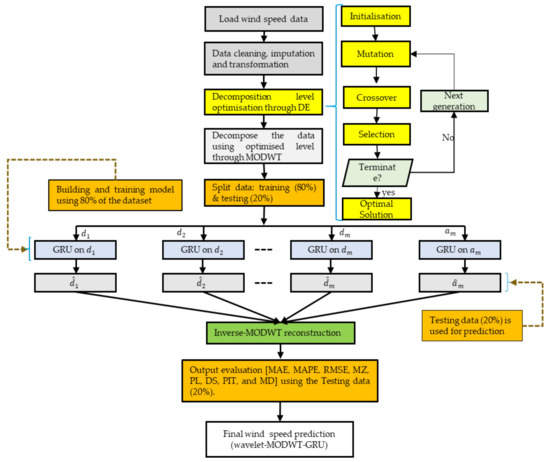
Figure 1.
Flow chart of the proposed wavelet-MODWT-GRU.
- DE algorithm is used to optimise the decomposition level of highly variant wind speed data due to its simplicity, efficiency, and ability to deal with complex continuous non-differentiable problems. As a result, more statistically sound sub-signals that are easy to characterise in modelling and forecasting can be extracted.
- A time-invariant MODWT resistant to boundary effects is used, employing a variety of wavelet filters, particularly the DB4, LA8, and MB8, to decompose wind speed data into detailed (high) and approximate (low) frequency components. These components have reduced noise and volatility, exposing short-term and long-term trends. They can be modelled and forecasted with ease and efficiency.
- The advantage of nonlinear approximators GRUs lies not only in their simplicity, but also in their ability to efficiently and accurately capture complex wind behaviour’s (including linear and nonlinear components) in each sub-signal. For this reason, we opted for GRU, renowned for its capability to manage vanishing gradients, a characteristic particularly suited for handling detailed signals. This choice was made to ensure the prediction of each sub-signal is conducted with an unprecedented level of accuracy and reliability, all the while mitigating the risk of model overfitting or explosion.
- Finally, we leveraged the MRA, known for its effective data compression, denoising, feature extraction, and efficient reconstruction, to reconstruct the original wind data and arrive at the final forecast using all sub-signal forecasts.
| Algorithm 1: Wavelet-MODWT-GRU |
| 1. Input: Wind speed data ( ) |
| A. Data Cleaning and Preprocessing |
| 2. data_cleaning_and_preprocessing 3. Load original wind speed data into R program environment. 4. Clean and format data inconsistencies and anomalies caused by environmental factors and instrument instability. 5. Retain as wind turbines resort to feathering beyond this limit and are switched off. 6. Divide data into 80% training () and 20% testing sets () with such that . 7. output |
| B. DE hyperparameter search |
| 8. de_hyperparameter_search 9. Initialise the wavelet filter. 10. Define the objective function based on the original wind data () and the reconstructed series () such that the mean sum of square (MSE) error is given by . The function is specific to the wavelet filter and is used to evaluate performance. 11. Set parameter bounds within which DE will search. Thus, set population size, number of iterations, crossover probability, parameter bounds, and weights. This is vital for DE to search a relevant interval and to improve search efficiency. 12. Run the DE until the predetermined termination criterion (i.e., number of runs) is reached. 13. output |
| C. Signal denoising and processing |
| 14. signal_denoising_and_formating 15. In MODWT, the optimised decomposition level () is used alongside the conditions, filters and boundary parameters to decompose the into less noisy and more statistically sound sub-signals with and . 16. Each sub-signal is divided into two sets, namely; the training set (80%) ( ) and the testing set (20%) ( ). 17. Normalise sub-signals using the min-max criterion such that and . This ensures that and are compatible with the hyperbolic tangent function and minimise noise/variance effects on the predictions. 18. output |
| D. GRU hyperparameter search |
| 19. gru_hyperparameter_search 20. Array data into a 3D format (i.e., samples, time steps, feature) for compatibility with the GRU network. 21. Initialise parameters: input shape, batch size, dropout rates, epochs, activation function, loss function, learning rate, and optimiser. 22. Train GRU model and evaluate performance based on ) using the normalised training dataset . 23. Preserve model parameters with optimal performance. 24. output |
| E. Test GRU performance |
| 25. test_gru_performance 26. Superimpose the GRU model with optimal parameters on to generate normalised forecasts . 27. Return to the original sub-signal forecast via where are the original sub-signal predictions and are the normalised sub-signal predictions. 28. Evaluate the performance of the GRU predictions for each sub-signal using RMSE, MAE, and MAPE. 29. output |
| F. Signal reconstruction and output evaluation |
| 30. signal_reconstruction_and_output_evaluation 31. All sub-signals predictions are used to reconstruct such that -. 32. Use performance metrics and statistical tests (i.e., RMSE, MAE, MAPE, coefficient of determination (R2), PL, MD, Mincer-Zarnowitz (MZ), PIT, and DS) to compare and . 33. output |
| 34. Output:, RMSE, MAE, MAPE, R2, PL, MD, MZ, PIT, and DS |
2.6. Data Description
The data used in this study were downloaded from the WASA website (https://wasadata.csir.co.za/wasa1/WASAData) (accessed on 20 September 2022/5 June 2023). A detailed description of each station is provided in Table 2. The univariate time series wind speed data (i.e., “WS_60_mean”) are partitioned into two sets, namely, the training set (80%) and the testing set (20%). Models were built on the training set, while the testing set was used to evaluate the proposed methods’ predictive strength and generalisation abilities in varying years, seasons, terrains, and forecast horizons.
Table 2.
Training and testing dataset.
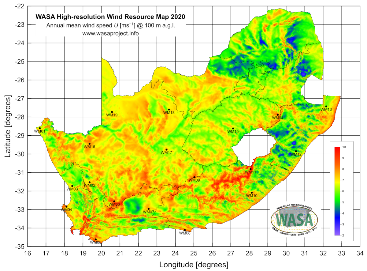
At latitude 28.601882, longitude 16.664410, and elevation 152 , the first station with Mast ID WM01 is located in Alexander Bay, a desert region of the Northern Cape. A second station is located in Humansdorp in the Eastern Cape with Mast ID WM08, longitude 24.514360, latitude 34.109965, and elevation 110 (also see Figure 2). A third station with Mast ID WM13 is located in the Jozini region of KwaZulu-Natal at longitude 32.16636, latitude 27.42605, and elevation 80 (see Table 3). Each of the data points of each station consists of 10 min averaged wind speed with varying features depending on the location (see Table 3).

Figure 2.
WASA high-resolution wind resource map (https://wasadata.csir.co.za/wasa1/WASAData) (accessed on 20 September 2022/5 June 2023).
Table 3.
Location description for the stations.
2.7. Performance Evaluation
2.7.1. Deterministic Forecast Evaluation Scores
For proper evaluation, robust and reliable models must be distinguished from weak ones using appropriate error metrics. Hence, we tested the accuracy of the prediction model in wind speed point forecasting using the RMSE, MAE, and MAPE, respectively, given by the following equations:
where is the error term; and and , respectively, denote the actual and predicted wind speed value. Smaller values of RMSE, MAE, and MAPE indicate a better predictive model. The penalisation of large errors by RMSE makes it susceptible to outliers. MAE is less sensitive to outliers but only considers errors’ magnitude, not their direction. Despite its scale dependence, MAPE overemphasises small errors when comparing models (see [9,42] for details). We also use the coefficient of determination or which is given by the equation below:
where represents the mean wind speed value. A better-fitted and preferred predictive model has an value much closer to 1. This indicator is highly sensitive to outliers.
2.7.2. Probabilistic Forecast Evaluation Scores
Probabilistic forecasting scores focus on assessing the model’s spread by taking into account the deviance of the conditional mean distribution to observed values. In this study, we tested the strength of the models in probabilistic forecasting through the PL function. Apart from its ability to deal with non-symmetric errors, the PL can be used to assess the reliability of interval predictions. The PL is given by [42]
where is the target quantile (i.e., ), the actual wind speed value, the quantile forecast The lower the PL value, the more accurate the quantile forecast.
We also used the DS score to evaluate the accuracy, sharpness, and reliability of probabilistic predictions. In this scoring rule, which only considers the mean and variance of a forecast distribution, broad distributions were penalised, whilst narrower distributions were incentivised, emphasising distribution sharpness. The DS is calculated by the following equation [43]:
where is the actual wind speed observation, denotes the mean and is the standard deviation of the forecast distribution. Lower values of the DS score imply more accurate and reliable probabilistic forecasts.
PIT histograms or values are used to evaluate the consistency between probabilistic forecasts and actual wind speed values. In an ideal forecast distribution, there would be no bins with extremely high or low levels on the PIT histogram. The PIT is computed using the equation below [44,45]:
where is the transformed variable and is the forecast distribution evaluated at the actual wind speed value . By transforming observed values into uniform distributions, the agreement between forecasts and actual data can then be examined. Smaller and uniformly distributed PIT values imply well-calibrated probabilistic forecasts; otherwise, the models’ probabilistic forecasts are miscalibrated or skewed.
2.7.3. Biasedness Assessment
Consider the residual terms denoted ,, if , then the model is either overestimating () or underestimating () the actual wind speed observation and is said to be biased. The MZ test regression function is given by the following equation (see [46] for details):
The MZ test evaluates the unbiasedness and consistency of the predictions, by testing the null hypothesis that the intercept () and slope () terms are respectively and . If parameter and , it indicates that the model’s predictions are unbiased and the prediction errors are minimal, otherwise, the model is considered biased. In essence, the rejection rule is such that if the p-value then the model is unbiased; otherwise the model is biased.
2.7.4. Predictive Accuracy Assessment
The MD was proposed by [47], and it graphically plots to compare the predictive strength of the models. Thus, MD displays forecast skill over various scoring functions, thereby enhancing comprehensive comparison and assessment of probabilistic model accuracy. Considering the loss function , the work of [47] showed that any consistent scoring function can be written in the following form:
where denotes a non-negative measure and
where . For events point forecasts, the average, denoted by can be calculated using the following mathematical expression:
3. Results
3.1. Computational Tools
We developed and executed comprehensive tests across all models within the Dell Intel Core i7 notebook development environment, utilising the R programming language. To accommodate the DE algorithm, we employed the “DEoptim” library, while the “wavelism” and ”wavelets” libraries were utilised for the selection of appropriate wavelet filters, including “d4”, “mb8”, and “la8” (see [48]). The “modwt” function from the “waveslim” library was instrumental in decomposing wind speed data sets into various sub-signals with varying frequency components. The GRU model was established and subsequently fitted using the “keras” library, a Python package (version 3.12) (see [49]). A systematic approach involving metaheuristic, early stopping and dropout regularisation was employed to identify the best hyperparameters for the models. The resulting best range of parameters is outlined in Table 4.
Table 4.
Model hyperparameters.
3.2. Exploratory Data Analysis
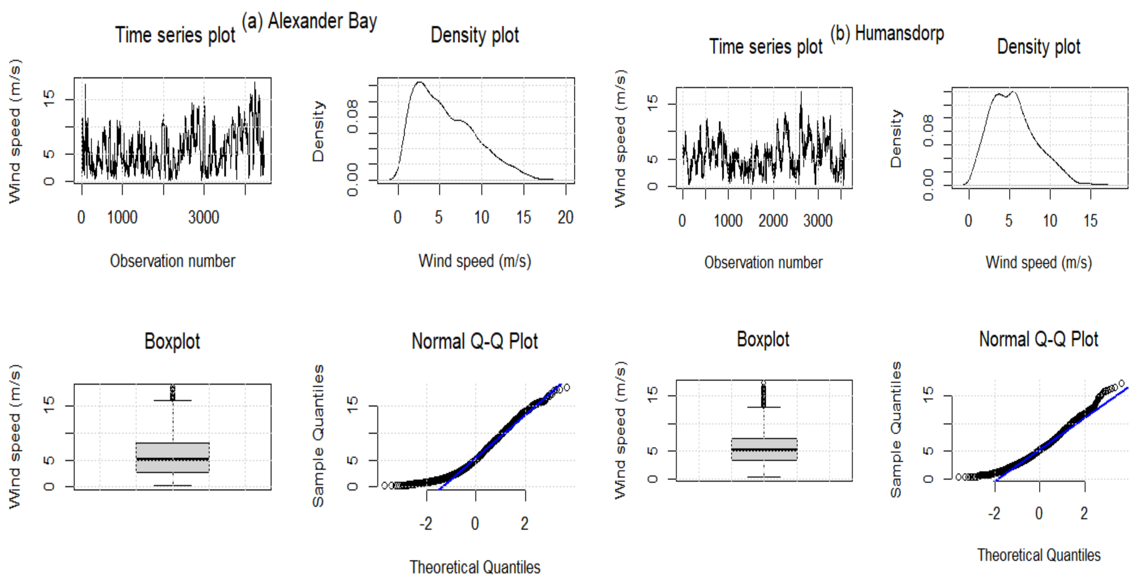
Table 5 summarises the descriptive statistics for wind speed data for the three WASA stations under investigation. The skewness values for all three stations are positive, indicating that wind data from each station has a positively skewed distribution (see Figure 3). In addition, the Jarque–Bera (JB) test (all p-values ) indicates that the three datasets are non-normal. This is also evident from the skewed density plots; the datasets under investigation have non-constant variance over time, illustrating some elements of cyclostationary patterns. In terms of standard deviation, Alexander Bay data seem more variant or volatile than other stations. Furthermore, data from Alexander Bay and Jozini stations are platykurtic since their kurtosis is less than 3. In the case of Humansdorp wind data, the kurtosis value is higher than 3, and the distribution is leptokurtic.
Table 5.
Descriptive statistics for wind speed data (in m/s) at the three stations of interest.
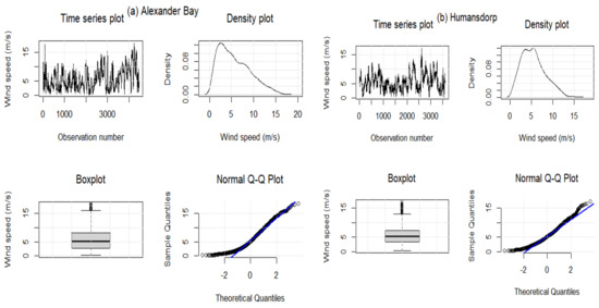

Figure 3.
Wind speed data for Alexander Bay (a), Humansdrop (b), and Jozini (c). Lines in blue represent QQ lines and boxes in grey indicate interquartile ranges.
3.3. Deterministic and Probabilistic Performance Evaluation
A summary of the results of point prediction accuracy indicators for the models explored at the three WASA stations, namely; Alexander Bay, Humansdorp, and Jozini, is presented in Table 6. The rationale is to assess the impact and effect of wavelet filters, decomposition level, location of the station, and forecasting scale/horizon on the proposed methods at both point and probabilistic forecasting levels. To effectively justify the predictive strength of the optimised and proposed decomposition level (), additional levels ( and ) were set out to do the same task using the wavelet-MODWT-GRU hybrid model. Additionally, three wavelet filters were used, namely; LA with eight (8) vanishing moments (i.e., “la8”) (denoted by M1), MB with eight (8) vanishing moments (i.e., “mb8”) (denoted by M3), and DB (denoted by M2) with four (4) vanishing moments (i.e., “d4“) for effective comparison. Besides, we also tested the efficacy of the best wavelet-MODWT-GRU among the wavelet filters against the individual GRU and benchmark naïve model. Best models are bolded.
Table 6.
Predictive performance indicators for the three wavelet filter models.
For the high-variant Alexander Bay dataset, model M3 optimised at produced the best results based on the least RMSE, MAE, MAPE, and highest values. Considering the MZ test, M1 was unbiased at and ; whilst M3 was unbiased at . Model M1 (), produced the second-best result based on the same indicators. The least desirable results were observed for M2 (). Overall, predictive accuracy is greatest at and declines as the decomposition level increases.
For the Humansdorp dataset, model M3 outcompeted all models at decomposition levels and based on the smallest RMSE, MAE, and the highest . As was observed in the Alexander Bay dataset, the optimised decomposition level () produced the best results in comparison with and ; and models’ strength seems to decrease with increasing decomposition levels. In terms of the MZ test, all models are unbiased across all decomposition levels, with the exception of M2 which is biased for . In general, the performance of M3 at a decomposition level was the best for the Humansdorp dataset.
For the least-variant Jozini dataset, model M3 () displayed the best performance as compared to other models and decomposition levels ( and). In fact, model M3 dominated all other models at decomposition levels and based on highest value of and the smallest values of MAE and MAPE. The MZ test showed that predictions from all models were unbiased (see Figure 4).
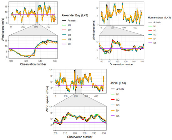
Figure 4.
Comparison of wind speed predictions against actual wind speed data for Alexander Bay (left panel), Humansdrop (right panel), and Jozini (bottom centre panel).
The comparative analysis showed that the performance of the models varied with the location of the station, wavelet filter applied, decomposition level, and the forecasting horizon. Overall, models seem to be more accurate and sharper on lower forecast horizons than on longer forecast horizons. For instance, the highest RMSE = 1.3119 value was recorded by M2 () at Alexander Bay station with forecast horizon , whilst the smallest RMSE was observed by model M3 () (RMSE = 0.4678 ) at Humansdorp station with . Similar to the work of [50], wavelet decomposition at higher levels produces more statistically sound sub-signals, but also produces larger error accumulations.
Table 7 compares the predictive performance of the best wavelet filter model (at ) with that of M4 (GRU) and benchmark M5 (naive). Using the skilled scores, we computed the predictive accuracy improvement relative to the benchmark M5 (see [42] for details). In essence, the skilled indicator produces a percentage that other models (i.e., M3 and M4) improve the benchmark model or M5. Our optimised proposed strategy dominated both the M4 and M5 models based on the smallest values of RMSE and MAE across the three datasets (also see Figure 4). In addition, the proposed hybrids produced the best results for the Humansdorp and Jozini datasets based on their lowest MAPE, whilst M4 produced the best results for the other station based on the same indicator. On the basis of the MZ test, the predictions from the proposed model (M3) were unbiased for Humansdorp and Jozini stations, whilst the predictions from model M5 were biased across all three datasets. In general, point error metrics indicated that model M3 provided the best predictions of wind speed data across the three stations.
Table 7.
Point performance indicators for the best wavelet filters model (at ) against the GRU and naïve model.
Table 8 presents the comparative evaluation of models using distributional forecast accuracy measures (i.e., PL, DS, and PIT). We used the PL and DS scores to measure model accuracy and uncertainty of predictions, whilst the PIT scores were used to assess models’ quality based on calibration. The smaller the values of PL, DS, and PIT, the better the probabilistic forecasts. Additionally, the model characterised by an unbiasedness model should have a uniform PIT histogram.
Table 8.
Distributional forecast accuracy indicators for the best wavelet filter model (at ) against the naïve (M5) and GRU (M4) model.
Model M4 produced the least values of PL for the Jozini and Alexander Bay datasets, whilst M5 produced the smallest PL value for the Humansdorp dataset. Based on the DS score, M3 outcompeted M4 and M5 with the lowest scores for the Alexander Bay, Humansdorp, and Jozini datasets. The DS Score indicator further showed that M4 produced the second-best results and demonstrated superiority over our benchmark for the Alexander Bay and Jozini datasets. Overall, model M3 had the most accurate and reliable predictions across the three datasets.
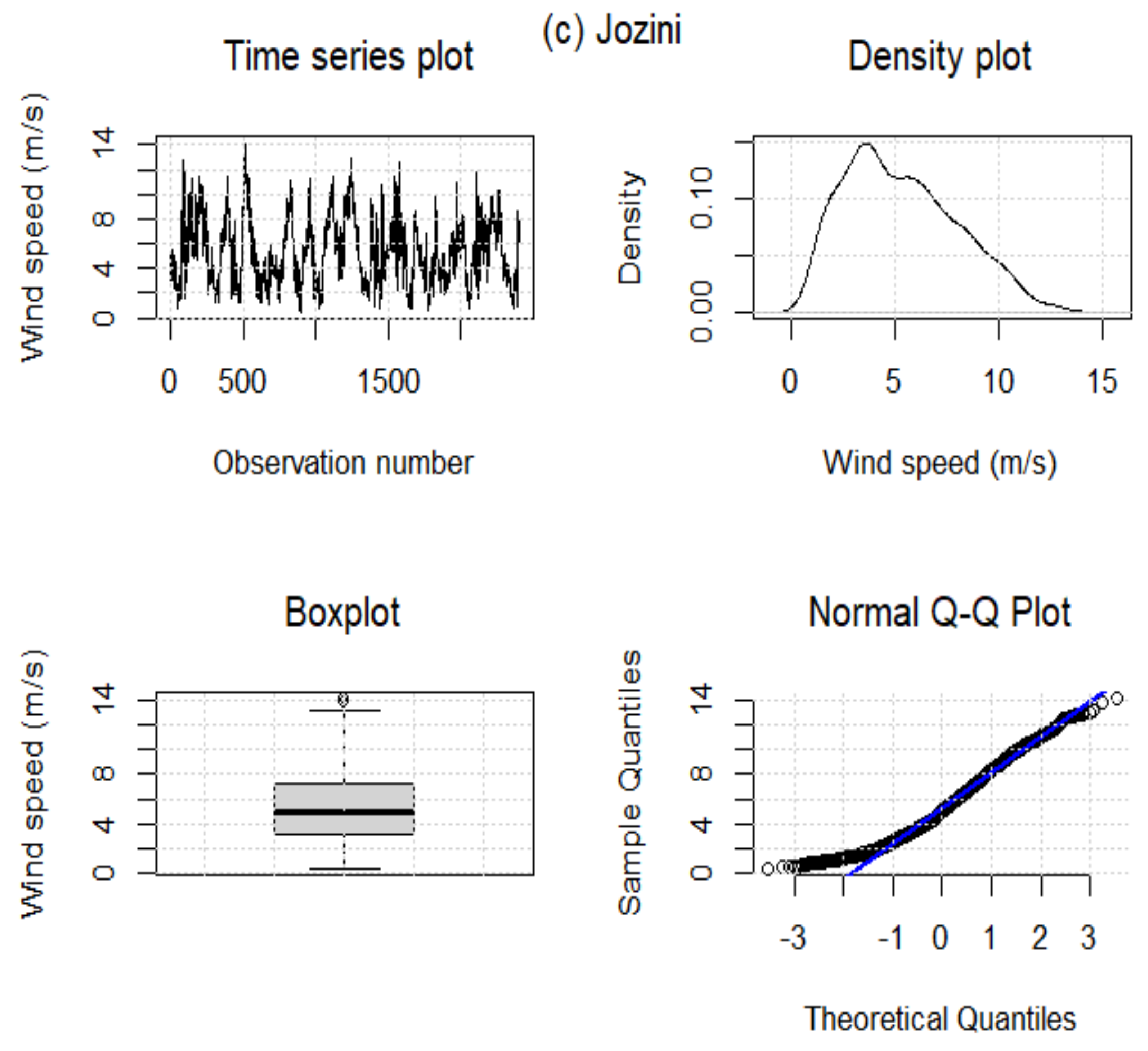
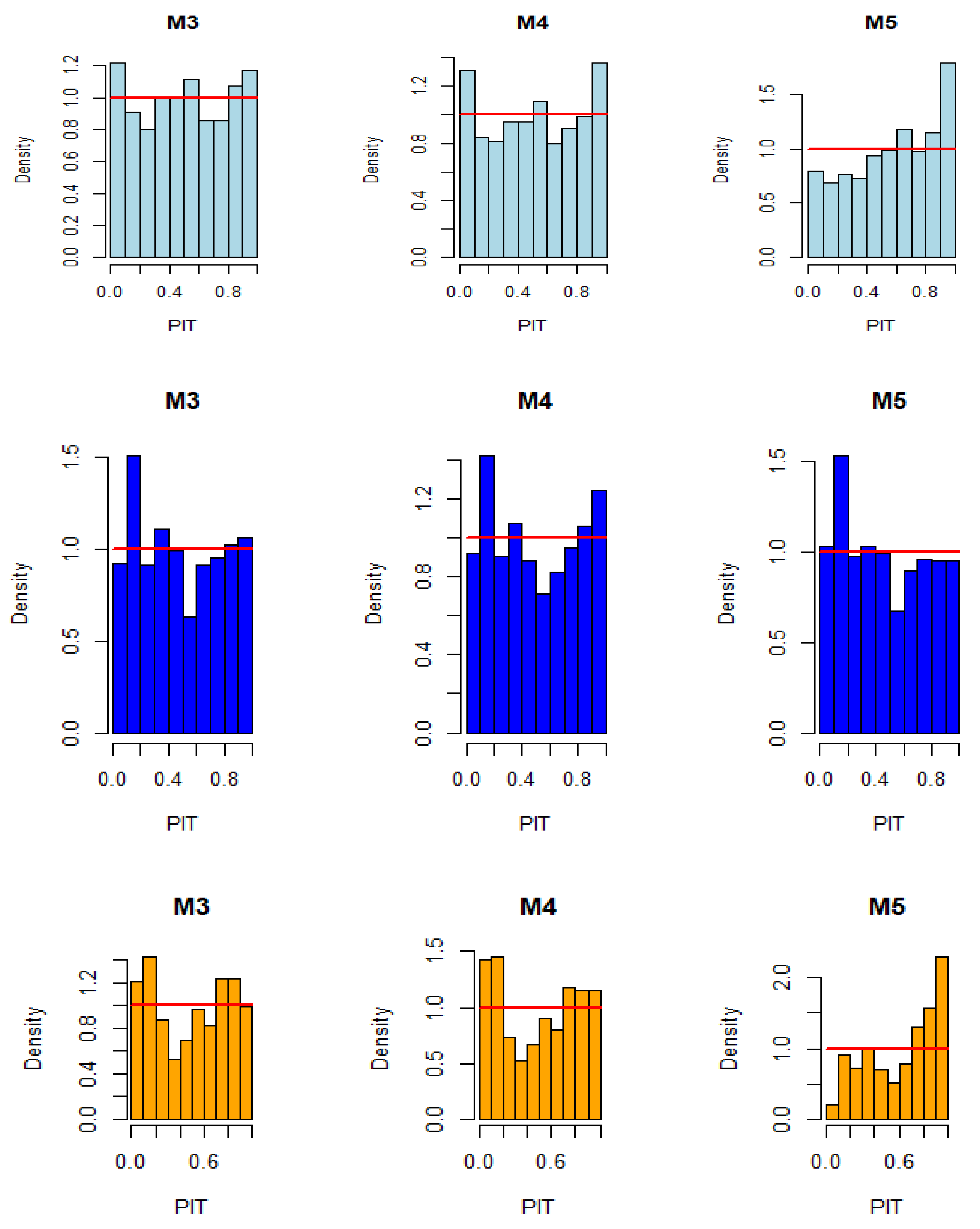
The PIT test statistics show that the proposed hybrid approach (i.e., M3) outcompeted both M4 and M5 for Alexander Bay and Jozini datasets by producing the smallest deviance between the observed and expected values. Furthermore, the Kolmogorov-Smirnov (KS) test showed that the p-values for M3 are greater than 0.05 for the Alexander Bay and Humansdorp datasets. Thus, we do not reject the null hypothesis that the PIT values are uniformly distributed. Hence, the predictions from these models are well-calibrated and unbiased for the respective datasets. Although the p-value at the Jozini data station, M3 outcompeted both M4 and M5 in producing the least biased and deviant predictions that are better-calibrated (see Figure 5).

Figure 5.
PIT Histograms for the Alexander Bay (top panel), Humansdorp (middle panel), and Jozini (bottom panel) comparing models M3, M4, and M5.
Overall, M3 produced the most accurate, reliable, and well-calibrated predictions for the Alexander Bay, Humansdorp, and Jozini datasets. Across all datasets, preprocessed models through WT at the optimised decomposition level () were superior in terms of prediction accuracy, reliability, and calibration over those that have not been preprocessed.
3.4. Predictive Performance Analysis
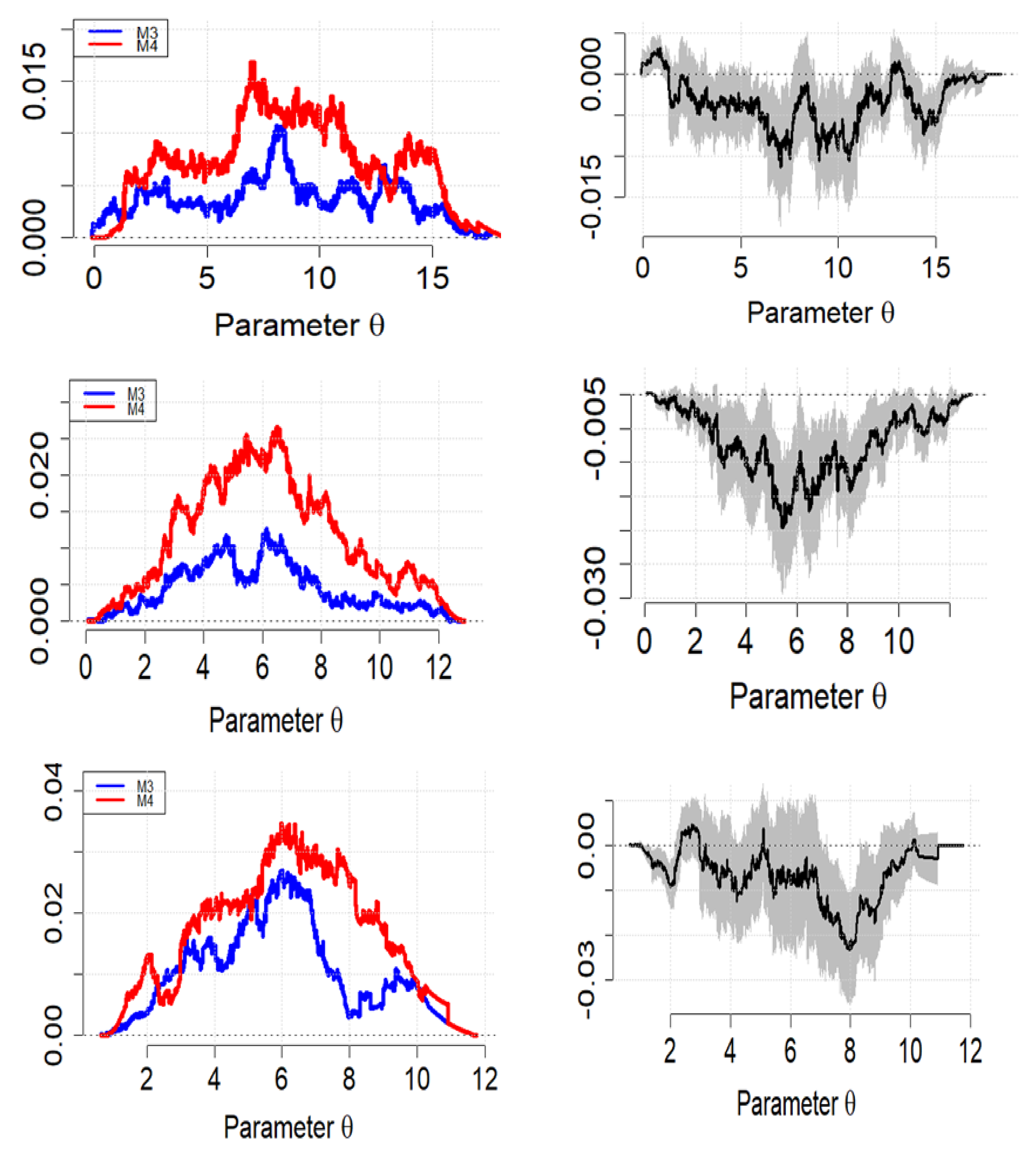
The MDs are provided in Figure 6 for comparing the predictive accuracy of our proposed strategy against model M4 (or GRU). For Alexander Bay data (top panel), model M3 showed clear dominance (blue curve mostly below the red curve) over model M4, as illustrated in the top panel of Figure 6. A slight curve overlap at the extreme values was also observed. In addition, empirical score differences are mostly negative values, with a slightly wider and broader range of 95% prediction interval scores.
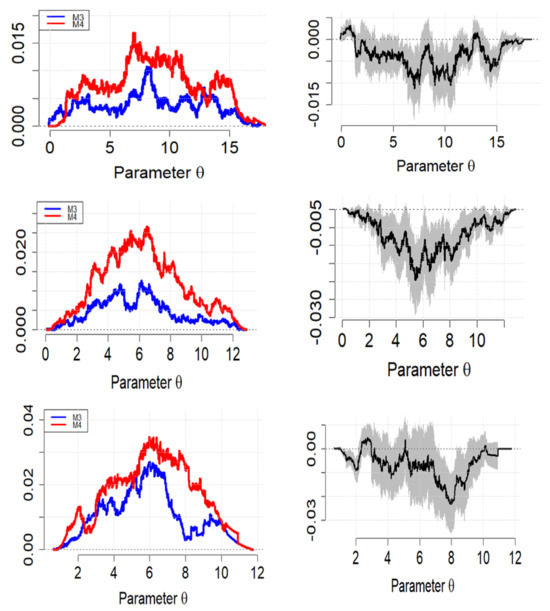
Figure 6.
Murphy diagrams with 95% confidence intervals: M3 and M4 (upper panel, Alexander Bay), (centre panel, Humansdorp), and (bottom panel, Jozini). Shaded regions indicates 95% confidence intervals for the difference between the two functions.
The empirical score curve in Figure 6 (middle panel) shows that M3 dominated M4 for the Humansdorp data. For this data station, M3 provided better prediction accuracy than M4. Furthermore, the difference in scores with a majority of negative ratings had a wider (but slightly broader as compared to Alexander Bay data) 95% prediction interval.
The MD results for the Jozini data (bottom panel of Figure 6) show that M3 had superior predictive power than M4. Furthermore, the empirical score differences were mostly negative values with a slightly wider range of 95% prediction intervals when compared to the other two datasets. Similar to the Alexander Bay, curves overlapping the extreme values were also observed.
Overall, the MD confirms the results deduced from the other performance indicators, and it indicates that model M3 provides the best forecasts for all three datasets. Furthermore, the 95% interval range width seems much narrower for high-variant data and a longer forecasting horizon.
Table 9 compares the forecasting performance of the proposed approach (M3) compared to that of M4 and M5 at different lead time intervals based on the high-variant Alexander Bay dataset. Ideally, we would like to assess the accuracy, generalisability, and robustness of the proposed approach as lead time increases from 10 min to 60 min (or 1 h). As evidenced by the increases in the values of error metrics (except MAPE for model M3) and reductions in the skill score values, it can be deduced from Table 9 that the models forecasting performance reduces with increases in lead times. Nonetheless, the proposed approach (M3) still demonstrates clear dominance and superiority in predictive forecasting over all other models even at a 1 h lead time.
Table 9.
Effect of the lead times on model performance using the Alexander Bay dataset (at ).
4. Conclusions
While wind power has numerous advantages, one of the most challenging aspects of integrating large volumes of wind power into an existing electrical power grid is that wind resource (i.e., wind speed) has inherent climatic behaviour, characterised by high intermittent and continuous variations in its intensity. This type of behaviour often encompasses aspects of both linearity and nonlinearity. Attempting to characterise it using a single model (let alone a linear model) is impractical and potentially erratic, ultimately impacting wind power investment decisions.
The study proposes a hybrid strategy that integrates MODWT wavelet filters, DE algorithms, and GRUs for wind speed forecasting, referred to as wavelet-MODWT-GRUs. This approach was tested using high-resolution wind data averaged over 10 min from WASA data stations located in Alexander Bay, Humansdorp, and Jozini, South Africa. We began with a comparative analysis of the wavelet-MODWT-GRUs employing LA8, DB4, and MB8 filters across various decomposition levels (i.e., , and ). The efficacy of the best wavelet-MODWT-GRU at each of the three stations was subsequently validated and compared with the individual GRU, while also being benchmarked against the naïve model.
The point forecast error indicators (i.e., RMSE, MAE, and MAPE) and showed that the proposed models’ predictive performance at the decomposition level optimised through DE was best across all three datasets and wavelet filters. The filter-wise comparative analysis further revealed that the MB-MODWT-GRU at produced the most accurate and unbiased wind speed predictions for the Alexander Bay data, Humansdorp, and Jozini datasets.
In probabilistic forecasting, the DS and PIT scores also showed that the MB-MOWT-GRU dominated GRU and the naïve model in terms of the most reliable and calibrated probabilistic forecasts across the three datasets. MD diagram analysis shows that MB-MODWT-GRU models dominated the GRU and naive models across all three datasets. From the comparative analysis, we can conclude the following:
- DE optimises the decomposition level (at ) efficiently and simply, resulting in MODWT decomposed sub-signals that are easier to characterise for GRU modelling.
- The location of the station, wavelet filter applied, decomposition level, and forecasting horizon all affected model performance.
- The MB filter (followed by the LA filter) produced better wind speed forecasts for short-to-longer forecast horizons, less variant-to-high-variant, and small-to-larger datasets.
- The prediction error tends to increase as the decomposition level increases. Similar results were obtained in [20,50].
- The application of MODWT reduces noise and volatility in wind speed data, thereby improving the prediction performance of all hybrids. Consequently, complex wind speed data sub-signals were accurately and reliably captured via the GRU model. These results concur with the work of [4,19].
- Although the naive model is easy to understand, it is ineffective when dealing with wind speed data. Similar results were obtained in the work of [10].
- Generally, the increase in lead times led to an increase in error metrics and a decrease in the predictive ability of all models. Nonetheless, the proposed approach still demonstrated superiority over all other models.
The proposed strategy will enable utility managers to integrate wind energy into power grids while developing a deeper knowledge of MODWT-based hybrids and wind speed measurements. However, only three wavelet filters were examined in the current study, which used small South African wind speed data. There is potential for future research to utilise larger and more complex datasets from varying regions within and outside the country with other wavelet filters (e.g., Meyer, Morlert, etc.). Moreover, the proposed strategy can be improved further by using other effective and data-efficient optimisation strategies, such as Bayesian optimisation (infused with cross-validation) and GRU. Future work will also look at spatially aggregating wind speed forecasting from multiple wind farms to diversify variability.
Author Contributions
Conceptualisation, K.S.S.; methodology, K.S.S.; software, K.S.S.; validation, K.S.S. and E.R.; formal analysis, K.S.S.; investigation, K.S.S.; resources, K.S.S. and E.R.; data curation, K.S.S.; writing-original draft, K.S.S.; writing review and editing, K.S.S. and E.R.; visualisation, K.S.S.; supervision, E.R. All authors have read and agreed to the published version of the manuscript.
Funding
This research received no external funding.
Institutional Review Board Statement
Not applicable.
Informed Consent Statement
Not applicable.
Data Availability Statement
These wind speed data can be downloaded from the WASA website (https://wasadata.csir.co.za/wasa1/WASAData) (accessed 20 September 2022/5 June 2023).
Conflicts of Interest
The corresponding author states that there are no conflicts of interest.
References
- Zhen, H.; Niu, D.; Yu, M.; Wang, K.; Liang, Y.; Xu, X. A Hybrid Deep Learning Model and Comparison for Wind Power Forecasting Considering Temporal-Spatial Feature Extraction. Sustainability 2020, 12, 9490. [Google Scholar] [CrossRef]
- Wang, X.; Guo, P.; Huang, X. A Review of Wind Power Forecasting Models. Energy Procedia 2011, 12, 770–777. [Google Scholar] [CrossRef]
- Chandra, D.; Sailaja Kumari, M.; Sydulu, M.; Grimaccia, F.; Mussetta, M. Adaptive Wavelet Neural Network-Based Wind Speed Forecasting Studies. J. Electr. Eng. Technol. 2014, 9, 1812–1821. [Google Scholar] [CrossRef]
- Sivhugwana, K.S.; Ranganai, E. An Ensemble Approach to Short-Term Wind Speed Predictions Using Stochastic Methods, Wavelets and Gradient Boosting Decision Trees. Wind 2024, 4, 44–67. [Google Scholar] [CrossRef]
- Soman, S.S.; Zareipour, H. A Review of Wind Power and Wind Speed Forecasting Methods with Different Time Horizons. In Proceedings of the North American Power Symposium 2010, Arlington, TX, USA, 26–28 September 2010. [Google Scholar] [CrossRef]
- Gardner, W.A.; Napolitano, A.; Paura, L. Cyclostationarity: Half a Century of Research. Signal Process. 2006, 86, 639–697. [Google Scholar] [CrossRef]
- Percival, D.B.; Walden, A.T. Wavelet Methods for Time Series Analysis; Cambridge University Press: Cambridge, UK, 2000. [Google Scholar]
- Zhang, Z.; Telesford, Q.K.; Giusti, C.; Lim, K.O.; Bassett, D.S. Choosing Wavelet Methods, Filters, and Lengths for Functional Brain Network Construction. PLoS ONE 2016, 11, e0157243. [Google Scholar] [CrossRef]
- Gensler, A. Wind Power Ensemble Forecasting: Performance Measures and Ensemble Architectures for Deterministic and Probabilistic Forecasts. Ph.D. Thesis, University of Kassel, Hessen, Germany, 21 September 2018. [Google Scholar]
- Singh, S.N.; Mohapatra, A. Repeated Wavelet Transform-Based ARIMA Model for Very Short-Term Wind Speed Forecasting. Renew. Energy 2019, 136, 128. [Google Scholar] [CrossRef]
- Valdivia-Bautista, S.M.; Domínguez-Navarro, J.A.; Pérez-Cisneros, M.; Vega-Gómez, C.J.; Castillo-Téllez, B. Artificial Intelligence in Wind Speed Forecasting: A Review. Energies 2023, 16, 2457. [Google Scholar] [CrossRef]
- Catalão, J.P.S.; Pousinho, H.M.I.; Mendes, V.M.F. Short-Term Wind Power Forecasting in Portugal by Neural Networks and Wavelet Transform. Renew. Energy 2011, 36, 1245–1251. [Google Scholar] [CrossRef]
- Berrezzek, F.; Khelil, K.; Bouadjila, T. Efficient Wind Speed Forecasting Using Discrete Wavelet Transform and Artificial Neural Networks. Rev. d’Intelligence Artificielle 2019, 33, 447–452. [Google Scholar] [CrossRef]
- Niu, D.; Pu, D.; Dai, S. Ultra-Short-Term Wind-Power Forecasting Based on the Weighted Random Forest Optimized by the Niche Immune Lion Algorithm. Energies 2018, 11, 1098. [Google Scholar] [CrossRef]
- Patel, Y.; Deb, D. Machine Intelligent Hybrid Methods Based on Kalman Filter and Wavelet Transform for Short-Term Wind Speed Prediction. Wind 2022, 2, 37–50. [Google Scholar] [CrossRef]
- Catalão, J.P.S.; Pousinho, H.M.I.; Mendes, V.M.F. Hybrid Wavelet-PSO-ANFIS Approach for Short-Term Wind Power Forecasting in Portugal. IEEE Trans. Sustain. Energy 2011, 2, 50–59. [Google Scholar] [CrossRef]
- Xiang, J.; Qiu, Z.; Hao, Q.; Cao, H. Multi-Time Scale Wind Speed Prediction Based on WT-Bi-LSTM. MATEC Web Conf. 2020, 309, 05011. [Google Scholar] [CrossRef]
- Liu, Y.; Guan, L.; Hou, C.; Han, H.; Liu, Z.; Sun, Y.; Zheng, M. Wind Power Short-Term Prediction Based on LSTM and Discrete Wavelet Transform. Appl. Sci. 2019, 9, 1108. [Google Scholar] [CrossRef]
- Sivhugwana, K.S.; Ranganai, E. Short-Term Wind Speed Prediction via Sample Entropy: A Hybridisation Approach against Gradient Disappearance and Explosion. Computation 2024, 12, 163. [Google Scholar] [CrossRef]
- Domínguez-Navarro, J.A.; Lopez-Garcia, T.B.; Valdivia-Bautista, S.M. Applying Wavelet Filters in Wind Forecasting Methods. Energies 2021, 14, 3181. [Google Scholar] [CrossRef]
- Khelil, K.; Berrezzek, F.; Bouadjila, T. GA-based design of optimal discrete wavelet filters for efficient wind speed forecasting. Neural Comput. Appl. 2020, 33, 4373–4386. [Google Scholar] [CrossRef]
- Morris, J.M.; Peravali, R. Minimum-bandwidth discrete-time wavelets. Signal Process. 1999, 76, 181–193. [Google Scholar] [CrossRef]
- Storn, R.; Price, K. Differential evolution–a simple and efficient heuristic for global optimization over continuous spaces. J. Glob. Optim. 1997, 11, 341–359. [Google Scholar] [CrossRef]
- Wang, Y.; Cai, Z.; Zhang, Q. Differential Evolution With Composite Trial Vector Generation Strategies and Control Parameters. IEEE Trans. Evol. Comput. 2011, 15, 55–66. [Google Scholar] [CrossRef]
- Eltaeib, T.; Mahmood, A. Differential Evolution: A Survey and Analysis. Appl. Sci. 2018, 8, 1945. [Google Scholar] [CrossRef]
- Leon, M.; Xiong, N. Investigation of Mutation Strategies in Differential Evolution for Solving Global Optimization Problems. In Artificial Intelligence and Soft Computing, ICAISC 2014; Rutkowski, L., Korytkowski, M., Scherer, R., Tadeusiewicz, R., Zadeh, L.A., Zurada, J.M., Eds.; Lecture Notes in Computer Science, 8467; Springer: Cham, Switzerland, 2014. [Google Scholar] [CrossRef]
- Merry, R.J.E. Wavelet Theory and Applications: A Literature Study; DCT Rapporten; Technische Universiteit Eindhoven: Eindhoven, The Netherlands, 2005. [Google Scholar]
- Daubechies, I. Ten Lectures on Wavelets; Society for Industrial and Applied Mathematics: Philadelphia, PA, USA, 1992. [Google Scholar]
- Gröchenig, K. Foundations of Time-Frequency Analysis; Springer Science & Business Media: New York, NY, USA, 2001. [Google Scholar]
- Kovačević, J.; Goyal, V.K. Fourier and Wavelet Signal Processing; Verlag Nicht Ermittelbar: 2010. Available online: https://www.fourierandwavelets.org/FWSP_a3.2_2013.pdf (accessed on 4 October 2024).
- Mallat, S.G. A Theory for Multiresolution Signal Decomposition: The Wavelet Representation. IEEE Trans. Pattern Anal. Mach. Intell. 1989, 11, 674–693. [Google Scholar] [CrossRef]
- Misiti, M.; Misiti, Y.; Oppenheim, G.; Poggi, J.M. Wavelets Toolbox User’s Guide; The MathWorks: Natick, MA, USA, 2000. [Google Scholar]
- Dghais, A.A.; Ismail, M.T. A Comparative Study between Discrete Wavelet Transform and Maximal Overlap Discrete Wavelet Transform for Testing Stationarity. Int. J. Math. Comput. Phys. Electr. Comput. Eng. 2013, 7, 1677–1681. [Google Scholar]
- Rodrigues, D.V.Q.; Zuo, D.; Li, C. A MODWT-Based Algorithm for the Identification and Removal of Jumps/Short-Term Distortions in Displacement Measurements Used for Structural Health Monitoring. IoT 2022, 3, 60–72. [Google Scholar] [CrossRef]
- Alarcon-Aquino, V.; Barria, J.A. Change Detection in Time Series Using the Maximal Overlap Discrete Wavelet Transform. Lat. Am. Appl. Res. 2009, 39, 145–152. [Google Scholar]
- Zaharie, D. A Comparative Analysis of Crossover Variants in Differential Evolution. In Proceedings of the International Multiconference on Computer Science and Information Technology, Gosier, Guadaloupe, 4–9 March 2007; pp. 171–181. Available online: https://staff.fmi.uvt.ro/~daniela.zaharie/lucrari/imcsit07.pdf (accessed on 2 October 2024).
- Eiben, Á.E.; Hinterding, R.; Michalewicz, Z. Parameter Control in Evolutionary Algorithms. IEEE Trans. Evol. Comput. 1999, 3, 124–141. [Google Scholar] [CrossRef]
- Mullen, K.M.; Ardia, D.; Gil, D.L.; Windover, D.; Cline, J. DEoptim: An R package for global optimization by differential evolution. J. Stat. Softw. 2011, 40, 1–26. [Google Scholar] [CrossRef]
- Hochreiter, S.; Schmidhuber, J. Long Short-Term Memory. Neural Comput. 1997, 9, 1735–1780. [Google Scholar] [CrossRef]
- Cho, K.; van Merrienboer, B.; Bahdanau, D.; Bengio, Y. On the Properties of Neural Machine Translation: Encoder-Decoder Approaches. arXiv 2014, arXiv:1409.1259. [Google Scholar] [CrossRef]
- Chung, J.; Gulcehre, C.; Cho, K.; Bengio, Y. Empirical Evaluation of Gated Recurrent Neural Networks on Sequence Modeling. arXiv 2014, arXiv:1412.3555. [Google Scholar] [CrossRef]
- Hyndman, R.J.; Athanasopoulos, G. Forecasting: Principles and Practice, 2nd ed.; OTexts: Melbourne, Australia, 2021. [Google Scholar]
- Jordan, A.; Krüger, F.; Lerch, S. Evaluating probabilistic forecasts with scoringRules. J. Stat. Softw. 2019, 90, 1–37. Available online: https://www.jstatsoft.org/article/view/v090i12 (accessed on 17 December 2024). [CrossRef]
- Gneiting, T.; Raftery, A.E. Strictly Proper Scoring Rules, Prediction, and Estimation. J. Am. Stat. Assoc. 2007, 102, 359–378. [Google Scholar] [CrossRef]
- Bosse, N.I.; Gruson, H.; Cori, A.; van Leeuwen, E.; Funk, S.; Abbott, S. Evaluating Forecasts with Scoringutils in R. arXiv 2022, arXiv:2205.07090. [Google Scholar] [CrossRef]
- Mincer, J.; Zarnowitz, V. The Evaluation of Economic Forecasts. In Economic Forecasts and Expectations; National Bureau of Economic Research: Cambridge, MA, USA, 1969; pp. 3–46. Available online: https://www.nber.org/system/files/chapters/c1214/c1214.pdf (accessed on 17 June 2024).
- Werner, E.; Tilmann, G.; Alexander, J.; Fabian, K. Of Quantiles and Expectiles: Consistent Scoring Functions, Choquet Representations, and Forecast Rankings. J. R. Stat. Soc. B 2016, 78, 505–562. [Google Scholar] [CrossRef]
- Whitcher, B. waveslim: Basic Wavelet Routines for One-, Two-, and Three-Dimensional Signal Processing; R package version 1.8.5; 2024. Available online: https://cran.r-project.org/package=waveslim (accessed on 3 October 2024).
- Allaire, J.J.; Chollet, F. Keras: R Interface to ‘Keras’. CRAN: Contributed Packages. R Package. 2024. Available online: https://cran.r-project.org/web/packages/keras/vignettes/ (accessed on 21 June 2024).
- Kaur, D.; Lie, T.T.; Nair, N.K.; Vallès, B. Wind Speed Forecasting Using Hybrid Wavelet Transform-ARMA Techniques. Aims Energy 2015, 3, 13–24. [Google Scholar] [CrossRef]


Disclaimer/Publisher’s Note: The statements, opinions and data contained in all publications are solely those of the individual author(s) and contributor(s) and not of MDPI and/or the editor(s). MDPI and/or the editor(s) disclaim responsibility for any injury to people or property resulting from any ideas, methods, instructions or products referred to in the content. |
© 2025 by the authors. Licensee MDPI, Basel, Switzerland. This article is an open access article distributed under the terms and conditions of the Creative Commons Attribution (CC BY) license (https://creativecommons.org/licenses/by/4.0/).