Abstract
Assessment and evaluation of damage in cultural heritage structures are conducted primarily using nondestructive and noncontact methods. One common deployment is laser scanners or ground-based lidar scanners that produce a point cloud containing information at the centimeter to the millimeter level. This type of data allows for detecting surface damage, defects, cracks, and other anomalies based only on geometric surface descriptors using a single dataset, which does not rely on a change detection approach. Moreover, geometric features are not influenced by color, which is essential for heritage structures because they are nonuniform in color due to anthropologic and environmental effects (e.g., painting or moisture). In this work, a damage detection method developed based on local geometric features is evaluated and expanded for crack detection within the example fresco walls of Sala degli Elementi in the Palazzo Vecchio. The workflow’s performance is then compared in a qualitative manner to that of manual crack mapping results identified using images.
1. Introduction
Technologies to collect remotely sensed data based on active and passive data acquisition approaches have evolved in the last decade, enabling users to utilize these technologies for various applications. Within the field of engineering, remote sensing technologies are mainly used to create two-dimensional (2D) or three-dimensional (3D) representation of regions of interest (ROI) for applications such as capturing complex geometry of structures, scenes, or objects and structural health monitoring tasks, including deformation monitoring and damage detection and quantification at various level of detail (LODs) [1,2,3,4]. Among the available remote sensing platforms, ground-based light detection and ranging (lidar) platforms (also referred to as terrestrial lidar or laser scanner) are used as a nondestructive assessment technique to analyze the ROI at the member level. Ground-based lidar (GBL) platforms can collect highly detailed and geometrically accurate 3D representations of the ROI and may contain the true color and the intensity return values. GBL outputs a 3D point cloud, a set of points in 3D space representing objects’ surface. Due to the unstructured nature of the point clouds, these data representations are initially used for tasks such as measurement and visualizations. As a result, multiple methodologies have been introduced to process and analyze point clouds for damage detection by extracting and exploiting various features such as local geometric variations of points, color, or intensity value variation of the points, as well as comparing temporal datasets for change detection analysis [5,6,7,8,9].
This study aims to analyze the point cloud representation of the walls of a culturally prominent structure, namely Palazzo Vecchio, which is located in the city of Florence, Tuscany, Italy (Figure 1). Palazzo Vecchio is a historical building where many of the interior walls contain culturally important frescos (paintings with waterborne colors). The analyzed wall segment is located in a room at the southeast corner structure, known as Sala degli Elementi. The analyzed wall segment sustained significant cracking on its interior walls, where a single point cloud data of the wall segment is processed using an extension of the method introduced by Mohammadi et al. [9]. Single point cloud data here emphasizes that the analysis is performed without relying on comparison between two or more datasets collected at different times. The developed method relies on the local geometric variations that are not affected by color, which is essential for heritage structures due to color nonuniformities introduced by anthropologic and environmental effects. The damage detection and results using remote sensing point cloud data enable objective damage detection analysis, provide immediate guidance for in-person condition assessment, can be used as a baseline to monitor the damage and its progress. These are essential tools for heritage structure evaluations by providing insight into understanding the potential damage mechanisms and identifying potential rehabilitation. Lastly, it provides digital documentation of the scene in case of an emergency or unforeseen events to rehabilitate the damaged areas of cultural importance [10].
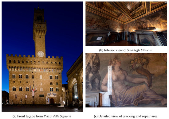
Figure 1.
Palazzo Vecchio’s structure as located in the city of Florence, Tuscany, Italy.
2. Background
Within the field of vision-based structural health monitoring, damage detection from point clouds has been investigated as a nondestructive assessment technique through multiple workflows. These workflows are developed based on pattern recognition, supervised or unsupervised machine learning, or change detection analysis approaches. Therefore, these studies can be classified into four broad groups based on the approach used to detect damaged areas discussed in this section. In addition to the approaches used to detect damaged areas, multiple studies use both active (i.e., lidar) and passive (i.e., imagery) remote sensing technologies to collect data from the damaged areas and further process these data to detect and quantify damaged areas and compare each technology. As one of the early studies, Olsen et al. collected lidar point clouds of a full-scale beam-column joint [2]. Within the study, the authors quantified the volumetric losses by adding the cross-sectional areas at multiple locations and studied the application of the GBL platform to perform crack mapping via collected colored images (i.e., color information) and intensity return values. However, as Olsen et al. reported, the crack mapping developed through color and intensity information was not able to represent the exact location of the cracks due to parallax [2]. Laefer et al. investigated the application of GBL and high-resolution photogrammetry to detect cracking and compared the results with a manual or visual inspection. To collect lidar data, the authors positioned the GBL platform at various distances, which resulted in point clouds with point-to-point distances of 1.00 to 1.75 mm within the ROI. The research concluded that lidar-derived point clouds with such point-to-point spacing were not reliable nor efficient data sources to detect cracking in comparison to digital images [11]. Laefer et al. further investigated the application of GBL-derived point clouds in detecting cracks by developing mathematical equations that characterize the minimum detectable crack widths based on orthogonal distance offset between GBL platform and ROI, interval scan angle, the crack orientation, and crack depth [12]. Based on the developed equations and the verification study, the authors have reported that the GBL-derived point clouds collected at a distance of fewer than 10.0 m can reliably detect the vertical cracks of at least 5 mm or larger. This was supported by the earlier study of Laefer et al. [11]. However, the authors observed that quantified crack widths were consistently overestimated. In addition, it is where the crack detection was performed using a semi-manual process. More recently, Chen et al. developed an experiment similar to that created by Laefer et al. in 2014 to evaluate the Structure-from-Motion (SfM)-derived point clouds [13]. Within this study, the authors varied the camera locations to study the effects of different angles and distances to ROI in the final SfM-derived point cloud. To compare the accuracy of the SfM-derived point cloud, five features were selected with the test specimen and then shifted, and the displacement of these features was measured and compared to the values computed from the lidar-derived point clouds. The authors reported that the SfM-derived point cloud that is created based on images collected at multiple distances and angles resulted in the most accurate measurements.
The studies that incorporate a pattern recognition approach are comprised of two main components. The first component of these workflows includes the feature extractors that analyze input data based on its properties and provide features useful for the classification of damaged and undamaged areas. The second component of these workflows is the classifier which analyzes the extracted features and assigns a label to the input instant. The main difference between pattern recognition and machine learning approaches is that the machine learning workflows employ feedback from the predicted labels to the classifier and, in some cases, to the feature extractors (e.g., convolutional neural network (CNN)) to develop the classifier. Several studies have used pattern recognition to detect damage from point clouds. For example, Torok et al. introduced a damage detection method based on a point cloud of a column with planar surfaces [14]. Within the introduced workflow, a mesh representation of the input point cloud was identified and transformed such that the vertical direction of the column is parallel with the global vertical direction. Within this study, the features were computed by calculating the angle between each mesh element normal vector and the selected reference normal vector. Torok et al. used a straightforward classifier to identify damaged regions, where a region is considered damaged if the corresponding calculated angle was within the predefined threshold limit. Kim et al. presented a method to detect and spalling damage of a flat concrete surface [15]. Like Torok et al., the proposed workflow used a variation of normal vectors with respect to a reference vector as one of the damage-sensitive features. However, the normal vectors were computed for each point through Principal Component Analysis (PCA) approach. In addition to normal vectors, Kim et al. used the variation of vertical distances between each point and best-fitted plane to the concrete block surface as the second damage-sensitive feature. Lastly, the classifier combined the result of each damage sensitive feature through an equation to identify the damaged areas. Valenca et al. presented a more advanced workflow to detect cracks on a concrete surface through combining detection results from 2D images in addition to computing the distance variation of points to a reference plane [16]. To detect damaged areas, the proposed method initially evaluated the distance variations to identify damaged areas based on point clouds. Then, image-based damage analysis results were supplemented with the results of distance variation to improve the damage detection accuracy. Erkal and Hajjar proposed workflow identified damage areas through various methods, including the variation of point normal vectors as well as supplementing normal vector based results with damage detection result based on color and/or intensity information [3]. Within this study, the damage detection results were based on normal vector followed a similar procedure to that of Kim et al. [15]. However, Erkal and Hajjar recommended three different options to determine the reference vector, which provides more flexibility than previous studies [3]. The damage identification using intensity or color information was conducted by classifying the points based on each point’s selected neighbors’ threshold value.
The next group of studies is developed based on the supervised machine learning approaches, where the input instances are associated with known labels. The main component in the machine learning-based workflows is to develop a classifier that learns the mapping from the input instances based on the extracted features to the output correctly by updating the learnable classifier parameters. The features within supervised machine learning approaches are identified based on engineered feature extractors or learned during developing the classifier (i.e., training) and the classifier. For example, Vetrivel et al. used SfM-derived point clouds and oblique aerial images to detect damaged areas using multiple kernels supervised learning approaches [17]. Within this study, Vetrivel et al. extracted features from point cloud instances through PCA and further analyze the features using CNN. In parallel, the corresponding image of 3D point cloud instances was analyzed by a support vector machine classifier to identify the damaged areas. This proposed workflow was developed and tested at the building level [18]. More recently, Nasrollahi et al. utilized a well-established deep learning network, PointNet [19], to detect cracks in a flat concrete block [20]. While the deep learning-based models eliminated the need to develop and design damage-sensitive features, these models’ success was tied to a large number of training instances. To train the classifier, Nasrollahi et al. normalized the coordinates and incorporated the color information to improve the detection results and concluded that the developed model could achieve a detection accuracy of 88%. More recently, Haurum et al. investigated the application of two well-established deep learning classifiers, namely Dynamic Graph CNN (DGCNN) [21] and PointNet [19], to detect damaged areas within synthetic point cloud datasets that simulate damage within sewer pipelines [22]. In this study, the point cloud instances were initially preprocessed to remove the erroneous points based on statistical outlier removal presented by Barnett and Lewis [23]. As the machine learning-based models required the input instances to have a consistent number of instances, the input instances were either downsampled or upsampled to meet this criterion. Haurum et al. labeled the points based on three types of defects predominantly observed within the sewer pipelines and reported that DGCNN could detect damaged labels with precision and recall accuracy of 60%.
A fourth group of studies is developed based on unsupervised learning algorithms. Contrary to supervised learning algorithms, the labels are not known in an unsupervised learning approach. Therefore, the unsupervised learning algorithm’s main component is identifying the criteria or regulations that categorize the input instances into separate groups or clusters. In these workflows, the spatial location of points, color information, and/or intensity return values of points are utilized directly as features or processed to provide a more robust set of discriminative features to classify points within the damaged areas. For example, Kashani and Graettinger (2015) introduced a damage detection method k-mean clustering algorithm [24]. The authors used various regulations to cluster points based on their intensity information and features computed from color information and reported that the developed method could achieve an accuracy of 80%. Hou et al. (2017) used a set of features similar to Kashani and Graettinger to detect metal corrosion, loss of section within walls or structural elements, and water staining marks on the walls [7,24]. However, Hou et al. evaluated multiple clustering algorithms, including k-means, fuzzy c-means, subtract, and density-based spatial clustering algorithms. The authors reported that the k-means and fuzzy c-means clustering algorithms outperformed other unsupervised learning algorithms, and intensity information is more sensitive for detecting damage points within their dataset than color information under varying lighting conditions [7].
The last group of studies uses a change detection analysis to identify the temporal changes for a selected ROI by comparing the point cloud datasets that are collected at different intervals or times. The main components of performing change detection analysis are to align the datasets for different times to the reference dataset with the desired level of accuracy and quantify changes by comparing the corresponding areas in two different datasets. One of the early studies that investigated the application of change detection analysis to identify the temporal changes was conducted by Girardeau-Montaut et al. [25]. Within this study, the point clouds of different time intervals were initially organized through an octree data structure by assigning a code to each point that is calculated based on the maximum subdivision level of the octree data structure. Afterward, the corresponding cells were compared based on three methods: average distance, best fitting plane orientation, and Hausdorff distance. Girardeau-Montaut et al. reported that the results change analysis based on Hausdorff distances resulted in the most accurate change detections. Following Girardeau-Montaut et al., Lague et al. introduced a change detection algorithm to quantify the temporal changes based on a direct comparison between two point clouds [26]. To perform a direct comparison between the two-point cloud datasets, the point cloud data were initially divided into multiple small segments, and the normal vector for each segment and its corresponding orientation is identified. Afterward, the corresponding segments were compared to identify the surface changes along the direction of the normal vector. Lague et al. reported that the developed method could be used to detect changes as small as 6 mm over a distance of 50 m. Olsen introduced a more comprehensive change detection analysis workflow based on georeferenced point clouds collected at different time intervals [8]. Within this study, the point clouds datasets were initially segmented into smaller cells and organized using the hashtable data structure for efficient access during the comparison process. Afterward, the datasets were transferred into a unified coordinate system through a georeferencing process, and the corresponding cells were compared, and changes within the cells were identified. Within this study, the cells’ dimension can be adjusted based on the desired LOD and accuracy of the georeferencing process. Lastly, the author reported that the developed workflow can detect changes within mm level within a controlled environment.
As discussed, previous studies have proposed various methods based on different approaches and properties of lidar- and SfM-derived point clouds to detect damaged areas with varying degrees of efficiency, flexibility, and scalability for real-world applications. The studies that use pattern recognition or unsupervised learning workflows are mainly limited by the features used as the damage-sensitive features. On the contrary, supervised machine learning and deep learning-based approaches are mainly limited by the number of training instances and limitations associated with classifier or model. For example, the input instances’ number of points shall be consistent within supervised learning classifiers, requiring either a downsampling or upsampling process. This process can affect the instance accuracy, in particular during the upsampling process. As for features used as damage-sensitive features, the studies that use color information can be limited due to environmental and lighting conditions. The intensity information has been reported to be less affected by the environmental or lighting conditions, but in multiple lidar scans, the intensity information can have a different value for the same object, which requires a calibration process. Besides color and intensity information, multiple studies use local geometric features as the damage-sensitive features. However, the methods based on these features are limited to evaluating planar surfaces or, at the highest point, clouds representing single geometry (e.g., cylindrical shape). Additionally, the point density varies throughout a dataset and may result in geometric features that are similar to those representing damaged areas, therefore reducing the overall accuracy of the workflow. Damage data are commonly illustrated by random and unique shapes and dimensions. Therefore, instances that represent damage are rarely represented in a dataset. As pattern recognition approaches can be efficiently optimized for the classification of datasets with rare instances, these methods can be used for the task of damage detection.
3. Dataset and Methodology
3.1. Dataset
The dataset used within this study to introduce the developed method is comprised of GBL data collected from the town hall of Florence, in the province of Tuscany, Italy, known as Palazzo Vecchio. Palazzo Vecchio is a prominent Romanesque town hall and was originally constructed in 1299. However, the structure was expanded in the following centuries. The structure consists of a chamber with a length of 52 m and a width of 23 m known as Salone dei Cinquecento, three courtyards, and three apartments on the second floor, including Sala degli Elementi or Room of the Elements. Figure 2 shows the planar view of the second floor. The Sala degli Elementi, which is located at the southeast corner of the structure (Figure 2b), sustained significant cracking on its interior walls. Various studies have investigated the application of different sensors for Italy’s cultural heritage sites. For example, Ottoni and Blasi performed a statistical analysis based on data of various sensors to monitor crack widths and horizontal and vertical displacements [27]. However, Alessandri et al. focused on Palazzo Vecchio. The authors have investigated the deterioration and concluded that the sustained damage in the Sala degli Elementi is due to structural changes made to the building [28].
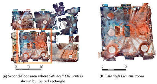
Figure 2.
RGB point cloud plan view of the southeast corner of Palazzo Vecchio (units in meters).
Sala degli Elementi has been previously investigated to assess damage through high-resolution imagery, ground-penetrating radar, infrared thermography, and GBL [29,30]. Wood et al. used Gigapan Epic Pro robotic panoramic platform to collect a total of 70 images of the walls of Sala degli Elementi and perform manual crack mapping after correcting the images for distortion, as shown in Figure 3 [29]. Wood et al. also collected lidar scans using a Faro Focus 3D X120 GBL platform, and a total of 15 GBL scans were collected from the second floor, seven of which were collected in Sala degli Elementi to minimize the occlusion. While most of the lidar scans were collected with a resolution setting of 1:4 and quality of 4×, one lidar scan conducted at the center of Sala degli Elementi with a higher resolution (resolution setting of 1:2 and quality of 4×), which resulted in a point cloud with an average point to point spacing of 1 mm [29]. Wood et al. employed the lidar-derived point cloud to perform floor level assessment by assigning the elevation of zero to the lowest point of the floor. The authors have reported that the result of floor level analysis matched the observed pattern of damage, which was due to structural retrofits applied to the structure. This finding was similarly observed in a follow-up study conducted by Napolitano et al. using a GBL and high-resolution thermal imaging using FLIR A615 camera to detect cracking within the walls of Sala degli Elementi [30]. However, it was reported that the width of cracks was approximated. Within the study, a total of six lidar scans and 72 thermal images were collected. To identify the cracks, the thermal images were registered to lidar data based on a method proposed by Hess et al. [31]. However, it was noted that only some of the cracks were visible in the thermal images.
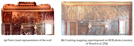
Figure 3.
East wall of Sala degli Elementi.
In this manuscript, the seven lidar scans collected by Wood et al. [29] from Sala degli Elementi are used for analysis. The lidar scans were registered using the Faro Scene software version 2020.0.5. The registration process was initially conducted based on visual matching, which enables an approximate alignment with high registration errors. Once the scans were roughly aligned, the registration process was further optimized via a cloud-to-cloud optimization technique to minimize the registration error. This process resulted in a point cloud with a mean registration error of 1.8 mm and a maximum error of 6.1 mm. The final point cloud consisted of 740 million points.
3.2. Overview of the Damage Detection Method
The point cloud damage detection method presented in this study is proposed by Mohammadi et al. [9]. Within the study, the authors proposed a damage detection workflow based on a pattern recognition approach and used only local geometric features to identify the damaged points with a point cloud irrespective of input point clouds underlying geometry. This section briefly discusses this method which consisted of three stages, preprocessing, extraction of damage-sensitive features, and classification (Figure 4).
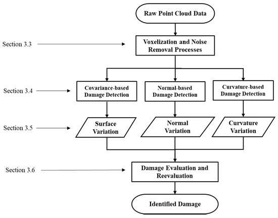
Figure 4.
Synopsis of the proposed methodology by Mohammadi et al. [9].
3.3. Preprocessing
Mohammadi et al. proposed workflow starts by regularizing the point-to-point spacing (i.e., point density or point cloud resolution) within the point cloud data through a voxelating process where a representative centroidal point is computed and used to represent all the points within a voxel [9]. Afterward, the sparse and erroneous points are eliminated through a statistical outlier removal [32]. The workflow’s damage-sensitive features are then computed based on exploiting each point’s local spatial distribution with respect to its neighboring points using two spatially invariant and one direction-wise feature. The idea here is that the points in the point cloud’s damaged areas have a different spatial distribution compared to the undamaged areas.
3.4. Extraction of Damage-Sensitive Features
The first computed feature is the covariance-based damage-sensitive feature. This feature is based on eigenvalues of each point and its selected neighboring points covariance matrix. Therefore, the workflow performs an eigendecomposition for each point and its selected neighboring points covariance matrix and then computes the corresponding eigenvalues. Afterward, the smallest eigenvalue ratio with respect to the summation of all eigenvalues is calculated and reported as the surface variation value [33]. The second damage-sensitive feature is computed based on each point’s normal vector variation with respect to a reference vector. The normal vectors are computed based on the weighted average method, where the weights are computed according to the area of adjacent triangles as described by Jin et al. [34]. As for the reference vector, the developed method can use two reference vectors based on the input point cloud’s geometry. The local reference vectors are created for each point and its selected closest neighboring points based on the eigenvectors resulting from the covariance matrix eigendecomposition. On the other hand, the global reference vector is identified based on eigenvectors resulting from the eigendecomposition of the covariance matrix of entire input point cloud. The third damage-sensitive feature is computed based on the mean curvature for each point to its selected closest neighboring points. The mean curvature within this study is computed based on averaging the curvature in vertical and horizontal directions of the global coordinate system. Mohammadi et al. compute the curvature in each direction by initially slicing the point cloud into segments parallel to vertical and horizontal directions based on the resolution selected for the voxelating process. Afterward, the algorithm identifies the osculating circle for each point and its selected closest neighboring points and estimates each segment’s curvature. As a result, for each point, the algorithm will estimate two curvature values (per each direction). Lastly, the average or one of these computed curvature values is considered as the third damage-sensitive feature.
3.5. Damage Evaluation and Reevaluation
Once the three features are computed, the classifier initially categorizes the points based on each feature as potential damaged and undamaged classes. This is conducted through estimating the Kernel Probability Distribution Function (PDF), where a point is considered as damage if its computed feature value probability is equal to or larger (or smaller depending on the skewness value of the PDF) than the probability of the PDF’s inflection point [35]. Once the points are classified into undamaged and potentially damaged categories based on each damage-sensitive feature, a damage identifier (DI) of 0 or 1 is assigned to each point, where 0 and 1 indicate undamaged and damaged classes, respectively. Then, the damage evaluation step evaluates each point’s DIs and classifies a point as a damaged point if and only if the point is considered as damage by all damage-sensitive features. Lastly, the workflow refines the damage detection results in the damage reevaluation step by reassessing the points one additional time to compare its classification with its eight neighboring points. As a result, each point classification is updated as damage if and only if 75% or more of its eight closest neighboring points were classified as damage. Then, the classifier categorizes the damaged points into a selected number of confidence intervals to illustrate the detection algorithm’s inherent uncertainty. The confidence intervals are determined based on each point’s damage probability, computed based on the median probability values that correspond to each damage-sensitive feature. Therefore, the points are categorized into selected bins that represent the median confidence intervals.
3.6. Detected Damage Segmentation
As stated, the proposed workflow to detect damage by Mohammad et al. [9] is able to detect and locate the damaged areas; however, it cannot separate the damaged regions into individual damaged parts for further analyses. As a result, a new and additional processing step is added to further categorize the damaged areas into individual segments within this study. The damage characterization method proposed within this study utilizes the analyzed point clouds containing potentially damaged areas. Afterward, the developed workflow uses a density-based clustering algorithm based on ordering points to identify clustering structures (OPTICS) to categorize the detected damaged regions [36]. OPTICS is an unsupervised learning classifier and does not require a predefined number of clusters similar to that of the k-means clustering algorithm [37]. The OPTICS classifier only requires two input parameters: the minimum number of points and the maximum distance needed to create a cluster. The advantage of the OPTICS classifier is that it can detect clusters with varying shapes and spatial distribution in 3D space, making it suitable to classify damaged areas that exhibit random patterns, and there is no prior knowledge existing of how many damaged areas are presented within the ROI.
3.7. Performance Evaluation of the Method
As the team could not perform a manual inspection from the walls in the Sala degli Elementi, the performance of the developed method was investigated based on another dataset that was collected from a historic religious structure located in Lincoln, Nebraska. The dataset was collected using a Faro Focus S350 GBL platform, and the laser scanner was placed at a distance of fewer than 4 meters from the cracking. The team minimized the offset angle between the GBL platform and the ROI. The scanner setting chosen to collect data was 1:4—4×, which resulted in a point cloud with a point-to-point spacing of less than 5 mm. Note that the parameter 4× within the scanner setting controls the number of measurements (oversampling) and does not contribute to the collected point cloud dataset point density. The selected segment is shown in Figure 5a. The chosen segment consisted of 11,600 points and was chosen as it demonstrates cracking damage similar to that observed within the Sala degli Elementi. The cracking had a varied width of approximately 1.5 cm at the top to 0.60 cm at the bottom. To analyze this dataset, initially, the data were voxelated with a grid step of 5.0 mm. It was then analyzed based on the eight closest points for surface variation, normal vector variation based on local reference planes (as the selected segment was curved surface), and curvature-based damage-sensitive features. As demonstrated in Figure 5c,d, the method could detect cracking of the selected segment. The precision for all confidence intervals was approximately 20 percent, while the recall value was 100 percent, where the precision for the cracked area was 70 percent.
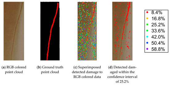
Figure 5.
Point cloud representation of the test specimen used for the evaluation study.
4. Discussion and Results
4.1. Analysis Results
To assess the workflow performance in detecting and segmenting the cracks, defects, and other surface anomalies, two segments of the Sala degli Elementi’s east wall are selected and analyzed in this manuscript (Figure 6 and Figure 7). The selected ROIs were extracted from the single high-resolution scan that was collected at the center of the room with the resolution setting of 1:2 and quality of 4× to eliminate inaccurate detections due to registration error. The ROIs are comprised of a predominantly planar surface, but this wall does contain local nonplanar deformities. Segment A is close to the southeast corner of the room, and segment B represents the entire top portion of the wall [28,29]. As illustrated in Figure 3b, Figure 6c, and Figure 7b, the selected ROIs sustained multiple cracking at centimeter and millimeter levels, identified through manual crack analysis of the images. In addition, it was noted that the walls represented many nonuniformities in out-out-plane protuberances at various locations.
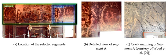
Figure 6.
Selected segments for analysis from the east wall of Sala degli Elementi.
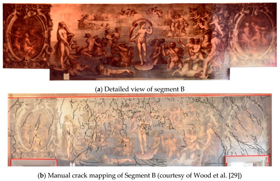
Figure 7.
Details of the selected second segment for analysis.
The point cloud representation of segment A contained approximately 1.5 million points and was analyzed for 5 mm or 10 mm surface anomalies. As a result, the cloud was voxelated using 5 mm and 10 mm dimension cubes during the preprocessing step. Segment B contained approximately 7 million points and was analyzed for 10 mm or larger cracking and other surface anomalies. Therefore, Segment B was only voxelated using 10 mm dimension cubes. The surface variation (or covariance-based), normal vector-based, and direction-wise (or curvature-based) damage-sensitive features were then utilized based on 8, 8, and 2 closest neighboring points, respectively. Note that as the selected regions contained localized bulges, as it is not entirely planar, the reference vectors were computed based on local planes that were identified based on 24 closest neighboring points. The neighboring number of 24 was found empirically and used to compute the local reference planes as this minimized the surface imperfections while enabling the workflow to detect cracking that resulted in a change in local geometry. Figure 8 depicts the estimated PDF for the surface variation and normal vector variations with respect to local reference planes that damage-sensitive features resulted during the point cloud analysis with 5 mm resolution. Once the features were computed, the damage evaluation and reevaluation steps identified the potentially damaged areas. The identified damaged points were then classified into 11 intervals. The analysis results for segment A based on three damage-sensitive features are shown in Figure 9a,b. After evaluating the damage detection results based on each damage-sensitive feature, it was observed that surface variation-based and curvature-based features are predominately able to detect surface imperfections and nonuniformities.
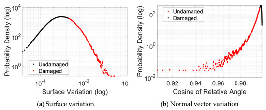
Figure 8.
Example log-log scaled PDF identifying undamaged and damaged points.
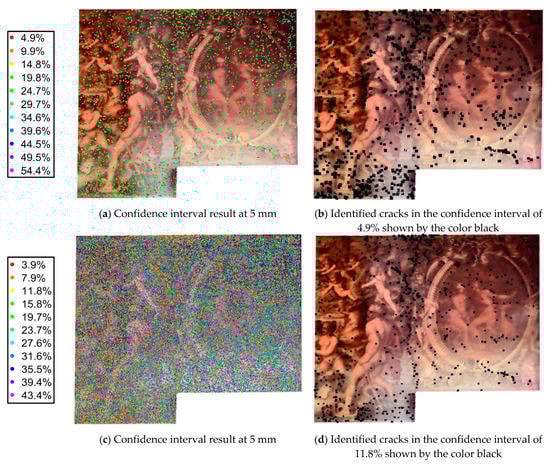
Figure 9.
Point cloud analysis results of segment A: detected damaged areas based on (a,b) three damage-sensitive features and (c,d) the normal-based damage-sensitive feature only.
In contrast, the detected damaged areas based on the normal-based features could locate the cracking with higher accuracy (Figure 9c,d). This was primarily concluded based on a qualitative analysis of the results of detected cracking areas at the selected confidence intervals with the manual crack mapping, as shown qualitatively in Figure 3, as no ground truth dataset exists for this dataset. However, the confidence interval analysis supports this conjecture. When using three damage-sensitive features to detect damaged areas, the first confidence interval contains the majority of features corresponding to cracking and several minor surface defects and nonuniformities present. Conversely, when only normal-based damage-sensitive features are considered, the first two confidence intervals need to be used to identify the cracks while fewer surface nonuniformities are present.
As a result, the crack detection process was investigated based on the normal-based damage-sensitive features. Figure 10 and Figure 11 represent the analysis result of segment A and segment B that are voxelated at 10 mm grid steps, respectively. The detected damaged areas are then classified into 16 confidence intervals allowing to isolate further the features that primarily represent the detected cracking areas. Figure 10a and Figure 11a depict the superimposed detected damaged areas for segments A and B based on all confidence intervals, respectively. Figure 10a,b and Figure 11b illustrate the superimposed detected cracking for segments A and B, respectively, based on the first three confidence intervals. As shown in Figure 10a,b and Figure 11b, while the damage detection method minimized the detection surface nonuniformities, some of the surface nonuniformities that represent feature values similar to that of cracking were classified as cracking. As a result, and to separate the cracking, the detected areas from segments A and B were further analyzed through the OPTICS clustering method as introduced in Section 3.6. To implement the OPTICS clustering process, two input parameters required the inclusion of the minimum number of points and the maximum distance. The minimum number of points to create a cluster and the maximum distance in this study were set to four points and 10 mm, respectively, and determined empirically. As shown in Figure 10c and Figure 11c, the clustering algorithm was able to segment the detected cracking.
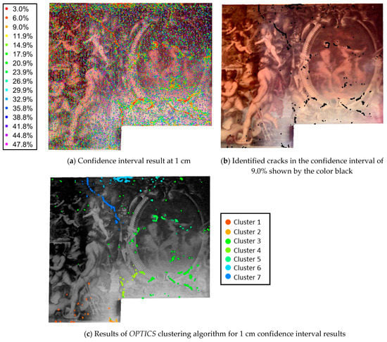
Figure 10.
Point cloud analysis results of the top right corner sustained cracking based on the normal-based damage-sensitive feature.
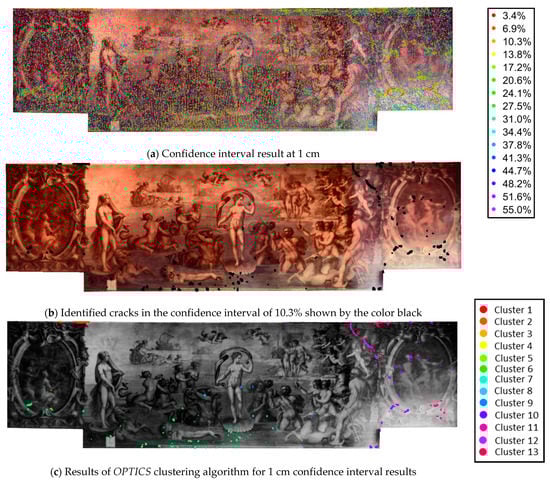
Figure 11.
Analysis results for segment B.
4.2. Performance Analysis
The method used within this study to detect the cracking areas utilizes local geometrical descriptors as damage-sensitive features. Therefore, only the cracks that create a change in geometry can be detected from point clouds. These changes in local geometry can be represented by the points laid in a distinctive pattern from that of the wall [12]. However, not all the observed and identified cracks identified manually are represented by such changes within the walls of Sala degli Elementi, which includes cracks with small widths. Therefore, only detected cracks within the point cloud data that result in local geometrical changes of 5 mm or higher can be qualitatively compared to that identified by Wood et al. [29]. Moreover, as Laefer et al. reported, crack widths of at least 5 mm or larger can be reliably detected from lidar-derived point clouds assuming the GBL platform location was optimal during the data collection. As a result, the selected segments were voxelated based on 5 mm and 10 mm grid steps, which resulted in the detectability of cracks with geometrical variations of 5 mm and 10 mm or larger, respectively. While Mohammadi et al. [9] provided a detailed discussion on how to select the input parameters for the damage detection method, a brief discussion is presented here for the normal vector feature that is used to detect the cracking areas. Within this study, the neighboring number of eight was used to compute the normal vectors. Within the voxelated point cloud, the eight neighboring points correspond to eight vertices located with the distance of one voxelating gird step (i.e., 5 mm or 10 mm). As a result, these features were assessing the spatial or geometric variation of each point with respect to the points that are located at 5 mm or 10 mm.
Following identifying the detected cracking areas, various damage confidence intervals are evaluated for the 5 mm and 10 mm segments. As each of these intervals essentially captures similar spatial distributions, the goal here is to identify the confidence interval that captures the spatial distribution of the points that correspond to the cracking. The goal of evaluating these intervals is to identify the confidence interval that represents the cracking while minimizing the presence of surface anomalies and bulges, which allows comparing the detected damaged regions with manual crack mapping results, as shown in Figure 6c and Figure 7b. Figure 9d, Figure 10b, and Figure 11b show superimposed detected damaged regions of the first three confidence intervals into the colored point cloud, representing the significant diagonal cracking identified from the images based on manual analysis. Moreover, it was noted that the selected confidence intervals for the spatial resolutions of 5 mm also represent major surface defects and localized bulges, potentially due to humidity or construction style, within the bottom of the selected ROI. However, by comparing Figure 9c,d, Figure 10a,b, and Figure 11a,b, it can be observed that the majority of the minor surface defects and anomalies, shown by the other confidence intervals, can be distinguished and eliminated as large cracks. Based on the detailed comparison for segment A analysis results at 5 mm, it was observed that the developed method was able to identify two of the diagonal shear cracking at the top of the segment (shown by A and B in Figure 12) as well as vertical cracking at the top left of the doorway (shown by C in Figure 12) and shear cracking at the right of the entrance (shown by D in Figure 12). Additionally, it was noted that some of the smaller cracks at the middle of the segment were identified.
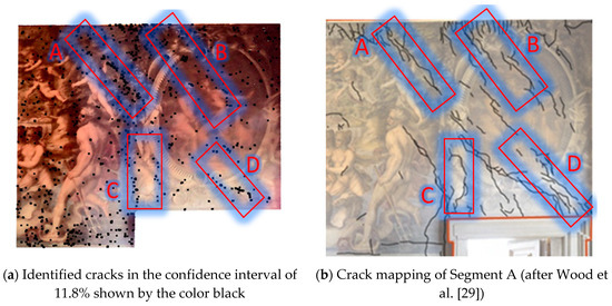
Figure 12.
Comparison of detected damaged areas with the manual crack mapping.
4.3. Discussion
The developed method within this study uses local geometric variations computed based on voxelated point cloud to identify the damaged areas. Consequently, the detection is limited to the cracks and other surface defects that result in a change in geometry equal to or larger than that of voxelating grid step size. For example, the analysis results of segments A and B at 10 mm demonstrates that the developed method was able to identify cracks that result in local geometry change of 10 mm or larger. This includes the significant shear cracking at the top right of the wall (shown by A in Figure 12), highlighted by cluster 7 in Figure 10c and cluster 12 in Figure 11c. Furthermore, only a section of the vertical cracking (shown by C in Figure 12), the shear cracking on the top right of the doorway (crack D in Figure 12), and a portion of the cracking at the left and middle walls (clusters 1, 5, and 6 in Figure 11c) were detected. While other studies, such as Valenca et al. or Hou et al. [7,16], demonstrate workflows that can detect cracking with a higher level of accuracy, these methods rely on crack detection based on intensity or color information, which is not ideal for fresco walls, particularly within Sala degli Elementi.
5. Conclusions
This manuscript analyzed the lidar-derived point clouds of a culturally prominent structure, Palazzo Vecchio, through evaluating and expanding the damage detection and characterization workflow proposed by Mohammadi et al. [9]. The lidar data were collected from one room, known as Sala degli Elementi. The damage detection method evaluated within this study uses three damage-sensitive features to detect surface damage and cracks from the point clouds at the three separate resolutions. The method combines these three surface feature descriptors that are invariant to the point cloud’s underlying geometry, which results in a more scalable damage detection algorithm that does not rely on color or intensity data from a lidar scanner or supplemental sources. Furthermore, the developed method classifies the detected damaged areas into a selected number of confidence intervals. Through detailed evaluation of results based on each damage-sensitive feature, it was observed that only the normal-based damage-sensitive features were able to detect the cracking and minimize the presence of surface anomalies and bulges. Therefore, only normal-based damage-sensitive results were used within this study. Furthermore, to separate the detected cracking from the surface anomalies that represent feature values similar to that of cracking areas, a workflow based on the OPTICS clustering method was used.
To validate the workflow’s performance and scalability, two-point cloud segments of the east wall of Sala degli Elementi that sustained heavy cracking were evaluated at two resolutions and qualitatively compared with crack mapping conducted based images through manual analysis. This was done as the team could not perform crack assessment and quantify data due to access limitations. The selected segment represents a predominately planar surface. As reported by Laefer et al. and observed based on the analysis results of the wall segments within this study, it can be concluded that GBL-derived point clouds can be used to detect cracking of size 5 mm or higher that results in a change in local geometry [11,12]. However, various nonuniformities existed throughout its surface. The damage detection analysis was performed at two different spatial resolutions of 5 mm and 10 mm. The detected damaged areas are further classified into multiple confidence intervals. The detected damaged areas demonstrated that the developed method could detect not only the cracking but also all minor surface anomalies, making visualizing and detecting cracking difficult at this initial stage. As a result, the various confidence intervals were investigated. It was determined that the first three intervals for both spatial resolutions could depict the cracking while minimizing the presence of detected surface anomalies. Moreover, the identified damaged areas included cracking and other surface nonuniformities, were further separated using the OPTICS clustering algorithm for both segments at a 10 mm resolution, which enabled direct comparison of the detected crack with manual crack mapping results.
The analysis results demonstrated if the cracking results in local geometric changes equal to or greater to that of the voxelization grid step, the proposed method can be used to detect these defected areas. However, it was noted that minor surface anomalies that represent feature values similar to that of cracking could be classified with cracking, in particular for resolution or voxelating gird steps of 5 mm. A segmentation step was proposed to combat the issue and isolate the larger cracks of interest. This workflow enables a more objective comparison between the manual cracking mapping and identified areas using the workflow. However, a number of limitations were identified within this study. The first limitation of this study corresponds to the type of features used within this study. As the damage-sensitive features used within this study are developed based on identifying changes in local geometric features, these are susceptible to point density and its variation within a point cloud. While the point density variation effect is minimized through the voxelating process (as suggested by Mohammadi et al. [9]), the smaller voxelating grid steps may not reduce the point density variation in comparison to a larger grid step. This can be observed based on comparing the damage detection results of segment A at 5 mm to 10 mm resolutions. The second limitation of this study corresponds to isolating the cracks from surface nonuniformities. While the OPTICS clustering algorithm separated the primary shear cracking from other defects, most sparse detections were grouped with cracked areas. As a result, the primary future research direction includes developing a method to improve the clusters via region growing. This can be done by considering the location and other surface similarities and enabling direct quantifying the damaged area, including area, depth, length, and width based on the segmented damaged regions.
Author Contributions
Data curation, R.L.W.; Formal analysis, R.L.W. and M.E.M.; Methodology, R.L.W. and M.E.M.; Project administration, R.L.W.; Supervision, R.L.W.; Validation, R.L.W. and M.E.M.; Writing—original draft, R.L.W. and M.E.M.; Writing—review and editing, R.L.W. and M.E.M. All authors have read and agreed to the published version of the manuscript.
Funding
No external funding directly supports this work.
Institutional Review Board Statement
Not applicable.
Informed Consent Statement
Not applicable.
Acknowledgments
Lidar data used within the study were collected under the support of the National Science Foundation under IGERT Award #DGE-0966375 “Training, Research and Education in Engineering for Cultural Heritage Diagnostics”. Additionally, the authors would like to thank Christine Wittich, Falko Kuester, Maurizio Seracini, Francesco Tioli, Patrizio Mannucci, and Stefano Corazzini, for their support during the original field survey.
Conflicts of Interest
The authors declare no conflict of interest. In addition, the funders had no role in the design of the study, in the collection, analyses, or interpretation of data, in the writing of the manuscript, or in the decision to publish the results.
References
- Park, H.S.; Lee, H.M.; Adeli, H.; Lee, I. A new approach for health monitoring of structures: Terrestrial laser scanning. Comput.-Aided Civ. Infrastruct. Eng. 2007, 22, 19–30. [Google Scholar] [CrossRef]
- Olsen, M.J.; Kuester, F.; Chang, B.J.; Hutchinson, T.C. Terrestrial laser scanning-based structural damage assessment. J. Comput. Civ. Eng. 2009, 24, 264–272. [Google Scholar] [CrossRef]
- Erkal, B.G.; Hajjar, J.F. Laser-based surface damage detection and quantification using predicted surface properties. Autom. Constr. 2017, 83, 285–302. [Google Scholar] [CrossRef]
- Axel, C.; van Aardt, J.A. Building damage assessment using airborne lidar. J. Appl. Remote Sens. 2017, 11, 046024. [Google Scholar] [CrossRef]
- Mohammadi, M.E. Point Cloud Analysis for Surface Defects in Civil Structures. Ph.D. Thesis, University of Nebraska-Lincoln, Department of Civil Engineering, Lincoln, Nebraska, 2019. [Google Scholar]
- Kashani, A.G.; Olsen, M.J.; Graettinger, A.J. Laser scanning intensity analysis for automated building wind damage detection. Comput. Civ. Eng. 2015, 2015, 199–205. [Google Scholar]
- Hou, T.C.; Liu, J.W.; Liu, Y.W. Algorithmic clustering of LiDAR point cloud data for textural damage identifications of structural elements. Measurement 2017, 108, 77–90. [Google Scholar] [CrossRef]
- Olsen, M.J. In situ change analysis and monitoring through terrestrial laser scanning. J. Comput. Civ. Eng. 2015, 29, 04014040. [Google Scholar] [CrossRef]
- Mohammadi, M.E.; Wood, R.L.; Wittich, C.E. Non-temporal point cloud analysis for surface damage in civil structures. ISPRS Int. J. Geo-Inf. 2019, 8, 527. [Google Scholar] [CrossRef]
- Nace, T. We Have Beautiful 3-D Laser Maps of Every Detail of Notre Dame. Available online: https://www.forbes.com/sites/trevornace/2019/04/16/we-have-beautiful-3d-laser-maps-of-every-detail-of-notre-dame/?sh=4e3e887226e6 (accessed on 22 March 2021).
- Laefer, D.F.; Gannon, J.; Deely, E. Reliability of crack detection methods for baseline condition assessments. J. Infrastruct. Syst. 2010, 16, 129–137. [Google Scholar] [CrossRef]
- Laefer, D.F.; Truong-Hong, L.; Carr, H.; Singh, M. Crack detection limits in unit based masonry with terrestrial laser scanning. Ndt E Int. 2014, 62, 66–76. [Google Scholar] [CrossRef]
- Chen, S.; Laefer, D.F.; Byrne, J.; Natanzi, A.S. The effect of angles and distance on image-based, three-dimensional reconstructions. In Safety and Reliability: Theory and Applications; CRC Press: Boca Raton, FL, USA, 2017; pp. 2757–2761. [Google Scholar]
- Torok, M.M.; Golparvar-Fard, M.; Kochersberger, K.B. Image-based automated 3D crack detection for post-disaster building assessment. J. Comput. Civ. Eng. 2013, 28, A4014004. [Google Scholar] [CrossRef]
- Kim, M.-K.; Sohn, H.; Chang, C.-C. Localization and quantification of concrete spalling defects using terrestrial laser scanning. J. Comput. Civ. Eng. 2014, 29, 04014086. [Google Scholar] [CrossRef]
- Valença, J.; Puente, I.; Júlio, E.; González-Jorge, H.; Arias-Sánchez, P. Assessment of cracks on concrete bridges using image processing supported by laser scanning survey. Constr. Build. Mater. 2017, 146, 668–678. [Google Scholar] [CrossRef]
- Vetrivel, A.; Gerke, M.; Kerle, N.; Nex, F.; Vosselman, G. Disaster damage detection through synergistic use of deep learning and 3D point cloud features derived from very high resolution oblique aerial images, and multiple-kernel-learning. ISPRS J. Photogramm. Remote Sens. 2018, 140, 45–59. [Google Scholar] [CrossRef]
- Womble, J.A.; Wood, R.L.; Mohammadi, M.E. Multi-scale remote sensing of tornado effects. Front. Built Environ. 2018, 4, 66. [Google Scholar] [CrossRef]
- Qi, C.R.; Su, H.; Mo, K.; Guibas, L.J. Pointnet: Deep learning on point sets for 3d classification and segmentation. In Proceedings of the IEEE Conference on Computer Vision and Pattern Recognition, Honolulu, HI, USA, 21–26 July 2017; pp. 652–660. [Google Scholar]
- Nasrollahi, M.; Bolourian, N.; Hammad, A. Concrete surface defect detection using deep neural network based on lidar scanning. In Proceedings of the CSCE Annual Conference, Laval, QC, Canada, 12–15 June 2019. [Google Scholar]
- Wang, Y.; Sun, Y.; Liu, Z.; Sarma, S.E.; Bronstein, M.M.; Solomon, J.M. Dynamic graph cnn for learning on point clouds. ACM Trans. Graph. 2019, 38, 1–12. [Google Scholar] [CrossRef]
- Haurum, J.B.; Allahham, M.M.J.; Lynge, M.S.; Henriksen, K.S.; Nikolov, I.A.; Moeslund, T.B. Sewer Defect Classification using Synthetic Point Clouds. In Proceedings of the 16th International Conference on Computer Vision Theory and Applications (VISAPP), Vienna, Austria, 8–10 February 2021. [Google Scholar]
- Barnett, V.; Lewis, T. Outliers in statistical data. In Wiley Series in Probability and Mathematical Statistics. Applied Probability and Statistics; Wiley: Hoboken, NJ, USA, 1984. [Google Scholar]
- Kashani, A.G.; Graettinger, A.J. Cluster-Based Roof Covering Damage Detection in Ground-Based Lidar Data. Autom. Constr. 2015, 58, 19–27. [Google Scholar] [CrossRef]
- Girardeau-Montaut, D.; Roux, M.; Marc, R.; Thibault, G. Change detection on points cloud data acquired with a ground laser scanner. Int. Arch. Photogramm. Remote Sens. Spat. Inf. Sci. 2005, 36, W19. [Google Scholar]
- Lague, D.; Brodu, N.; Leroux, J. Accurate 3D comparison of complex topography with terrestrial laser scanner: Application to the Rangitikei canyon (NZ). ISPRS J. Photogramm. Remote Sens. 2013, 82, 10–26. [Google Scholar] [CrossRef]
- Ottoni, F.; Blasi, C. Results of a 60-year monitoring system for Santa Maria del Fiore Dome in Florence. Int. J. Archit. Herit. 2015, 9, 7–24. [Google Scholar] [CrossRef]
- Alessandri, C.; Cappelli, E.; Leggeri, B.; Muccini, U.; Tralli, A. Critical discussion about some measurements on a damaged corner of Palazzo Vecchio. In Structural Studies of Historical Buildings IV. Volume 1: Architectural Studies, Materials and Analysis; Canadian Conservation Institute: Ottawa, ON, Canada, 1995; pp. 37–44. [Google Scholar]
- Wood, R.L.; Hutchinson, T.C.; Wittich, C.E.; Kuester, F. Characterizing Cracks in the Frescoes of Sala degli Elementi within Florence’s Palazzo Vecchio. In Euro-Mediterranean Conference; Springer: Berlin/Heidelberg, Germany, 2012; pp. 776–783. [Google Scholar]
- Napolitano, R.; Hess, M.; Glisic, B. Integrating non-destructive testing, laser scanning, and numerical modeling for damage assessment: The room of the elements. Heritage 2019, 2, 12. [Google Scholar] [CrossRef]
- Hess, M.; Vanoni, D.; Petrovic, V.; Kuester, F. High-resolution thermal imaging methodology for non-destructive evaluation of historic structures. Infrared Phys. Technol. 2015, 73, 219–225. [Google Scholar] [CrossRef]
- Rusu, R.B.; Marton, Z.C.; Blodow, N.; Dolha, M.; Beetz, M. Towards 3D Point cloud based object maps for household environments. Robot. Auton. Syst. 2008, 56, 927–941. [Google Scholar] [CrossRef]
- Pauly, M.; Gross, M.; Kobbelt, L.P. Efficient simplification of point-sampled surfaces. In Proceedings of the IEEE Visualization, Boston, MA, USA, 27 October–1 November 2002; pp. 163–170. [Google Scholar]
- Jin, S.S.; Lewis, R.R.; West, D. A comparison of algorithms for vertex normal computation. Vis. Comput 2005, 21, 71–82. [Google Scholar] [CrossRef]
- Shalizi, C. Advanced Data Analysis from an Elementary Point of View; Cambridge University Press: Cambridge, UK, 2013. [Google Scholar]
- Ankerst, M.; Breunig, M.M.; Kriegel, H.-P.; Sander, J. OPTICS: Ordering points to identify the clustering structure. ACM Sigmod Rec. 1999, 28, 49–60. [Google Scholar] [CrossRef]
- Hartigan, J.A.; Wong, M.A. AK—means clustering algorithm. J. R. Stat. Soc. 1979, 28, 100–108. [Google Scholar]


Publisher’s Note: MDPI stays neutral with regard to jurisdictional claims in published maps and institutional affiliations. |
© 2021 by the authors. Licensee MDPI, Basel, Switzerland. This article is an open access article distributed under the terms and conditions of the Creative Commons Attribution (CC BY) license (https://creativecommons.org/licenses/by/4.0/).