1. Introduction
Chasing (ciselure in French) is a metalworking technique in which a tool is hammered on the front side of a metal by using tools called liners and punches—of many shapes and sizes—and a small hammer. Chasing is one of the most widely used methods of metalworking due to its relative simplicity and flexibility; it can be used on a wide range of objects, from small jewellery pieces to large sculptural works [
1]. Chasing is a technique that has not changed vastly across periods or geographical regions, and it is found in a wide variety of objects with origins ranging from the Tang dynasty in China (
Figure 1) to ornaments from the Boulle furniture at the Louvre [
2]. Each chaser fabricates their own tools; thus, identifying the tool used on an object based on the chasing imprint is of great interest for archaeologists, art historians, and conservators, as it can provide valuable information on the provenance of the object, its fabrication method, and its
chaîne opératoire. The profile of the imprint left by a liner is distinctive from those of other metalworking techniques, such as engraving, as it has a
U-shaped profile. Since the tool is hammered on the surface of the metal, there is no loss or waste of material, as the excess material is displaced to the borders of the surface, leaving a visible toolmark.
Quantitative analysis has been performed on toolmarks found in different objects, such as sculptures [
3], rock-art [
4], and engraved bones [
5], but not on chased metal objects. This analysis is mostly based on the surface topologies obtained by different means of acquisition, such as 3D scanners, digital microscopy, or microtopography. Optical microtopography is a non-invasive, non-contact technique in which the surface of an object is scanned with microscopic precision to allow its metrical characterisation.
This paper aims to quantitatively use microtopographic data to analyse the morphologies of imprints left by different chasing tools. In order to examine the different toolmarks, experimental chasing marks were made on brass and copper metal plates. These metal plates were scanned using microtopography, and the morphologies of the imprints were quantified to classify and identify the tool that produced each imprint.
Archaeological metal objects are normally found in weathered conditions, so to evaluate the feasibility of this method on real objects, the mock-ups were artificially aged, and the same methodology was applied to them. This methodology could potentially be used to study real objects and identify which tools were used for their fabrication.
The structure of this paper is as follows: The next section will present a brief background on chasing as a metalworking technique and a brief literature review on toolmark analysis, and the third section will describe the fabrication of the mock-ups, the artificial ageing method, the microtopography acquisition device, and the morphological analysis of the toolmarks. The fourth section will present and discuss the results obtained for the reference and aged mock-ups. Finally, concluding remarks will be presented in the fifth section.
3. Materials and Methods
3.1. Fabrication of Chasing Mock-Ups
For the purpose of this research, chasing mock-ups were made by a professional chaser. Two different types of metal were used—brass and copper, which are representative of many chased metal objects. Different metals have a different malleability; hence, it is of interest to compare differences and similarities in chasing imprints on different metals.
There are two main categories of chasing tools, matting punches and liners (
Figure 2). The former are used to embellish a surface by modifying its surface roughness. Different appearances, called colours, can be achieved by changing the roughness of the surface. Frequently, these tools give the surface a matte appearance; hence, their name. The latter are used to draw lines around the object. Different liners are used to obtain different line thicknesses; narrow liners are used on smaller designs. A range of arched liners are used for curved lines, depending on the desired curvature of the design. Thus, for a single drawing, a wide variety of tools are used, and if elaborated by a professional, the transition between one tool to the other should be imperceptible to the naked eye. For this paper, only liners will be studied, as they produce a clear profile. Matting punches give very different surface appearances that are easily distinguishable by the naked eye. For this paper, seven liners were used: three straight liners with varying thicknesses and four curved liners with different curvatures (
Figure 3). The tool names and descriptions are presented in
Table 1.
The mock-ups were made according to the following steps:
The desired design was drawn on the metal using a marker.
The metal was fixed to a pitch bowl by melting the pitch on the surface of the bowl using a blow torch and placing the metal in the desired position.
Once the pitch was cold and the metal was fixed, the pattern was chased using the desired liners or punches by pushing them against the metal with a chaser hammer.
When all of the patterns were chased, the metal was removed from the pitch bowl by heating the pitch. Any pitch remaining on the surface of the metal was burned with a blowtorch.
Artificial Ageing
The mock-ups were artificially aged by preparing an intentional patina. This was done by chemo-thermal means with an acetic acid at 10% (
v/
v) in an aqueous solution at 200°/300° Celsius in oxidising conditions by using a butane torch with pulsed air.
Figure 4 shows the mock-ups before and after ageing.
3.2. Microtopographic Data Acquisition
The microtopography of the mock-ups’ surfaces was acquired using an Altimet AltiSurf© 50, which uses optical sensors based on chromatic confocal sensing (CCS) (
Figure 5). This is a non-contact scanning technique that has a precision in the
plane of up to 500 nm. The acquired surface was analysed according to the ISO 25178 international standard for quantification and measurement [
4]. Microtopography measurements have a very high resolution, and the measurement precision in height is up to 5 nm. However, this method is very time consuming, as a 1 cm
2 measurement can take from 30 min at an 80
m spatial resolution to as long as 17 h at 500 nm [
5].
Microtopography is advantageous compared to other methods of acquisition, such as digital microscopy, which can present errors in transformation from texture to 3D. Moreover, the sequence of movements on engraving processes, line crossings, and modifications on the surface because of weathering, scraping, or rubbing are made visible and the precise morphology of the lines can be extracted [
5].
CCS works under the principle of chromatic sensing, in which a white beam of light is diffracted by a chromatic lens. The spectrum is incident on a point on the surface and reflected into a spectrophotometer. The peak in the reflected spectrum is encoded into the relative surface height.
The measurements were made with an 8 mm scanning sensor and a measuring step of 5 m in both the x and y directions. For each toolmark, four different areas were chosen to represent the whole trace and its evolution. The dimensions of the areas scanned ranged in size from 3 × 3 to 5 × 7 mm.
3.3. Processing Pipeline
3.3.1. Pre-Processing
The surface microtopography was pre-processed according to ISO 25178 standards. First, the surface had to be flattened by taking the average plane of the surface and setting its gradient to 0. Then, any non-measured points that could happen during the acquisition stage were filled by taking the average of the points in the vicinity (
Figure 6a). Since the samples were uniform, the number of non-measured points was minimal.
3.3.2. Extraction of Morphological Features
The surface microtopography was visualised and the desired profiles were selected by drawing a 300-point line that was equivalent to 1.5 mm (
Figure 6c). For each toolmark, 40 profiles are selected at different sections of the line. This was done to ensure that variations within one toolmark were considered and that the profiles selected for each tool were representative of the whole toolmark. Once the profiles were selected, they were filtered using an open Gaussian filter with a cut-off wavelength of 0.08 mm. This step was used to separate the roughness from the waviness profile according to the ISO 16610-21 standard (
Figure 6d).
The morphological features were taken according to the work of Bello et al. [
15]. In order to calculate the morphological features, seven landmark points were detected (labelled in
Figure 6e). These were the minimum (LM7), the maxima on both sides of the incision (LM1, LM2), the bottom points, which were defined as the profile points at 10% above the minimum (LM5, LM6), and the middle points at 50% above the minimum (LM3, LM4). From the landmark points, the morphological features could be calculated; these were the width at the incision surface (WS), the width at the bottom of the incision, which was 10% above the minimum (WB), and the width at 50% above the minimum (WM). The perpendicular depth (D) from the surface to the minimum was also calculated, as were the depths from the right (RD) and left (LD) maxima. The final morphological point was the opening angle of impact (OA) (
Figure 6f).
3.4. Statistical Analysis
The morphological features taken from the toolmark profiles can be analysed by using simple statistical tools for visualisation and characterisation. A Tukey boxplot is a visualisation method that describes the distribution of data through quartiles, dividing the data into four equal groups by using the median, upper, and lower quartiles, without assuming the statistical distribution of the data.
In order to evaluate if the distributions visualised in a Tukey boxplot belong to the same population or if they present statistically significant differences, a Wilcoxon rank-sum test can be performed. In the Wilcoxon rank-sum test, the null hypothesis H0 assumes that the distributions are equal. A p-value lower than 0.05 dismisses the null hypothesis with a 5% confidence, meaning that the groups are statistically different.
Finally, once the features have been analysed independently, they can be used to train a classification algorithm. The morphological features were used as a feature vector, where, for each toolmark, there were 40 samples and seven features. The Classification Learner Toolbox from Matlab [
19] was used to perform the classification with a 5-fold hold-out for validation. The Mahalanobis distance was favoured as a distance metric since it is unitless, scale-invariant, and takes into account the correlations in the dataset.
4. Results
4.1. Microtopographical Surface and Profile Analysis
The mock-ups were scanned using the microtopography setup, as described in
Section 3. Then, the mock-ups were artificially aged and re-scanned using the same procedure. Some examples of surface scans of different tools are presented in this subsection.
The first example is of tools I and J on brass before artificial ageing (
Figure 7). It is possible to observe that the surface roughness of the brass was smooth, and there was a homogeneous texture from the manufacturing process of the metal plate. A profile was extracted from each tool (
Figure 7c). A distinctive profile shape was present for both tools, yet there were clear differences. Tool I had a smaller surface width, and it had a
V-shape. J, on the other hand, had a wider surface width, and the incision was
U-shaped.
The same area was scanned after the artificial ageing (
Figure 8). There were clear differences in the surfaces before and after ageing. The surface roughness of the metal was much more irregular due to the artificial patina. The corrosion on the metal created areas of rust where oxides or salts appeared on the surface, causing the drawing on the surface to be less sharp. The profiles also showed a clear change after ageing (
Figure 8c).
There was a striking difference in profile shape after the artificial ageing. Both profiles became similar in shape after ageing. The shapes of the profiles before ageing were much sharper, whereas after ageing, they were more irregular, and both tools had a V-shape.
A similar effect was visible on all tools for both brass and copper before and after ageing (
Figure 9). In the case of both brass and copper, before ageing, each tool had a distinct shape. In the case of some tools, there was a large amount of excess metal displaced on the sides, which was the case of L, M, and N for brass and J, L, N, and O for copper.
For the aged mock-ups, the distinction between each tool decreased drastically. The profiles become more uniform in shape for both metals. Moreover, the sharp edges between the surface of the metal and the toolmark that were visible before ageing became smooth after ageing. In addition, the excess metal on the sides of the toolmark was completely corroded after ageing.
4.2. Statistical Analysis of Morphological Features
Both metals were scanned before and after ageing, and 40 profiles were taken for each tool. The landmark points defined by Bello et al. [
15] and defined in
Section 3 were detected for each profile, and the morphological descriptors were calculated accordingly (
Figure 10).
The boxplot shows the mean, quartiles, and outliers of each morphological feature for each tool in the four cases (brass and copper before and after ageing). In the case of brass before ageing, all features were quite representative of each tool and there were few outliers, except for tool M, which had some outliers for WS, WM, and WB. At some sections of the toolmark, its profile was shaped as if two consecutive taps were done with different forces, creating a deep and narrow incision and a shallow and wide one on the same spot. This could explain why the morphological features representative of width were not very uniform.
In the case of copper, outliers were present for I at WS, WM, and WB, as well as LD and RD. I was a tool used for small curvatures; thus, the sections belonging to the start and end of the incision were proportionally higher compared to those with other tools. Normally, at the start and end of the incision, the pressure applied was inconstant; therefore, the width could vary with respect to the rest of the toolmark.
Another feature that presented outliers in the case of copper was WB for tool O. WB represents the width at the bottom of the incision. Therefore, it could be assumed that O produced a less uniform incision, ranging from a U-shaped profile with a wide bottom to a more V-shaped profile with a narrower bottom.
LD and RD represent the lengths of the right and left sides of the incision. Since the mock-ups were not always scanned in the same position, left and right became relative descriptors, which could explain the presence of outliers for these features. This was mostly seen in the case of copper before ageing and the case of brass and copper after ageing.
Aged brass and copper showed outliers in WS and D (mostly in the case of aged copper) for many tools. This could be explained by the corrosion caused by the artificial ageing. Since the artificial patina generated a change in the surface roughness, WS would be greatly affected, as sections of the toolmark would have different levels of non-uniform rust, creating differences in the surface width. The depth would also be affected by the artificial ageing, as the bottom of the incision could also be affected by the non-uniform formation of rust.
Wilcoxon Rank-Sum Test
In order to evaluate if the overlaps in the Tukey boxplot were statistically significant, a Wilcoxon rank-sum test was performed for all the morphological features. Each feature obtained for each tool used in a specific mock-up was compared to each other one. The null hypothesis (H0) assumed that the pair of populations was the same, and a p-value lower than 0.05 indicated a rejection of H0, meaning there that there was a statistically significant difference between the two groups.
The
p-values calculated for all morphological features of all of the tools in non-aged brass and copper are presented in
Table 2 and
Table 3. For each morphological feature, there were a few tools that did not present statistically significant differences given a 5% confidence interval. These results coincided with those of the Tukey boxplots. For example, LD and RD presented many pairs of tools that were not statistically significantly different. As previously mentioned, these two features were the least robust, as they depended on the orientation in which the mock-ups were scanned.
In the case of brass (
Table 2), the most robust feature was WB, which only presented one pair (I vs. L) that did not reject H0. D and OA presented two pairs that did not reject H0: N vs. K and O vs. K in the case of D and I vs. J and N vs. K in the case of OA. WM, LD, and RD had the highest number of features that did not reject H0, making them the least characteristic features.
In the case of copper (
Table 3), the features were less statistically significant than they were for brass. RD was the most descriptive, with only one pair (I vs. L) not rejecting H0. LD had two pairs that did not reject H0 (O vs. J and N vs. K), suggesting that these mock-ups were always scanned in the same orientation. The least representative features were WS, WM, and WB, suggesting that the width of the profile, regardless of its location, was not very representative of the toolmark.
The
p-values calculated for the artificially aged mock-ups are presented in
Table 4 for brass and in
Table 5 for copper. In the case of aged brass, there were more pairs of tools that were statistically significantly different. I and J had the most similar features to those of other tools. D was the most representative morphological feature, as it only presented four pairs that did not reject H0.
In the case of aged copper, the features were also less characteristic of the toolmarks. The morphological features that presented the most statistically significantly similar pairs were RD and OA. As with aged brass, the most characteristic feature was D, which only had one pair of tools that do not reject H0.
In the case of both metals, before and after ageing, all morphological features and tools gave p-values that rejected H0. Even if there were specific pairs of tools that did not present statistically significant differences for specific morphological features, the same pairs did show statistically significant differences in other morphological features. Since the classification task was a multivariate analysis, all of the features were used.
4.3. Classification of Tools
The morphological features presented above were used to train a classification algorithm by using the Classification Learner Toolbox in Matlab [
19]. The models were trained with a five-fold cross-validation. The Matlab toolbox had the capability of training different models, and the model that gave the best results was a weighted K-nearest neighbours (KNN) model [
20] while using the Mahalanobis distance metric, 10 neighbours, and an inverse squared weight function. Other more complex models could have been trained, but given that the training set was small, this could have led to overfitting of the data.
4.3.1. Brass
The overall accuracy obtained for brass was 91%. The confusion matrix was calculated for all of the tools on brass before ageing (
Figure 11). All the tools were correctly identified with an accuracy higher than 90%, except for J and K, with 82.5% accuracy. All of the misclassified profiles belonging to J (17.5%) were incorrectly identified as I. Similarly, all of the misclassified profiles belonging to I (10%) were incorrectly classified as J. The morphological features obtained for both tools had a large overlap, which indicated that they produced similar profiles (
Figure 10). Moreover, the Wilcoxon rank-sum test showed that for I and J, 4/7 morphological features belonged to the same distribution (
Table 2). In the case of K, 12.5% of the profiles were incorrectly labelled as L, and the another 5% were empty misclassified as N and O. However, K and L only had one feature that was similar.
4.3.2. Copper
In the case of copper, the overall accuracy was 84%. The confusion matrix was calculated for all of the tools, except for M (
Figure 12). This was because during the acquisition, the data for M were not reliable, but, at the time when the data were analysed, the mock-ups had already been aged. Tools L, N, and O had an accuracy higher than 90%. The lowest accuracy was 67.5% for tool K, which was also the tool with the highest number of false positives (25%).
For I, most profiles (12.5%) were misclassified as J; conversely, for J, most profiles (12.5%) were misclassified as I. However, for these tools, all morphological features presented statistically significant differences. For J, 10% of the profiles were mislabelled as K. In the case of K, most profiles (12.5%) were misclassified as J, and the rest were mislabelled as L, N, and, to a lesser extent (5%), O. J and K also had many morphological features that overlapped, causing the algorithm to misclassify these two tools (
Figure 10). Moreover, the Wilcoxon rank-sum test showed that 3/7 features of J and K were statistically similar (
Table 3).
4.3.3. Aged Brass
For artificially aged brass, the overall accuracy was 65%. The accuracy decreased drastically after ageing. The confusion matrix was calculated for all tools (
Figure 13). The worst classification accuracies were for I (47.5%), L (50%), J (60%), and K (65%). The best classification was obtained for O (80%), N (77.5%), and M (75%).
The most significant misclassification was in the case of I, where 37.5% of the profiles were misidentified as N; however, only 7.5% of the N profiles were misclassified as belonging to I. N, together with J, was the tool with the highest false positive rate (45%). The Wilcoxon rank-sum test showed that, statistically, for these tools, their values of LD and OA were not significantly different (
Table 4). However, the Tukey boxplot showed that I had many outliers, especially for WS, LD, and RD, which could explain why its accuracy was so low (
Figure 10).
L also had a low accuracy of only 50%; however, it also had a low false positive rate of 20%. Furthermore, it was the class with fewest predictions overall—less than 10% of the toolmarks were predicted to belong to L. The Wilcoxon rank-sum test showed that for all possible pairs of tools and features (42), M had the most non-distinct features (18). Moreover, the Tukey boxplot showed that although L did not have many outliers, it is the tool with the widest spread for most features—notably, WM, D, and OA. This indicated that the morphological features were not well descriptive of tool L on aged brass.
4.3.4. Aged Copper
In the case of artificially aged copper, the overall accuracy was 68%. The confusion matrix was calculated for all of the tools (
Figure 14). The best accuracies were obtained for O (87.5%), J (85%), L (75%), and M (67.5%). The worst accuracies were obtained for I (47.5%), N (55%), and K (62.5%). The highest misclassification was in the case of N, where 30% of profiles were mislabelled as K. In addition, 27.5% of the K profiles were misclassified as belonging to N. The large confusion between K and N came from the fact that many of their morphological features overlapped (
Figure 10). Moreover, the Wilcoxon rank-sum test showed that K and N shared 4/7 features that were statistically significantly similar (
Table 5). Furthermore, K and N were the two tools with the highest numbers of false positives—50% and 47%, respectively.
I, which was the tool with the lowest accuracy, was also the tool that had the least significantly different pairs of features, as 12 out of 42 possible pairs were statistically equal. The highest number of misclassified profiles belonging to I were predicted to be L (25%). The Wilcoxon rank-sum test showed that the only statistically significant difference between I and L was for feature D. Similarly, all of the misclassified profiles belonging to L were predicted to be I (15%). Moreover, I was also the tool with the lowest number of predictions, with only 10% of the toolmarks being predicted to belong to I.
5. Discussion and Future Work
The morphological features obtained for the different toolmarks on both brass and copper were representative of the tools in the case of the non-aged metals. Each feature described the different tools well, and the differences between each tool were statistically significant. As shown in the Tukey boxplot (
Figure 10), there were clear distinctions between the distributions, and despite the presence of some outliers, the Wilcoxon rank-sum test showed that most of the distributions belonged to different populations (
Table 2 and
Table 3).
There were a few exceptions in both metals—for example, LD and RD in the case of brass and WB in the case of copper. However, while these features may have failed to describe specific pairs of tools, none of the features failed to describe all of the tools. Similarly, a pair of tools may not have been described by a specific feature, but the other features showed statistically significant differences. Therefore, all of the features were used for the classification. This claim was also true in the case of the aged mock-ups. The effect of artificially ageing the mock-ups had a clear consequence for the accuracy of the classification algorithm. In the case of brass, the overall classification accuracy decreased from 91% to 65%, and it decreased from 84% to 68% in the case of copper.
The corrosion caused by the artificial ageing drastically changed the surface roughness of the metals, and this was reflected in the shapes of the profiles. The imprints left on the metals before ageing were very sharp, but after ageing, they became less distinct (
Figure 9). The morphological features calculated after ageing were still representative of each tool, but as seen in the Tukey boxplot, the spread of the distributions was much larger (
Figure 10). Before ageing, most of the distributions were very compact, which indicated that the shape of the toolmark profile was rather uniform across all sections. However, after ageing, the distributions were much wider, the quartiles were larger, and there were more outliers. This implied that there was a wider variation in shape along the toolmarks. The Wilcoxon rank-sum test also showed that the morphological features failed to distinguish more pairs of tools for both aged metals (
Table 4 and
Table 5).
As previously mentioned, a more complex classification algorithm would not be appropriate, as there was a small number of observations for each toolmark. Forty profiles amounted to an appropriate population size for the non-aged samples, since the toolmarks were uniform across their whole length. However, in the case of the aged toolmarks, there were more variations in the shapes of the toolmark profiles. Thus, a higher number of profiles should be used to make the data more robust and the distributions more statistically significant. This would improve the accuracy of the classification, even when using a simple classification algorithm.
Future Work
This methodology provides promising results in the semiautomatic identification of chasing tools by using microtopographic data. Future work that could be done is the automation of the process by applying image processing techniques to automatically identify each toolmark. Then, a higher number of profiles could be analysed and more complex machine learning algorithms could be used. As previously mentioned, having a greater number of observations would improve the classification accuracy, especially in the case of aged samples.
Moreover, the limitations of this method should be further explored. Factors affecting the reliability and quality of the results, such as acquisition parameters, should be investigated. While the work presented in this paper is based on microtopographic data, different types of surface data could also be used for the purpose of this analysis. While microtopography has a very high scanning resolution, other methods of 3D scanning are rapidly improving and achieving very high resolutions. Extending this method to other data formats and scanning modalities could extend its applicability.
The experimental work could be extended further by evaluating the effect that different chasers have on the classification results. As mentioned in
Section 2.1, toolmarks left by different chasers have significant differences due to the manual gestures of the chasers and because each chaser manufactures their own tools. By fabricating mock-ups made by different chasers, these differences could be quantified, thus making this methodology applicable when dealing with provenance and authentication questions.
Additionally, different artificial ageing techniques should be explored. Archaeological metal objects are found in a variety of conditions and will not necessarily be corroded. For this investigation, the mock-ups were aged by forming an artificial patina, but other forms of surface modifications are possible, such as use/wear effects or atmospheric corrosion, which would produce a less pronounced effect.
Furthermore, this methodology should be tested on a real chased object for which the identification of the tools used for its fabrication is in question. The information provided by traceological analyses provides an objective technological approach based on production techniques and tools, which would help archaeologists, art historians, and conservators in inferring the provenance, stylistic decisions, and other key elements of objects by coupling them with other data that are both quantitative and qualitative. This approach has many prospective applications in the field of archaeology, which should be studied further. For example, if there are different objects coming from the same archaeological site, the morphology of their toolmarks could be an indicator of if they were produced together with the same techniques or not. The opposite case could also be studied—if two objects are not from the same site, but present very similar characteristics, the toolmarks could give an indication of their original provenance.
Finally, the application of statistical analysis to toolmark morphological features is not limited to only chased metals. Other cultural heritage objects, such as gilded religious icons or furniture and frames, are also chased. These objects are mostly made of wood and have a gypsum or chalk ground that is gilded by using gold leaves. These are then chased for decorative purposes, with halos on Orthodox icons being an example. The same analysis could be applied to these objects for the same purposes of discovery of provenance and authentication as a complementary piece of information.
6. Conclusions
In this paper, chased metal mock-ups were fabricated and artificially aged to replicate the conditions of archaeological metal objects. The microtopographies of these objects were measured, and the morphologies of the chasing toolmarks were analysed. By applying machine learning algorithms, the imprints on the mock-ups were classified, and the tools used were identified. The overall accuracies obtained on the reference mock-ups were 91% for brass and 84% for copper. In the case of the artificially aged mock-ups, the overall accuracies were 65% for brass and 68% for copper.
The classification accuracy decreased after ageing due to changes in the imprint profiles caused by corrosion and irregular rust on the metals’ surfaces. The shapes of the toolmark profiles, which were very distinct in the non-aged metals, became much more irregular after ageing. This could be improved by taking a larger number of profiles per tool, which would average out possible variations in the profile shape across the whole imprint.
This methodology allows one to semiautomatically identify the tools used on an object. Since chasing toolmarks can be considered as a signature of a chaser, given that the chaser not only fabricates their own tools, but also applies them in a particular way, being able to identify and classify toolmarks can provide very insightful information when studying said objects.

 and
and 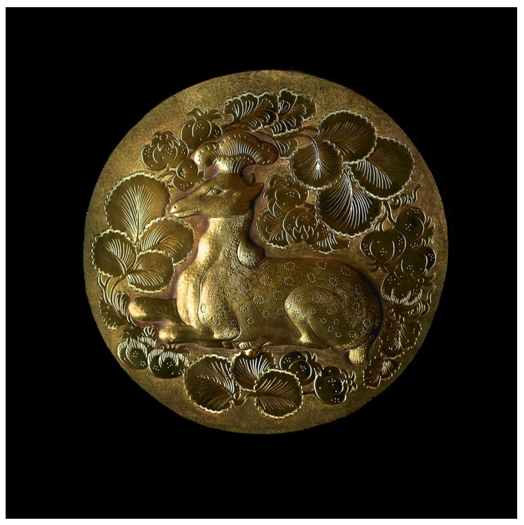


