Climate Change Effects on Carbonation Process: A Scenario-Based Study

Abstract

Using a mathematical model of concrete carbonation that describes the variation in porosity as a consequence of the involved chemical reactions, we both validated and calibrated the related numerical algorithm of degradation. Once calibrated, a simulation algorithm was used as a forecasting tool for predicting the effects on the porosity of concrete exposed to increasing levels of $C{O}_2$ emissions, as well as to rising temperatures. Taking into account future projections of environmental modifications deriving from climate changes, some scenarios were produced numerically by the mathematical algorithm that showed the effects of different pollution levels and global warming on the porosity of Portland cement in a time window of years. Finally, a theoretical study on the effects of pollution levels on the carbonation constant determining the advancement in the carbonation front was carried out for the analyzed scenarios.

1. Introduction

The interactions between environment and building heritage, i.e., monuments, archaeological sites, and historical and modern buildings have always been, and will continue to be, crucial for conservation issues. Moreover, the deterioration and damage of materials caused by weathering processes is still not completely understood since it is a highly complex phenomenon resulting from the interaction of both chemical and mechanical processes.

As natural stones are exposed to the modification of the environment and surrounding landscapes, concrete is also subjected to attack by multiple damaging factors, such as weathering, chemical aggression and abrasion, that may cause its deterioration in terms of a modification of the original form, quality and serviceability. Such weathering processes are always associated with water flow within the material, determined by wetting or infiltration, caused by meteoric precipitation or groundwater capillary rise, respectively.

An increased rate of extreme conditions due to climate change also constitutes a further threat, increasing the decaying rates and contributing to the occurrence of new degradation mechanisms. This happens because climatic changes can not only influence the frequency and intensity of hazardous events but can also worsen the physical, chemical and biological mechanisms causing the degradation of the structure and its materials. In recent years, research communities have started to discuss the impact of climate change on cultural heritage (CH). Since 2003, the number of papers on this subject increased significantly; see [1,2]. The changes in the climate system have been studied by climate scientists; see, for instance, [3,4,5]. In particular, the studies presented by NOAA Climate.gov show that environmental changes in recent decades are leading to a progressive increase in the $C{O}_2$ concentration in the atmosphere, along with human emissions. The Intergovernmental Panel on Climate Change (https://www.ipcc.ch/, accessed on 8 November 2022) takes into account possible scenarios of $C{O}_2$ emissions, showing that, in the near future (up until 2050), the $C{O}_2$ concentration will grow with different rates of increase and, in only a few cases, might be similar to that in 2015.

The environmental changes may affect CH buildings and artifacts due to the synergistic action of atmospheric agents and pollutants; see the recent studies in [6,7]. Such phenomena may determine an irreversible weakening of the mechanical strength and an increased vulnerability to the chemical aggression of porous materials through several mechanisms, such as freeze–thaw cycles, a change in precipitation, corrosion, salt crystallization cycles and an increased frequency of extreme events, just to mention a few; see [8,9,10,11,12,13]. Recently, predictive maintenance, consisting of anticipating future deterioration through appropriate diagnostic techniques, has emerged as a new tool for monitoring and protecting CH sites [14]. Such a diagnosis is carried out by collecting and analyzing, with statistical tools, data on the constitutive materials of the work of art, as well as the action of environmental factors at the CH site. Our approach is within the model-driven framework on predictive maintenance, based on mathematical models for CH (equations describing deterioration processes and the effects of conservation practices)—see, for instance, [15,16,17,18]—coupled with data derived from laboratory experiments and/or gathered by sensors suitably placed at the CH site.

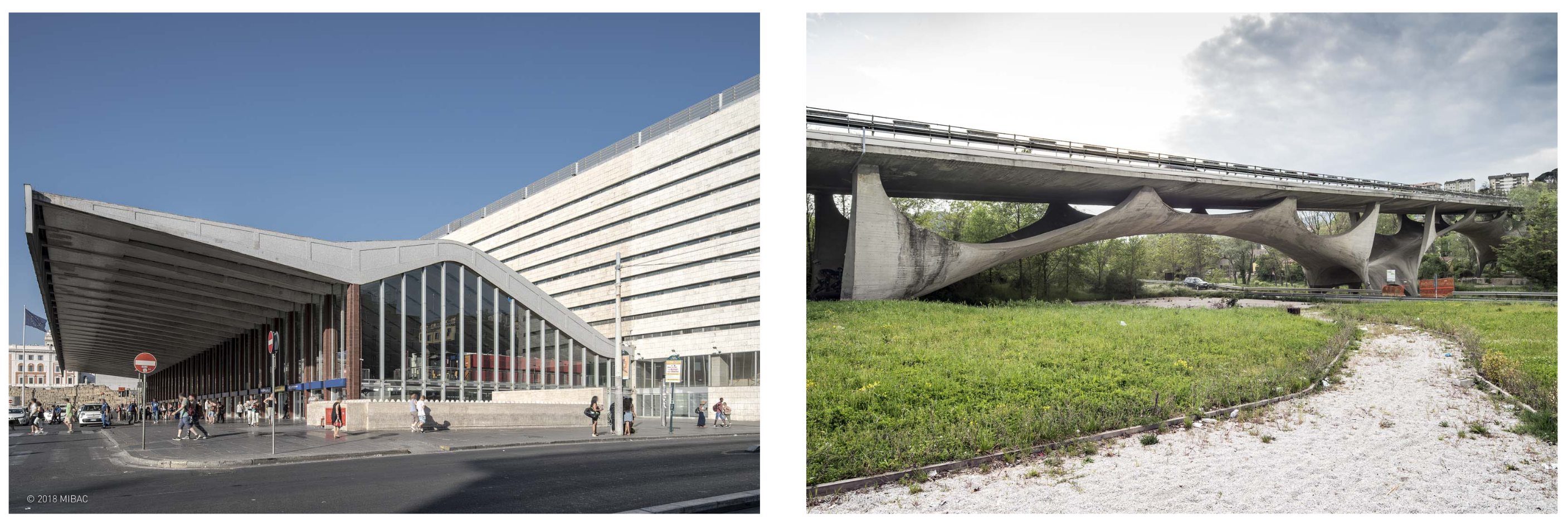
Our study is focused on concrete since it is the most widely used construction material worldwide [19], as it is employed in the construction of buildings, stadiums, stairs, sidewalks and foundations; see Figure 1.

Such a material has a porous structure and its durability is mainly due to its resistance to chemical aggression. In particular, one of the most important degradation phenomena for concrete is carbonation, caused by carbon dioxide in the atmosphere. As shown in Figure 2, environmental changes in recent decades have determined a constant increase in the carbon dioxide concentration in the atmosphere. This fact may accelerate the damage process of building structures.

Concrete carbonation is a complex process whose study requires the cooperation of chemists, engineers and mathematicians in order to capture its features. It is caused by a sequence of chemical reactions that consume calcium hydroxide ($Ca{\left(OH\right)}_2$) and form calcium carbonate ($CaC{O}_3$). The above reactions are induced by carbon dioxide ($C{O}_2$), which is transported by water through the porous medium.

Although concrete is a long-lasting material, its degradation and the consequent weakening may be due to the sulfation of the cementitious matrix, freeze–thaw cycles and the corrosion of steel armor caused by carbonation. Indeed, a basic environment inside the non-carbonated concrete forms a thin film of oxide that protects the steel bars reinforcing the structures, and such a layer is maintained as long as the environment has a pH value of at least 13. In carbonated areas, the presence of carbon dioxide instead neutralizes the alkalinity of concrete with the solution within the pores, assuming a pH value inferior to 9. This causes the destruction of the protective layer and starts corroding the steel bars [20].

In the literature, many experiments for quantitatively evaluating the effects of the carbonation process on cement materials can be found. Since, in natural conditions, the carbonation process is very slow, most of the experiments are carried out in an accelerated regime. For fixed conditions of the $C{O}_2$ concentration, temperature, humidity and time, the samples are subjected to carbonation in a sealed chamber [21]. At the end of the test, the specimens are split, cleaned and sprayed with a phenolphthalein pH indicator, which is an organic compound that is colorless in an acid environment (carbonated part) and turns pink in a basic environment (non-carbonated part); see, for instance, [22,23]. SEM microscope observations and X-rays allow for the quantification of the effect of carbonation by identifying the presence of $CaC{O}_3$ formed and residual $Ca{\left(OH\right)}_2$ not yet reacted with $C{O}_2$. From the comparison of the sample before and after carbonation, the material, initially rich in calcium hydroxide, transforms into being mainly composed of $CaC{O}_3$, clearly indicating that the reaction with $C{O}_2$ has taken place [24,25]. Porosity represents a fundamental parameter for process control that allows us to evaluate the effect of carbonation on the structure of cement. To this aim, gammadensimetry and mercury intrusion analysis can be carried out.

Carbonation has attracted research interests also within the mathematical community and there is a huge amount of literature addressing the mechanism of carbonation with different mathematical models; see, for instance, [26,27,28,29,30,31,32,33,34].

In [35], we introduced a mathematical model describing porosity variation as the result of several intermediate chemical reactions triggered by the penetration of carbon dioxide that diffuses and is transported into the pores by water that is present.

The present paper describes the application of a mathematical model toward the simulation of CH degradation under climate change scenarios. Such scenarios are introduced in Section 2. The mathematical-based simulation algorithm is presented in Section 3. Section 4 is devoted to describe the fitting procedure of the mathematical-based simulation algorithm against laboratory data obtained in natural conditions of the carbon dioxide concentration. Then, in Section 5, we present different pollution scenarios produced by the simulation algorithm with the forecast of porosity variation occurring during the carbonation process. Moreover, a theoretical study on the effects of climate changes in terms of pollution levels on the carbonation constant K was carried out for the analyzed scenarios.

2. Review on Climate Change Scenarios

Given the scope of the paper, a brief discussion of some elements of the global climate crisis is necessary. Since a wide and deep overview on the matter is outside our purposes, we focused on the elements that are relevant for the present research: the carbon dioxide concentration in the atmosphere and global warming. For each of the above elements, a description of the literature sources of climate data that we used in our simulations is provided (see Section 5).

2.1. Atmospheric Pollution: $C{O}_2$ Emission Levels

The Intergovernmental Panel on Climate Change (IPCC)1 is the UN body that advances knowledge of every aspect related to climate change, with a particular emphasis on human-induced climate change. IPCC “prepares comprehensive Assessment Reports about the state of scientific, technical and socio-economic knowledge on climate change, its impacts and future risks, and options for reducing the rate at which climate change is taking place”.

One of the main forces of climate change is the emission of gases due to human activities (such as industry production, transportation, etc.). Among these gases, carbon dioxide has a central role and has become a reference measure of climate change. In its reports, IPCC takes into account several future scenarios of emissions based on assumptions about social, economic and technical development. These shared socio-economic pathways (SSPs) were developed in the year to describe, in a self-consistent logic, major trends of the economy, human lifestyle, technology, demography, policy, etc. There are five SSPs and each provides distinct routes that describe how societies might act in the future and how these actions will impact our environment [36].

SSP1

Sustainability—Taking the Green Road (Low challenges to mitigation and adaptation);

SSP2

Middle of the Road (Medium challenges to mitigation and adaptation);

SSP3

Regional Rivalry–A Rocky Road (High challenges to mitigation and adaptation);

SSP4

Inequality—A Road Divided (Low challenges to mitigation, high challenges to adaptation);

SSP5

Fossil-fueled Development—Taking the Highway (High challenges to mitigation, low challenges to adaptation).

Concerning atmospheric pollution, Figure 3 shows the evolution of the concentration of carbon dioxide in the atmosphere from 2015 to 2150 for several scenarios; see [37]. We can observe that, in the near future (up until 2050), the carbon dioxide concentration keeps increasing under all scenarios; the rate of increase differs for each scenario. However, after at least 2050, some scenarios foresee a slow decrease in concentration; in a few cases, the concentration of carbon dioxide in 2150 will be equal to the concentration in 2015.

In this work, we show some simulations of the carbonation of concrete using the values of carbon dioxide concentration following the scenarios developed in [37]. The actual values of carbon dioxide concentration that we used in our simulations are listed in

Table 1. The values (percentage) of carbon dioxide concentration foreseen for 2075 for the indicated scenarios. Values taken from [37].

SSP1-1.9	SSP4-6.0	SSP5-8.5
0.041973	0.060695	0.080169

.

Remark 1.

The codes of the scenarios in Table 1 are identified by the following rule: SSPx-y.z, where x is the number of the related shared socio-economic pathway and y.z is the target radiative forcing expected by the year 2100. For example, the code SSP4-6.0 is related to SSP4 and foresees a value of radiative forcing of 6.0 W/m² at the end of the century. Radiative forcing is a measure of the imbalance between the incoming solar radiation and the outgoing IR thermal emission due to the change in a variable (i.e., the increase/decrease in carbon dioxide concentration) while all other variables remain the same.

2.2. Global Warming: Changes in Temperatures and Relative Humidity

Climate change also acts on the global temperature, since the amount of water vapor in the atmosphere is changing, which has potentially significant effects. Over the last few decades, global warming has been observed and studied and, correspondingly, climate models have been developed. Climate scientists foresee that the Earth has a high probability to continue to warm over this century and beyond, with a corresponding increase in temperatures [3,4]. Indeed, global warming is caused by the growth in carbon dioxide emissions associated to the presence of other harmful gases produced by human activities. According to a wide range of climate model simulations [38,39], the global average temperature could be between 1.1 and 5.4 °C warmer in 2100; see Figure 4. Such scenarios are the results of projections, but it is also possible that greenhouse gas concentrations may increase at higher rates with respect to those indicated in the graph. In fact, carbon dioxide emissions are increasing at a rate of more than 3% per year; if the rate would maintain the same level, in the future, the carbon dioxide concentration in the atmosphere would exceed the scenario depicted in red by the end of this century or even before.

Regarding the relative humidity, further investigations and studies are still needed to be able to predict its trend in land through the next decades. Indeed, the RH values may be related to many factors, such as changes in atmospheric circulations and land surface properties; see [3].

3. The Mathematical-Based Simulation Algorithm

Here, we refer to the mathematical model recently introduced in [35]. Such a model describes the movement of water (indicated by the letter w) within the porous stones; carbon dioxide (a) dissolved in water; the carbonate ion (b) produced by the dissolution of carbon dioxide; the evolution of calcium hydroxide (i), which reacts with carbonate to produce calcium carbonate; the evolution of calcium carbonate (c), produced by the above reaction and later dissolving; finally, the evolution of calcium ion (e) produced by the dissolution of calcium carbonate. The model will describe the subsequent change in porosity, i.e., the fraction of the volume of voids over the total volume of the porous sample, ($\epsilon$). The complete model reads as follows:

$$\left\{\begin{array}{c}\frac{\partial w}{\partial t}=\frac{\partial }{\partial z}\left({\left(\frac{\epsilon -w_{min}}{{\epsilon }_0-w_{min}}\right)}^{\frac{19}{6}}D(w,\epsilon )\frac{\partial w}{\partial z}\right)+r_w\hfill \\ \frac{\partial \left(wa\right)}{\partial t}=\frac{\partial }{\partial z}\left(a{\left(\frac{\epsilon -w_{min}}{{\epsilon }_0-w_{min}}\right)}^{\frac{19}{6}}D(w,\epsilon )\frac{\partial w}{\partial z}\right)+\frac{\partial }{\partial z}\left(D_{a}w\frac{\partial a}{\partial z}\right)+r_a\hfill \\ \frac{\partial \left(wb\right)}{\partial t}=\frac{\partial }{\partial z}\left(b{\left(\frac{\epsilon -w_{min}}{{\epsilon }_0-w_{min}}\right)}^{\frac{19}{6}}D(w,\epsilon )\frac{\partial w}{\partial z}\right)+\frac{\partial }{\partial z}\left(D_{b}w\frac{\partial b}{\partial z}\right)+r_b\hfill \\ \frac{\partial i}{\partial t}=r_i\hfill \\ \frac{\partial e}{\partial t}=r_e\hfill \\ \frac{c}{m_c}=\frac{i_0}{m_i}+\frac{c_0}{m_c}+\frac{e_0}{m_e}-\frac{i}{m_i}-\frac{e}{m_e}\hfill \\ \epsilon ={\epsilon }_1+({\epsilon }_0-{\epsilon }_1)\frac{i}{i_0}+{\epsilon }_2\left(\frac{e}{e_0}-1\right).\hfill \end{array}\right.$$

(1)

The terms $r_k,k=w,a,b,i,c,e$ represent the chemical reactions, defined according to the following equations:

$$\begin{array}{ccc}\hfill r_w& =& m_w({\omega }_{ib}-{\omega }_a)\hfill \\ \hfill r_a& =& -m_a{\omega }_a\hfill \\ \hfill r_b& =& -m_b({\omega }_{ib}-{\omega }_a-{\omega }_c)\hfill \\ \hfill r_i& =& -m_i{\omega }_{ib}\hfill \\ \hfill r_c& =& m_c({\omega }_{ib}-{\omega }_c)\hfill \\ \hfill r_e& =& m_e{\omega }_c\hfill \end{array}$$

where the terms $m_k,k=w,a,b,i,c,e$ indicate the molar masses of the respective substances, and the ωs describe the single chemical reactions and are defined as follows:

$$\begin{array}{ccc}\hfill {\omega }_a& =& \nu \frac{a}{m_a},\mathrm{dissolution}\mathrm{of}C{O}_2\mathrm{in}\mathrm{water}\hfill \\ \hfill {\omega }_{ib}& =& \mu \left(\frac{i}{m_i}·\frac{b}{m_b}\right),\mathrm{reaction}\mathrm{between}Ca{\left(OH\right)}_2\mathrm{and}CaC{O}_3\hfill \\ \hfill {\omega }_c& =& \delta \frac{c}{m_c},\mathrm{dissolution}\mathrm{of}CaC{O}_3\hfill \end{array}$$

where $\nu$, $\mu$ and $\delta$ are the reaction rates that represent the key parameters of our model, since their values take into account the different time scales of the chemical reactions involved in the carbonation process. In particular, $\nu$ represents the reaction coefficient between carbon dioxide and water, $\mu$ is the reaction coefficient between calcium hydroxide and carbonate ions and $\delta$ is the dissolution rate of calcium carbonate.

Remark 2.

Since porosity varies as a consequence of carbonation, a couple of words are in order to explain how we model it. Porosity changes following two processes:

• Calcium hydroxide reacts with carbonate ions to form calcium carbonate; this process reduces porosity.
• Calcium carbonate dissolves; this process increases porosity.

Following the same arguments as in [35], we can represent porosity with the following expression:

$$\epsilon ={\epsilon }_1+({\epsilon }_0-{\epsilon }_1)\frac{i}{i_0}+{\epsilon }_2\left(\frac{e}{e_0}-1\right),$$

(2)

where:

${\epsilon }_0$

is the porosity of the non-carbonated concrete;

${\epsilon }_1$

is the porosity of (totally) carbonated concrete;

${\epsilon }_2$

represents how porosity varies when calcium carbonate dissolves.

3.1. Initial and Boundary Conditions

The mathematical model is endowed with initial and boundary conditions for the unknown variables. Here, we consider a concrete specimen in the domain $[0,L]$, with $L>0$. The left boundary $z=0$ identifies the surface in contact with the environment, with which the exchange of humidity, carbon dioxide and carbonate occurs. For the unknowns, we impose initial conditions of the form

$$f(z,0)\equiv f_0\mathrm{for}f=w,a,b,c,i,e.$$

Notice that no boundary conditions are needed for the variables i, c and e since these are solutions of ODEs and their evolution in space only depends on the evolution of the other variables. For the unknowns $w,a$ and b, we impose a zero flux condition at the right boundary $z=L$, i.e.,

$$\frac{\partial f}{\partial z}=0\mathrm{for}f=w,a,b.$$

At $z=0$, we assign a Dirichlet condition for water, i.e.,

$$w(0,t)\equiv \overline{w}\left(t\right),$$

where the constant $\overline{w}\left(t\right)$ is the value of the (time-dependent) environmental moisture content computed as

$$\overline{w}=SVD\left(T\left(t\right)\right)RH\left(t\right),$$

(3)

where SVD is the saturated vapor density in [g/cm³] computed as in [27]:

$$SVD\left(T\left(t\right)\right)={10}^{-6}\times (5.018+0.32321T\left(t\right)+8.1847\times {10}^{-3}T{\left(t\right)}^2+3.1243\times {10}^{-4}T{\left(t\right)}^3),$$

(4)

where temperature T and relative humidity $RH$ can be time-dependent if we consider real environmental settings. If instead, we refer to the experimental settings such as those reported in [22], we assume a relative humidity of $RH=70$% and temperature $T=20$ °C.

Then, for a, we assume that the flux at $z=0$ depends on the difference between the internal and external carbon dioxide concentration:

$$\frac{\partial a}{\partial z}(0,t)=-K_a(a(0,t)-\overline{a}\left(t\right)),$$

where $K_a$ is an unknown constant describing the penetration rate of carbon dioxide estimated from the calibration against data and $\overline{a}\left(t\right)$ is the value of the external carbon dioxide concentration.

Remark 3.

Most often, in experimental works, the concentration of carbon dioxide is given as non-dimensional units as a percentage of the substance within the mixture; however, in our settings, we need the value $\overline{a}$ expressed in dimensional units. Given a concentration of carbon dioxide at $y\%$, $\overline{a}$ is computed in g/cm³ as:

$$\overline{a}\left(t\right)=\frac{\frac{m_{a}y}{R{T}_K\left(t\right)}}{{10}^3},$$

(5)

where $T_K\left(t\right)$ is the temperature expressed in Kelvin and $R=0.082Latm{K}^{-1}mo{l}^{-1}$ is the gas constant.

Note that, if we consider laboratory conditions reported in [22], we have the $\overline{w}$ and $\overline{a}$ constant.

We assume the null-flux condition at the left boundary for carbonate:

$$\frac{\partial b}{\partial z}(0,t)=0.$$

The model described above is able to describe the evolution of the carbonation process in the time interval $[0,T]$, with $T>0$.

3.2. Numerical Algorithm

For the simulations, we assumed the model parameters listed in

Table 2. Parameters of the model (1).

	Description	Units	Value	Ref.
h	Specimen’s height	cm	2	datum
$\Delta z$	Space step	cm	0.1	-
$\Delta t$	Time step	s	4	-
A	Shape coefficient of water diffusivity	cm2/s	$3.24\times {10}^{-8}$	[28]
B	Shape coefficient of water diffusivity	-	100	[28]
${\epsilon }_0$	Porosity of the unperturbed material	-	0.2	[41]
${\epsilon }_1$	Porosity after complete consumption of $Ca{\left(OH\right)}_2$	-	0.08	hypothesis/[42]
${\epsilon }_2$	Porosity change due to $CaC{O}_3$ dissolution	-	0.025	hypothesis/[42]
$D_a$	Diffusivity of $C{O}_2$ in water at 20 °C	cm2/s	4.8 $\times {10}^{-3}$	calibrated against data
$D_b$	Diffusivity of $C{O}_3^{2-}$ in water at 20 °C	cm2/s	0.81 $\times {10}^{-5}$	[43]
${\rho }_w$	Density of water	g/cm3	1	[44]
$\nu$	Coefficient of reaction between $C{O}_2$ and water at 20 °C and 1 atm	s−1	1	calibrated against data
$\mu$	Coefficient of reaction between $Ca{\left(OH\right)}_2$ and $C{O}_3^{2-}$ at 20 °C and 1 atm	cm3/(mol s)	$7\times {10}^{-2}$	calibrated against data
$\delta$	Dissolution rate of $CaC{O}_3$ at 20 °C and 1 atm	s−1	$6\times {10}^{-9}$	calibrated against data
$m_a$	Molecular mass of $C{O}_2$	g/mol	44.01	[45]
$m_b$	Molecular mass of $C{O}_3^{2-}$	g/mol	60.01	[45]
$m_c$	Molecular mass of $CaC{O}_3$	g/mol	100.09	[45]
$m_e$	Molecular mass of $C{a}^{2+}$	g/mol	40.08	[45]
$m_i$	Molecular mass of $Ca{\left(OH\right)}_2$	g/mol	74.10	[45]
$m_w$	Molecular mass of water	g/mol	18.01	[45]
$w_0$	Initial water content	g/cm3	0.622	[22]
$a_0$	Initial concentration of $C{O}_2$	-	0.03%	[22]
$b_0$	Initial concentration of $C{O}_3^{2-}$	g/cm3	$1.3\times {10}^{-11}$	hypothesis
$i_0$	Initial concentration of $Ca{\left(OH\right)}_2$	g/cm3	$5.2\times {10}^{-2}$	[22]
$e_0$	Initial concentration of $C{a}^{2+}$	g/cm3	$8.9\times {10}^{-3}$	hypothesis
$c_0$	Initial concentration of $CaC{O}_3$	g/cm3	$9.8\times {10}^{-4}$	[22]
$\overline{w}$	Moisture content of the ambient air for $UR=70\%,T=20 °C$	g/cm3	$0.25$	datum
$\overline{a}$	Concentration of $C{O}_2$ at the boundary	g/cm3	derived with Formula (5) for {0.03%, 0.04%, 0.06%, 0.08%}	scenarios
$K_a$	Penetration rate of $C{O}_2$ in the medium	cm−1	${10}^4$	calibrated against data

.

The interval $[0,L]$ is discretized with a step $\Delta z=\frac{L}{N+2}$, with $\lambda =\frac{\Delta t}{\Delta z},z_j=j\Delta z,j=0,\dots ,N+1$. We also set $w_j^n=w(z_j,t_n)$ as the approximation of the function w at the height $z_j$ and at the time $t_n$.

We can assume that:

$$\begin{array}{c}\hfill V_j^n=D_w{\left(\frac{{\epsilon }_j^n-w_{min}}{{\epsilon }_0-w_{min}}\right)}^{\frac{19}{6}}\frac{w_{j+1}^n-w_{j-1}^n}{2\Delta z},\mathrm{for}j=1,\dots ,N,\end{array}$$

with the boundary values set as follows:

$$\begin{array}{ccc}\hfill V_0^n& =& 0;\hfill \\ \hfill V_{N+1}^n& =& 0.\hfill \end{array}$$

As shown in [35], if we define

$$\begin{array}{c}\hfill {\Delta }_j(u,v):=\frac{(u_j+u_{j+1})(v_{j+1}-v_j)-(u_{j-1}+u_j)(v_j-v_{j-1})}{2\Delta z^2}.\end{array}$$

the numerical algorithm is the following:

$$\begin{array}{cc}\hfill w_j^{n+1}& =w_j^n+\Delta t{D}_w{\Delta }_j\left({\left(\frac{\epsilon -w_{min}}{{\epsilon }_0-w_{min}}\right)}^{\frac{19}{6}},w^n\right)\\ & +\Delta t{m}_w\left(\frac{\mu }{m_i{m}_b}\frac{i_j^{n+1}{b}_j^n+i_j^n{b}_j^{n+1}}{2}-\frac{\nu a_j^n}{m_a}\right),j=1,\dots ,N,\\ \hfill a_j^{n+1}& =\frac{1}{w_j^n+\nu \Delta t}\left\{{\left(wa\right)}_j^n+\Delta t\frac{|V_{j+1}^n|a_{j+1}^n-2|V_j^n|a_j^n+\left|V_{j-1}^n\right|a_{j-1}^n}{2\Delta z}\right.\\ & \left.+\Delta t\frac{V_{j+1}^n{a}_{j+1}^n-V_{j-1}^n{a}_{j-1}^n}{2\Delta z}+\Delta t{D}_a{\Delta }_j(w^n,a^n)\right\},j=1,\dots ,N,\\ \hfill b_j^{n+1}& =\frac{1}{w_j^n+\Delta t\frac{\mu }{2m_i}{i}_j^n}\left\{{\left(wb\right)}_j^n+\Delta t\frac{|V_{j+1}^n|b_{j+1}^n-2|V_j^n|b_j^n+\left|V_{j-1}^n\right|b_{j-1}^n}{2\Delta z}\right.\\ & +\Delta t\frac{V_{j+1}^n{b}_{j+1}^n-V_{j-1}^n{b}_{j-1}^n}{2\Delta z}+\Delta t{D}_b{\Delta }_j(w^n,b^n)\\ & \left.+\Delta t\frac{\nu m_b}{m_a}{a}_j^n+\Delta t\frac{\delta m_b}{m_c}{c}_j^n-\Delta t\frac{\mu }{2m_i}{i}_j^{n+1}{b}_j^n\right\},\\ & j=1,\dots ,N,\\ \hfill i_j^{n+1}& =\frac{1}{1+\frac{\Delta t}{2}\frac{\mu b_j^n}{m_b}}\left\{i_j^n-\frac{\Delta t}{2}\frac{\mu }{m_b}{i}_j^n{b}_j^{n+1}\right\},\\ \hfill e_j^{n+1}& =e_j^n+\Delta t\delta \frac{m_e}{m_c}{c}_j^n,\end{array}$$

$$\begin{array}{cc}\hfill c_j^{n+1}& \hspace{1em}\hspace{1em}\hspace{1em}\hspace{1em}\hspace{1em}\hspace{1em}\hspace{1em}=c_0+m_c\left(\frac{1}{m_i}(i_0-i_j^n)+\frac{1}{m_e}(e_0-e_j^n)\right),\end{array}$$

(6)

$$\begin{array}{cc}\hfill {\epsilon }_j^{n+1}& \hspace{1em}\hspace{1em}\hspace{1em}\hspace{1em}\hspace{1em}\hspace{1em}\hspace{1em}\hspace{1em}\hspace{1em}\hspace{1em}={\epsilon }_1+({\epsilon }_0-{\epsilon }_1)\frac{i_j^n}{i_0}+{\epsilon }_2\left(\frac{e_j^n}{e_0}-1\right),\end{array}$$

(7)

with a suitable discretization of the boundary conditions for w, a and b described above. Note that the scheme above is convergent under the CFL condition $\Delta t\le {\Delta }^{2}z/D_a$. More details are reported in [35].

4. Model Validation and Calibration

In the present section, we show the numerical validation of the mathematical model described above. A fine tuning of key model parameters, i.e., the reaction coefficients $\nu$, $\mu$ and $\delta$, was carried out in a time window of one year in order to represent realistic situations. A common approach usually adopted in order to study the carbonation of concrete is to consider specimens exposed to carbon dioxide concentrations of up to 20%, the so-called accelerated conditions. On the contrary, our aim here was to validate and calibrate the mathematical algorithm over one year for a natural concentration of carbon dioxide in the air, i.e., 0.03%.

In order to validate and calibrate the mathematical model, we referred to data from a carbonation experiment described in [22] performed on a type Portland cement specimen. As described in the work by Pan et al., concrete specimens characterized by a w/c ratio of 0.53 are first polymerized at a temperature of 20 °C and RH of 70% for 24 h; then, they are placed in a seasoning environment at 20 ± 3 °C and 90% RH for 28 days and, successively, samples are placed in a drying oven at 50 °C for 48 h. The carbonation test is executed at T = 20 °C and 70% humidity for $C{O}_2$ concentrations 0.03%, 3% and 20%. In what follows, we considered only the data corresponding to the carbon dioxide concentration of 0.03%. For more details on the experimental setting, the reader may refer to the original paper [22].

In the following numerical tests, we assumed the values of the parameters, taken from the literature or calibrated against data, reported in Table 2.

Since the kinetic coefficients refer to an aqueous solution under ideal conditions, such coefficients were estimated by the simulation algorithm against data, together with the diffusivity coefficient $D_a$. Indeed, in the presence of a significantly lower concentration of $C{O}_2$, we expect that the diffusivity within the material is higher.

In Figure 5, we report the plots of the profiles of the quantities obtained by the mathematical-based algorithm described in Section 3 assuming parameters reported in Table 2. In particular, the left picture shows the system behavior at $t=0$, when the diffusion of gaseous $C{O}_2$ has already taken place in the cement matrix and the carbonic acid formation reaction has just begun, whereas, on the right, the situation at $t=$365 days is depicted.

Looking at the curve profiles of the main quantities involved in the carbonation process and depicted in Figure 5, we obtained a qualitative validation of the model, since it perfectly describes the real phenomenon according to the following aspects:

• Carbon dioxide a (magenta line) enters within the pores and is rapidly consumed;
• Water w (blue line) is consumed by the reaction, as expected;
• The carbonate ion b described by the yellow curve is the sum of two reactions, i.e., the dissolution of carbon dioxide in water and the reaction with calcium hydroxide to form $CaC{O}_3$;
• Calcium hydroxide i shows an “S” shape (green line): near the face in contact with carbon dioxide, calcium hydroxide dissolves by the chemical reaction with carbonate ion; far from there, it is still close to the initial datum since the calcium ion has not yet penetrated sufficiently within the stone;
• On the other hand, the calcium carbonate c (red line) reaches its maximum at the left end of the specimen (in contact with $C{O}_2$) and decreases towards the other end, where the concentration of carbonate ions is very low; moreover, the dissolution of calcium carbonate has already started;
• The calcium ion e (black line), due to the rapid dissolution of calcium hydroxide, only participates in the dissociation reaction of calcium carbonate and it is consequently consumed.

Finally, it is worth noting that, due to the carbonation process, the porosity profile $\epsilon$ (cyan line) depicted in the bottom picture of Figure 5 shows an increasing behavior.

Now, we present the numerical procedure for a fine tuning of model parameters against laboratory data available from the literature. In particular, we used data in ([22], Table 5).

Reporting the concentration of calcium hydroxide and calcium carbonate at the natural exposure of carbon dioxide in the air corresponding to 0.03% for one year. As can be noticed from experimental data, the content of calcium hydroxide always increases with depth, and calcium carbonate shows an opposite trend. Then, a qualitative validation of model outcomes was obtained looking at the relationship between the carbonation depth and the content of calcium hydroxide and calcium carbonate.

In Figure 6, plots of the profiles derived from experimental data (line-circles) taken from [22] for a carbon dioxide concentration of 0.03% and the related numerical results obtained by the model (line-points) using parameters in Table 2 at time $t=365$ days are shown. As can be observed from the left picture in Figure 6, with a fine tuning of model parameters describing reaction rates, not only the qualitative behavior but also the quantitative values of the calcium hydroxide profile are very close to the experimental ones after one year, and the same occurs for the calcium carbonate depicted in the right picture of Figure 6.

In conclusion, a qualitative and quantitative validation of the model is obtained. Indeed, the main feature of our model is its capability to reproduce the mechanism of the creation and consumption of $CaC{O}_3$ on one hand and, on the other hand, the ability to predict the time evolution of the system, even including the long-time behavior.

The forecasting algorithm was implemented in Matlab ⓒ and the computational time taken for a simulation on the complete model with fixed parameters until time $t=365$ days was approximately 2000 s on an Intel(R) Core(TM) i7-3630 QM CPU 2.4 GHz.

5. Mathematical-Based Forecasting Algorithm: Damage Scenarios

5.1. Scenario 1. Laboratory Setting VS. Real Environmental Conditions

In Figure 7, the profiles of the temperature (T) and relative humidity (RH) detected in the laboratory setting (constant values reported in paper [22]) and variable values detected in the environment over a year (2017) by sensors of Arpa Lazio [46] and linearly interpolated on the computational grid are reported. The corresponding boundary conditions for water and carbonic acid obtained by using, respectively, Formulas (3) and (5) are reported in Figure 8.

In Figure 9, the porosity profile in the first point of the material across the time window of $[0,365]$ days is depicted. In particular, we depict the porosity at point $x_0$ computed by the mathematical model (1) at time $T=356$ days for a concentration of carbon dioxide of 0.03% in laboratory (red dotted line) vs. real (blue line) environmental conditions. As can be observed, in both cases, the porosity initially decreases but, after approximately 150 days, it changes its behavior and starts increasing. Moreover, as can be noticed from the superposition between the blue and red curves, the behavior of the porosity obtained by the model (1) using inflow boundary conditions coming from laboratory conditions is reproduces the curves obtained using boundary conditions coming from real environmental conditions quite well. This is probably due to the fact that the inflow of carbon dioxide $\overline{a}$ in the case of constant laboratory conditions is more or less an averaged value of the real values, as can be seen in the right panel of Figure 8.

If we run the simulation algorithm until a time of 5 years, we can see that the porosity still increases, as can be observed in Figure 10, thus possibly determining a weakening of the structure of the building material.

5.2. Scenario 2. Effects of $C{O}_2$ Pollution Growth on Porosity

Here, using the forecasting tool calibrated against laboratory data as described in Section 4, we consider the carbon dioxide concentration scenarios depicted in Figure 3. In particular, we focused on the concentrations of carbon dioxide reported in Table 1 and we simulated the possible scenarios occurring for the porosity profile in these situations; see Figure 11.

As can be seen, in the case of a higher concentration represented by the worst case scenario SSP5-8.5 (approximately 0.08%), the porosity assumes its minimum after approximately 1 month, i.e., approximately three months earlier with respect to the present case, with a 0.03% carbon dioxide concentration. For the intermediate scenarios (SSP4-6.0 and SSP1-1.9), we can observe that the minimum is reached, respectively, after 50 and 80 days.

For longer times, when the porosity starts increasing, all of the curve profiles have the same qualitative and quantitative behavior. This phenomenon should depend on the fact that the porosity growth does not depend on $C{O}_2$ dissolved in water but on the dissolution of calcium carbonate.

A Theoretical Estimate on the Effect of Changes in $C{O}_2$ Levels on the Carbonation Front

When studying carbonation processes, one often evaluates the advancement in the carbonation front (i.e., the boundary separating the carbonated from the non-carbonated zone) in the interior of concrete samples. From an experimental point of view, the carbonated zone can be identified through several techniques, as explained in the introduction. Here, we want to briefly discuss how the carbon dioxide concentration might affect the advancement in the carbonation front.

If we indicate with $\sigma =\sigma \left(t\right)$ the position of the carbonation front, we have that our specimen is divided in two regions:

• Carbonated region $\mathcal{C}\left(t\right)$ defined by $x\in [0,\sigma (t\left)\right]$;
• Uncarbonated region $\mathcal{U}\left(t\right)$, $x\in \left[\sigma \right(t),L]$.

The front moves into the specimen following a square root in time law [47], i.e.,

$$\sigma \left(t\right)=K\sqrt{t}$$

where K ($\mathrm{mm}·{\mathrm{s}}^{-1/2}$) is a constant that depends on the material properties, as well as the concentration of carbon dioxide.

In our previous work [27], we determined the value of K as:

$$K=\sqrt{2{\epsilon }_1\frac{D_a}{1-\omega }\frac{\overline{a}}{{\mu }_h{m}_a}}$$

(8)

where ${\mu }_h$ is the molar density of calcium hydroxide, i.e.,

$${\mu }_h=0.02984\mathrm{mol}·{\mathrm{cm}}^{-3}$$

and $\omega =0.0723$ is a dimensionless parameter taking into account the shrinkage of concrete as an effect of carbonation.

If we insert the values of carbon dioxide for the base case 0.03% in (8), we obtain, after one year, that the front reached the position:

$${\sigma }_{0.03\%}\left(1\mathrm{year}\right)=0.3282\mathrm{cm}.$$

Such a value is smaller than that reported in [22] (i.e., 7.8 mm). However, they reported only one value for the experiments in natural conditions; on the other hand, the value that we obtained here is of the same order of magnitude. Thus, we might assume ${\sigma }_{0.03\%}$(1 year) as a base case to compare the carbonation effect under different pollution scenarios. In other words, here, we evaluated how much the front modifies its position in the three scenarios SSP1-1.9, SSP4-6.0 and SSP5-8.5.

Table 3. The position of the carbonation front (in cm) after one year under the considered climate change scenarios.

	SSP1-1.9	SSP4-6.0	SSP5-8.5
$\sigma$ (1 year)	0.3882	0.4668	0.5365

lists the values of $\sigma \left(t\right)$ after one year using the concentration of carbon dioxide from Table 1.

As one can imagine, since the concentration of carbon dioxide is higher in 2075 than in the present days (according to all three scenarios), the carbonation front penetrates more deeply in concrete stone. It is interesting to see the extent of the penetration with respect to the base case. If we calculate the percentage of increase, i.e.,

$$d\sigma \left(1\mathrm{year}\right)=\frac{\sigma \left(1\mathrm{year}\right)-{\sigma }_{0.03\%} \left(1\mathrm{year}\right)}{{\sigma }_{0.03\%} \left(1\mathrm{year}\right)}·100$$

we can find the values in

Table 4. Percentage of change in front position due to the increased $C{O}_2$ concentration with respect to the base case.

	SSP1-1.9	SSP4-6.0	SSP5-8.5
$d\sigma$ (1 year)	18.2836	42.2381	63.4717

.

For example, in the scenario SSP1-1.9, which foresees a concentration of carbon dioxide that is approximately 40% higher than the base case, the carbonation front increases its depth by “only” 18%.

5.3. Scenario 3. Global Warming Effects on Porosity

The present paragraph is devoted to the numerical study on the influence of the temperature change on the carbonation progress. If we suppose that the RH stays more or less constant and consider a scenario taking into account a temperature increase of 5 °C as predicted in [40], we do not expect to have a significant impact on porosity only depending on this factor. Indeed, as can also be seen in [32], where the authors take into account the effect of the temperature increase in the formulation of the diffusion coefficient, the results show minimal effects (of the order of 1%).

In the next Figure 12, where we depict the porosity profile after 50 days for $C{O}_2$ levels corresponding to the SSP5-8.5 pollution scenario, we can observe that the profiles obtained at a temperature of $T=20$ °C (cyan line) and at $T=$ 25 °C (blue dotted line) are nearly the same.

A Theoretical Study of the Effect of Temperature on Carbonation Front

The mathematical model that we used in this paper does not explicitly describe the action of temperature in carbonation processes. However, we can give some estimate of how temperature affects carbonation in a changing environment. First of all, as we can find in the literature (see for example [32]), we might reformulate the diffusion coefficient through the well-known Arrhenius equation to include temperature, i.e.,

$$D_a\left(T\right)=D_{a}exp\left\{\frac{E}{R}\left(\frac{1}{T_0}-\frac{1}{T}\right)\right\},$$

(9)

where E is the activation energy (40 kJ/mol), R is the gas constant and $T_0$ is a reference temperature (expressed in Kelvin) that we chose here to equal 20 °C. Using the above formula for $D_a\left(T\right)$ and assuming in our settings that the temperature remains constant, the coefficient K in the equation is modified as follows:

$$K\left(T\right)=\sqrt{2{\epsilon }_1\frac{D_a\left(T\right)}{1-\omega }\frac{\overline{a}}{{\mu }_h{m}_a}}.$$

(10)

If we calculate the front $\sigma$ using this new coefficient for a temperature of 25 °C, we find the values in

Table 5. The position of the carbonation front (in cm) after one year under the considered climate change scenarios for a temperature of 25 °C.

	SSP1-1.9	SSP4-6.0	SSP5-8.5
$\sigma$ (1 year)	0.4417	0.5311	0.6104

:

We can see that, after one year, increasing the temperature by 5 °C induces an advancement in the carbonation front by a few tenths of a millimeter.

Thus, temperature does not seems to play a substantial role in carbonation with the considered carbon dioxide concentration. This might seems to contradict other research results, such as in [32]. However, this contradiction is more apparent than real since the authors there considered accelerated conditions (a $20\%$ concentration of $C{O}_2$). Indeed, if we repeat the same calculations above for a concentration of $20\% \mathrm{of} C{O}_2$, we obtain the values in

Table 6. The position of the carbonation front (in cm) after 7 days for a carbon dioxide concentration of 20%.

	20 °C	30 °C
$\sigma \left(t\right)$	1.1734	1.5126

. We can see that, although our model overestimates the position of the front with respect to the values in [32] [Table 13], we can find that the difference is between the two values (approximately $0.34$ cm) and is consistent with the experimental findings.

Thus, we can conclude that temperature does not play a fundamental role in the carbonation processes for “small” concentrations of carbon dioxide.

6. Conclusions

The present paper focused on the forecasting capability of the mathematical model of carbonation - and the related simulation algorithm presented in Section 3. The principal aim of our work was to obtain a reliable simulation algorithm to be used as a numerical forecasting tool for predicting the effects of climate changes (i.e., $C{O}_2$ emission levels, global warming) on the conservation of Portland cement in terms of the porosity variation and penetration depth of the carbonation front.

In this framework, a preliminary qualitative validation of the model followed by a quantitative calibration of its key parameters, i.e., the reaction rates of the chemical reactions involved in the carbonation process, was successfully carried out in Section 4. Indeed, the pictorial representation of the curve profiles of the quantities mainly involved in the carbonation process allows for a first qualitative validation of the model. Then, a quantitative calibration of the model in the case of exposure to a natural carbon dioxide concentration (0.03%) over a year was carried out by comparing laboratory data available from the literature and model outcomes, for both calcium hydroxide and calcium carbonate concentrations, thus resulting in a fine tuning of model parameters. Moreover, a comparison between real vs. controlled laboratory settings was proposed, suggesting no effects in terms of porosity variation. Once calibrated, the simulation algorithm was used as a forecasting tool for predicting damage scenarios in order to evaluate the effects of the possible future increase in the carbon dioxide concentration, as well as in the temperature, as predicted in climate change scenarios reported in Section 2. Finally, since our model does not explicitly describe the advancement in the carbonation front, some theoretical estimates on the effects of climate changes on the penetration of carbon dioxide within cement is proposed in Section 5. In more detail, a study on the effects of climate changes in terms of pollution levels and temperature rise on the carbonation constant K was carried out for the analyzed scenarios, and a substantial agreement with both the experimental and numerical outcomes was obtained.

Then, we can summarize the procedure by the steps reported below:

• A qualitative validation and fine tuning of model parameters against laboratory data;
• A numerical simulation of different damage scenarios quantifying the modification of the front position;
• A theoretical verification of experimental and numerical findings for the analyzed scenarios.

This represents, to our knowledge, the first study on the effects of climate changes on the porosity of Portland cement.

Our future work will follow two interconnected lines of research.

First, we will further enhance the forecasting tool by applying it to different kinds of concrete and with a combination of multiple damaging factors. To this aim, not only data available from literature but ad hoc laboratory experiments and sensor measurements are needed to acquire data (chemical/physical properties such as porosity analyses, gas penetration rates and the presence of other harmful substances). The second line of research will focus on the impact of climate change on CH sites. Indeed, climate change implies modifications in several environmental aspects, such as temperature, precipitation, moisture content, wind intensity, sea level rise and the occurrence of extreme events. All of these changes will affect the degradation mechanisms of monuments or other artifacts in several ways. Thus, we will use our forecasting tool to study how the variation in the above environmental processes impacts cultural assets. This will be interesting from a scientific point of view, as well as for heritage management practice. The final goal of our research in the future is indeed to build a digital-twin prototype of the monitored object in order to develop a mathematical tool for predictive maintenance. Using mathematical algorithms to predict damages from chemical actions and from other mechanisms for building heritage can bring economic savings and allow for the optimal planning of conservative intervention strategies.

References

1. Fatorić, S.; Seekamp, E. Are cultural heritage and resources threatened by climate change? A systematic literature review. Clim. Chang. 2017, 142, 227–254. [Google Scholar] [CrossRef]
2. Orr, S.A.; Richards, J.; Fatorić, S. Climate change and cultural heritage: A systematic literature review (2016–2020). Hist. Environ. Policy Pract. 2021, 12, 434–477. [Google Scholar] [CrossRef]
3. Byrne, M.P.; O’Gorman, P.A. Trends in continental temperature and humidity directly linked to ocean warming. Proc. Natl. Acad. Sci. USA 2018, 115, 4863–4868. [Google Scholar] [CrossRef] [Green Version]
4. Douville, H.; Qasmi, S.; Ribes, A.; Bock, O. Global warming at near-constant tropospheric relative humidity is supported by observations. Commun. Earth Environ. 2022, 3, 237. [Google Scholar] [CrossRef]
5. Pasqui, M.; Di Giuseppe, E. Climate change, future warming, and adaptation in Europe. Anim. Front. 2019, 9, 6–11. [Google Scholar] [CrossRef] [Green Version]
6. Ballard, C.; Baron, N.; Bourgès, A.; Bucher, B.; Cassar, M.; Daire, M.Y.; Daly, C.; Egusquiza, A.; Fatoric, S.; Holtorf, C.; et al. Cultural Heritage and Climate Change: New Challenges and Perspectives for Research. Available online: https://digital.csic.es/bitstream/10261/279867/1/White-Paper-March-2022.pdf (accessed on 8 November 2022).
7. Cassar, J.; Galdies, C.; Muscat Azzopardi, E. A New Approach to Studying Traditional Roof Behaviour in a Changing Climate—A Case Study from the Mediterranean Island of Malta. Heritage 2021, 4, 3543–3571. [Google Scholar] [CrossRef]
8. Doehne, E. Salt weathering: A selective review. Geol. Soc. London Spec. Publ. 2002, 205, 51–64. [Google Scholar] [CrossRef]
9. Scherer, G.W.; Valenza, J. Mechanisms of frost damage. Mater. Sci. Concr. 2005, 7, 209–246. [Google Scholar]
10. Franzoni, E.; Sassoni, E. Correlation between microstructural characteristics and weight loss of natural stones exposed to simulated acid rain. Sci. Total. Environ. 2011, 412, 278–285. [Google Scholar] [CrossRef]
11. Sesana, E.; Gagnon, A.S.; Ciantelli, C.; Cassar, J.; Hughes, J.J. Climate change impacts on cultural heritage: A literature review. Wiley Interdiscip. Rev. Clim. Chang. 2021, 12, e710. [Google Scholar] [CrossRef]
12. Sardella, A.; Palazzi, E.; von Hardenberg, J.; Del Grande, C.; De Nuntiis, P.; Sabbioni, C.; Bonazza, A. Risk mapping for the sustainable protection of cultural heritage in extreme changing environments. Atmosphere 2020, 11, 700. [Google Scholar] [CrossRef]
13. Bonazza, A.; Sardella, A.; Kaiser, A.; Cacciotti, R.; De Nuntiis, P.; Hanus, C.; Maxwell, I.; Drdáckỳ, T.; Drdáckỳ, M. Safeguarding cultural heritage from climate change related hydrometeorological hazards in Central Europe. Int. J. Disaster Risk Reduct. 2021, 63, 102455. [Google Scholar] [CrossRef]
14. Rodrigues, F.; Cotella, V.; Rodrigues, H.; Rocha, E.; Freitas, F.; Matos, R. Application of Deep Learning Approach for the Classification of Buildings’ Degradation State in a BIM Methodology. Appl. Sci. 2022, 12, 7403. [Google Scholar] [CrossRef]
15. Bracciale, M.; Bretti, G.; Broggi, A.; Ceseri, M.; Marrocchi, A.; Natalini, R.; Russo, C. Mathematical modelling of experimental data for crystallization inhibitors. Appl. Math. Model. 2017, 48, 21–38. [Google Scholar] [CrossRef]
16. Giavarini, C.; Santarelli, M.; Natalini, R.; Freddi, F. A non-linear model of sulphation of porous stones: Numerical simulations and preliminary laboratory assessments. J. Cult. Herit. 2008, 9, 14–22. [Google Scholar] [CrossRef]
17. Bretti, G.; Filippo, B.D.; Natalini, R.; Goidanich, S.; Roveri, M.; Toniolo, L. Modelling the effects of protective treatments in porous materials. In Mathematical Modeling in Cultural Heritage; Springer: Berlin/Heidelberg, Germany, 2021; pp. 73–83. [Google Scholar]
18. Saba, M.; Quiñones-Bolaños, E.; López, A.L.B. A review of the mathematical models used for simulation of calcareous stone deterioration in historical buildings. Atmos. Environ. 2018, 180, 156–166. [Google Scholar] [CrossRef]
19. Meyer, C. Concrete as a green building material. In Proceedings of the Construction Materials Mindess Symposium, Vancouver, BC, Canada, 22–24 August 2005; Volume 10. [Google Scholar]
20. Pedeferri, P. Corrosione e Protezione Dei Materiali Metallici. Vol. 1 e 2; Polipress: Milan, Italy, 2010. [Google Scholar]
21. Chang, C.F.; Chen, J.W. The experimental investigation of concrete carbonation depth. Cem. Concr. Res. 2006, 36, 1760–1767. [Google Scholar] [CrossRef]
22. Pan, G.; Shen, Q.; Li, J. Microstructure of cement paste at different carbon dioxide concentrations. Mag. Concr. Res. 2018, 70, 154–162. [Google Scholar] [CrossRef]
23. Villain, G.; Thiery, M. Gammadensimetry: A method to determine drying and carbonation profiles in concrete. Ndt E Int. 2006, 39, 328–337. [Google Scholar] [CrossRef]
24. Thiery, M.; Villain, G.; Dangla, P.; Platret, G. Investigation of the carbonation front shape on cementitious materials: Effects of the chemical kinetics. Cem. Concr. Res. 2007, 37, 1047–1058. [Google Scholar] [CrossRef]
25. Villain, G.; Thiery, M.; Platret, G. Measurement methods of carbonation profiles in concrete: Thermogravimetry, chemical analysis and gammadensimetry. Cem. Concr. Res. 2007, 37, 1182–1192. [Google Scholar] [CrossRef]
26. Ashraf, W. Carbonation of cement-based materials: Challenges and opportunities. Constr. Build. Mater. 2016, 120, 558–570. [Google Scholar] [CrossRef]
27. Bretti, G.; Ceseri, M.; Natalini, R. A moving boundary problem for reaction and diffusion processes in concrete: Carbonation advancement and carbonation shrinkage. Discret. Contin. Dyn. Syst.-S 2022, 15, 2033–2052. [Google Scholar] [CrossRef]
28. Chapwanya, M.; Stockie, J.M.; Liu, W. A model for reactive porous transport during re-wetting of hardened concrete. J. Eng. Math. 2009, 65, 53–73. [Google Scholar] [CrossRef] [Green Version]
29. Chen, T.; Gao, X.; Qin, L. Mathematical modeling of accelerated carbonation curing of Portland cement paste at early age. Cem. Concr. Res. 2019, 120, 187–197. [Google Scholar] [CrossRef]
30. Freddi, F.; Mingazzi, L. Phase-field simulations of cover cracking in corroded RC beams. Procedia Struct. Integr. 2021, 33, 371–384. [Google Scholar] [CrossRef]
31. Kashef-Haghighi, S.; Shao, Y.; Ghoshal, S. Mathematical modeling of CO2 uptake by concrete during accelerated carbonation curing. Cem. Concr. Res. 2015, 67, 1–10. [Google Scholar] [CrossRef]
32. Peng, J.; Tang, H.; Zhang, J.; Cai, S. Numerical simulation on carbonation depth of concrete structures considering time-and temperature-dependent carbonation process. Adv. Mater. Sci. Eng. 2018, 2018, 2326017. [Google Scholar] [CrossRef] [Green Version]
33. Peter, M.A.; Muntean, A.; Meier, S.A.; Böhm, M. Competition of several carbonation reactions in concrete: A parametric study. Cem. Concr. Res. 2008, 38, 1385–1393. [Google Scholar] [CrossRef] [Green Version]
34. Torgal, F.P.; Miraldo, S.; Labrincha, J.; De Brito, J. An overview on concrete carbonation in the context of eco-efficient construction: Evaluation, use of SCMs and/or RAC. Constr. Build. Mater. 2012, 36, 141–150. [Google Scholar] [CrossRef] [Green Version]
35. Bretti, G.; Ceseri, M.; Natalini, R.; Ciacchella, M.C.; Santarelli, M.L.; Tiracorrendo, G. A forecasting model for the porosity variation during the carbonation process. Gem-Int. J. Geomath. 2022, 13, 13. [Google Scholar] [CrossRef]
36. Riahi, K.; Van Vuuren, D.P.; Kriegler, E.; Edmonds, J.; O’neill, B.C.; Fujimori, S.; Bauer, N.; Calvin, K.; Dellink, R.; Fricko, O.; et al. The shared socioeconomic pathways and their energy, land use, and greenhouse gas emissions implications: An overview. Glob. Environ. Chang. 2017, 42, 153–168. [Google Scholar] [CrossRef] [Green Version]
37. Meinshausen, M.; Nicholls, Z.R.; Lewis, J.; Gidden, M.J.; Vogel, E.; Freund, M.; Beyerle, U.; Gessner, C.; Nauels, A.; Bauer, N.; et al. The shared socio-economic pathway (SSP) greenhouse gas concentrations and their extensions to 2500. Geosci. Model Dev. 2020, 13, 3571–3605. [Google Scholar] [CrossRef]
38. Friedlingstein, P.; Houghton, R.A.; Marland, G.; Hackler, J.; Boden, T.A.; Conway, T.J.; Canadell, J.; Raupach, M.; Ciais, P.; Le Quéré, C. Update on CO2 emissions. Nat. Geosci. 2010, 3, 811–812. [Google Scholar] [CrossRef]
39. Solomon, S.; Qin, D.; Manning, M.; Averyt, K.; Marquis, M. Climate Change 2007-the Physical Science Basis: Working Group I Contribution to the Fourth Assessment Report of The IPCC; Cambridge University Press: Cambridge, UK, 2007; Volume 4. [Google Scholar]
40. Climate Change: Global Temperature Projections. Available online: https://www.climate.gov/news-features/understanding-climate/climate-change-global-temperature-projections (accessed on 8 November 2022).
41. Papadakis, V.G.; Vayenas, C.G.; Fardis, M. A reaction engineering approach to the problem of concrete carbonation. AIChE J. 1989, 35, 1639–1650. [Google Scholar] [CrossRef]
42. Alì, G.; Furuholt, V.; Natalini, R.; Torcicollo, I. A mathematical model of sulphite chemical aggression of limestones with high permeability. Part I. Modeling and qualitative analysis. Transp. Porous Media 2007, 69, 109–122. [Google Scholar] [CrossRef]
43. Zeebe, R.E. On the molecular diffusion coefficients of dissolved CO2, HCO3, and CO32− and their dependence on isotopic mass. Geochim. Cosmochim. Acta 2011, 75, 2483–2498. [Google Scholar] [CrossRef]
44. Ball, P. Water—an enduring mystery. Nature 2008, 452, 291–292. [Google Scholar]
45. Shriver, D.; Atkins, P.; Cooper, H. Inorganic Chemistry; Freeman: New York, NY, USA, 1990. [Google Scholar]
46. Arpa Lazio. Available online: https://www.arpalazio.it/web/guest/base-dati. (accessed on 8 November 2022).
47. Leemann, A.; Moro, F. Carbonation of concrete: The role of CO2 concentration, relative humidity and CO2 buffer capacity. Mater. Struct. 2017, 50, 30. [Google Scholar] [CrossRef]
Figure 1. Two examples of concrete buildings. Left Panel: Termini Station in Rome, Italy. Right Panel: Bridge on Basento river in A2 motorway (Italy). Credit: MIBAC, 2018.
Heritage 06 00012 g001
Figure 2. Increasing behavior of carbon dioxide in the atmosphere (blue line) associated to human emissions (gray line) since 1750 (start of the Industrial Revolution) until 2021. Credit: NOAA Climate.gov.
Heritage 06 00012 g002
Figure 3. CO2 concentration scenarios (data taken from [37]).
Heritage 06 00012 g003
Figure 4. Future climate projections based on different human emission pathways. Credit [40]. The picture shows the average of a set of temperature simulations for the 20th century (black line), followed by projected temperatures for the 21st century based on a range of emissions scenarios (colored lines). The shaded areas around each line indicate the statistical spread (one standard deviation) provided by individual model runs.
Heritage 06 00012 g004
Figure 5. Profiles of numerical solutions to the system (1) at time t = 0 (on the left) and after t = 365 days (on the right) obtained with model parameters in Table 2 and with concentration of carbon dioxide of 0.03%. We depict the concentration of water, carbon dioxide, carbonate, calcium hydroxide, calcium carbonate and calcium ion (in g/cm3) and the non-dimensional porosity profile (cyan line). The figures depict the profile on the space dimension (length of the specimen in cm).
Heritage 06 00012 g005
Figure 6. Plots of the profiles derived from experimental data (line-circles) taken from [22] and numerical results obtained by the model (line-points) at time t = 365 days. On the left: profile of measured VS-computed C a ( O H ) 2 and on the right: profile of measured VS-computed C a C O 3 . The y-axis depicts the concentration of the substances (in g/cm3), whereas the x-axis shows the length of the specimen (in cm).
Heritage 06 00012 g006
Figure 7. Temperature and relative humidity in fixed (constant) laboratory conditions vs. interpolated real conditions detected over a year in 2017 in Rome (Arpa Lazio [46]).
Heritage 06 00012 g007
Figure 8. Fixed in laboratory vs. numerical boundary conditions computed with real data for w ¯ and a ¯ using, respectively, Formulas (3) and (5).
Heritage 06 00012 g008
Figure 9. Profile of the porosity at point x 0 computed by the mathematical model (1) at time T = 356 days for a concentration of carbon dioxide of 0.03% in laboratory vs. real environmental conditions.
Heritage 06 00012 g009
Figure 10. Profile of the porosity at point x 0 computed by the mathematical model (1) at time T = 1825 days (5 years) obtained for a concentration of carbon dioxide of 0.03% in laboratory conditions.
Heritage 06 00012 g010
Figure 11. Profile of the porosity at point x 0 computed by the mathematical model (1) at time T = 356 days for a concentration of carbon dioxide of 0.03% (orange line), 0.04% (red dotted line), 0.06% (blue dotted line) and 0.08% (purple dotted line).
Heritage 06 00012 g011
Figure 12. Profile of the porosity at point x 0 computed by the mathematical model (1) at time T = 50 days for a concentration of carbon dioxide of 0.08% at a temperature of T = 20 °C (cyan line) and at T = 25 °C (blue dotted line).
Heritage 06 00012 g012