Article

Working in Tandem to Uncover 3D Artefact Distribution in Archaeological Excavations: Mathematical Interpretation through Positional and Relational Methods

by
Miguel Ángel Dilena
Faculty of Geography and History, Department of Prehistory, Ancient History and Archaeology, Universidad Complutense de Madrid, 28040 Madrid, Spain
Heritage 2024, 7(8), 4472-4499; https://doi.org/10.3390/heritage7080211
Submission received: 10 July 2024 / Revised: 11 August 2024 / Accepted: 13 August 2024 / Published: 18 August 2024

Abstract

:

Featured Application

Here, we propose the integration of network analyses and 3D clustering techniques to comprehensively detect statistical patterns in the artefact spatial distribution of an archaeological site.

Abstract

In recent years, the most advanced pioneering techniques in the computing field have found application in assorted areas. Deep learning approaches, including artificial neural networks (ANNs), have become popular thanks to their ability to draw inferences from intricate and seemingly unconnected datasets. Additionally, 3D clustering techniques manage to associate groups of elements by identifying the specific inherent structures exhibited by such objects based on similarity measures. Generally, the characteristics of archaeological information gathered after extraction operations align with the previously mentioned challenges. Hence, an excavation could be an opportunity to use these prior innovative computing approaches. Our objective is to integrate software techniques to organise recovered artefacts and derive logical conclusions from their spatial location and the correlation between tangible attributes. These results can statistically improve our approach to investigations and provide a mathematical interpretation of archaeological excavations.

1. Introduction

Every archaeological extraction task invariably evolves in a three-dimensional (3D) context. This spatial setting also reveals the positional and descriptive features of the unearthed artefacts and structures. Typically, this type of explorative operation produces extensive but convoluted information that helps decipher the various facets of settlements. However, due to the abundance and complexity of data, a thorough and detailed examination of an excavation becomes demanding, especially when the nature of the sedimentation processes at play blur distinct human occupations in close chronological or spatial proximity.
Present data-mining and deep learning techniques have immense potential for simplifying and untangling such intricacies. In particular, volumetric clustering methods [1,2] and network analysis (NA) approaches [3,4,5] can employ 3D models obtained from the extracted material, which significantly contributes to this clarification purpose. An essential aspect of archaeological excavation involves exploring and interpreting the key events that constitute the site. By implementing such novel strategies, we can arrive at statistically grounded conclusions and provide a plausible mathematical understanding of the newly discovered evidence.
From a data-mining viewpoint, numerous mathematical techniques are available for classifying elements. Archaeology commonly employs density analysis methods that are highly valuable for estimating concentration, particularly in two-dimensional spatial examinations [6,7,8,9,10,11,12,13].
Similarly, density-based clustering approaches [14,15,16,17] scrutinise the volumetric distribution of materials, enabling us to group archaeological components based on their presence or absence, even in three-dimensional spaces (density degree). Such clustering processes can detect spots with varying compactness, recognise object correlations with arbitrary shapes, and identify data points that deviate significantly from the average [18]. Hence, these grouping criteria can capture the character of sedimentation dynamics well, providing an effective technique for associating excavated artefacts in a 3D context. However, they may also exclusively prioritise positional results, disregarding the numerous categorical or qualitative aspects of evidence brought to light that can contribute to classification. Therefore, we can include network analysis during clustering operations to compensate for this shortcoming.
Network analysis is an effective deep learning tool for comprehending the functions and structures of intricate systems [3]. Researchers can use this instrument to discern patterns and trends between entities within a network and understand how these ties impact the system’s overall behaviour. Network analysis often utilises graph theory principles because they offer a potential illustrated interpretation [19]. In this light, several scientific disciplines have already employed graph neural network (GNN) methodologies, as graphs provide a visible and intuitive approach to handling abstract notions such as interactions and relationships. Additionally, graph analysis supplies an inherent foundation for examining connections and resolving complex issues by graphically reducing or converting them into representations that help discover further viewpoints. Researchers have applied such a pioneering technique in unsupervised, semi-supervised, and supervised backgrounds across a vast array of domains such as biology [20,21], chemistry [22], physics [23,24], computer vision [25,26], object detection [27], natural language processing [28,29], traffic networks [30], stock markets [31], text classifications [32], and clustering [33,34], among others. Nevertheless, this approach has been relatively underused in the archaeological domain thus far.
Archaeology has implemented several data-mining (clustering) methods [35,36,37,38] and a few deep learning (GNN) procedures separately, as previously stated, yielding positive results. However, advancements in computational performance, such as memory capacity, calculation speed, and graphical representation, have permitted us to join both pioneering guidelines.
In this study, we integrate both methodologies to examine their disparities and explore their areas of consensus, as well as how they contribute to a more reliable explanation of archaeological evidence based on statistical analysis. Comparing their results may reveal hidden outcomes or validate new proposals, because one strategy is primarily positional-directed while the other approach is rather relational-oriented. Each technique responds to its own point of view; however, by merging the more notable outputs, integration might strengthen the hypotheses of feasible events.
It is worth noting that we exclusively employed three-dimensional heuristics, methodologies, and algorithms during this assessment. Our objective was to perform a thorough analysis considering the 3D spatial parameters of the attributes we studied as observed in their original context.
Aligned with the above, compact and closed spaces, such as confined caves and rock shelters, present potential for excavation methods involving precise and constrained volumetric grid systems to accurately depict 3D excavated areas and their artefacts. Therefore, these environments hold promise as the most suitable locations to apply the innovative three-dimensional procedures we have introduced.
This article emphasises the methodological techniques that allow us to accomplish the previously described goal. Thus, we have chosen a generic case study characterised by an excavation in a Middle Palaeolithic compact rock shelter on the central part of the Iberian Peninsula. It is important to mention that we used only the essential data from this archaeological site, which allowed us to integrate the previous techniques. As a result, we decided to remove any extra content in this paper that did not contribute to employing the methods of such a strategy. To respect this scheme, we provide a concise overview of the practical archaeological topics applicable to our examination and that embrace such an excavation.

1.1. Archaeological Configuration

From a structural standpoint, the Middle Palaeolithic cavity under study had a depositional sequence measuring roughly four and a half metres in height, covering an area of six metres in depth and eleven metres in width.
Furthermore, the examination of the sediments revealed eleven strata, labelled A–K, that were of significant archaeological importance. This circumstance led us to classify such strata into five distinct levels (1–5) based on analysing the lithic and faunal materials found inside them. These levels are described below, from top to bottom [Table 1]:
Henceforth, we will use the term “lithostratigraphic unit” to denote the connection between a certain layer and its corresponding level.
Chronologically speaking, radiocarbon dating with an accelerated mass spectrometer (AMS) and optically stimulated luminescence dating (OSL) show the timeline of the different units in the cavity [39,40] [Table 2].
In general, the animal remains discovered at the rock shelter revealed a variety of incisions, percussion marks, evidence of anthropic flesh removal, notable fragmentation, and the absence of epiphyses and teeth. Moreover, the excavation uncovered numerous formally documented species in the area, including cervids, equids, bovids, canids, and mustelids.
From a lithic perspective, quartz, flint, and jasper were the more abundant materials obtained during the unearthing tasks. These operations also exposed a few retouched fragments, primarily those exhibiting denticulate forms. In addition to unipolar and multipolar reduction lithic processes, the excavation unveiled certain discoidal and Levallois flaking methods [41].

1.2. The Organisation of the Excavation

The excavation activities occurred from 2013 to 2018, which implies that the campaigns employed modern extractive methodologies and detection instruments. We operated a virtually squared grid structure (using plumb lines where possible) to establish the limits of the excavated areas while adhering to the rock shelter’s orientation [Figure 1a]. We implemented this approach to optimise the utilisation of the available space. The sides of each squared component of this grid had a length of one (1) metre.
We used a matrix strategy to locate each element in this grid, representing the west–east limits with letters (E–M) and the north–south limits with numbers (9–13). Therefore, the intersection of one of these letters and numbers uniquely identified a square [Figure 1b]. We internally subdivided these squares into nine (9) smaller squares (3 × 3), roughly 33 cm each, determined by a number from one to nine. We excavated each of these smaller squares at a depth of approximately 3 to 4 cm, depending on the characteristics of the extracted sediment. A numerical identifier indicated the stratum’s depth of this squared parallelepiped inside the excavation, which could vary from 1 to 52 from top to bottom.
Thus, each of these small, squared parallelepipeds ultimately represents the volumetric sector of the excavation. By following this method, each letter (E–M) and its corresponding number (9–13) in the 1-metre square, along with the digit of the internal sub-square (1–9) and the identifier of the depth in question (1–52), uniquely pinpoint a volumetric sector within the extractive operation.
Additionally, we used a total station (Leica TS06, accuracy of 1 mm + 1 ppm) to detect the three-dimensional coordinates of each unearthed artefact’s centroid. Furthermore, we identified an accurately georeferenced point at the beginning of the excavation, located at the vertex of squares L10, L9, K10, and K9 on the limestone roof of the rock shelter. We permanently marked this point with an expansion screw. Similarly, with this TS06, we obtained the ceiling’s Z coordinate for each volumetric sector (i.e., stratum’s depth). The total station provided all the 3D coordinates using the ETRS89/UTM zone 30N reference system (EPSG: 2530) [42]. Such a streamlined approach allowed for trigonometric calculations, effectively correlating all georeferenced artefacts at the archaeological site to a single volumetric sector from which the archaeologists extracted them. Similarly, the univocal sector of belonging served as the sole position reference for all artefacts found during the sieving tasks, as these archaeological elements lacked a precise 3D reference. Finally, each sector was associated with a single lithostratigraphic unit. Consequently, this circumstance also enabled us to identify the specific unit from which each archaeological element originated.

2. Materials and Methods

Reconstructing a mathematical model with a volumetric structure analogous to the excavation process represents the first fundamental step in integrating density clustering methods with network analysis using exclusively three-dimensional heuristics and algorithms.
To implement such a model, we used the same two-dimensional grid network (XY plane) in each archaeological campaign at the site, identifying the 3D coordinates related to the intersection vertices of the 1 m2 squares (plumb lines) and the sub-squares within them (about 33 cm by side). These sub-squares corresponded to the upper faces of the volumetric sectors.
Before beginning the extraction work, we placed all these references in 3D coordinates (EPSG System: 2530). To simplify the computation and focus on the rock shelter, we assumed shifts of A = 900 m, N = 4,534,000 m, and E = 403,900 m. With this constant information, it was possible to excavate in depth (Z axis) and create a stack of a certain number of volumetric sectors (parallelepipeds) with a variable start and an irregular vertical height for each sector face. We compiled such a height using the 3D ceiling’s sector Z coordinate as a vertical start, and the lower next 3D ceiling’s sector Z coordinate as a vertical end of such parallelepipeds. We first stored the Z coordinates in electronic spreadsheets and then converted them into a CSV file [43] for easier maintenance (i.e., the CSV sector file). These data enable a straightforward trigonometric computation of each parallelepiped’s eight vertices [Figure 2a].
At the end of all the campaigns, a complex three-dimensional structure emerged, perfectly adapting to the unearthed cavity and containing a series of ‘bricks’ (parallelepipeds) with homogeneous square surfaces but varying heights. It is worth noting that each parallelepiped is linked to an exclusive lithostratigraphic unit and embraces all the artefacts encountered within it [Figure 2b].
We can formally represent this 3D structure as an array list, where each element of such a data structure represents the 3D coordinate of a vertex in a volumetric sector. Nevertheless, using computational methods, we can also operate the newest graphic technology to depict this spatial representation. We employed the open-source programme Blender (version 3.5.1 macOS) [44] as a support infrastructure to fulfil this objective. Moreover, utilising Blender’s built-in Python framework (version 3.10.9), we managed to automatically duplicate this complex arrangement of parallelepipeds (volumetric sectors), reproduce its geographic reference in 3D space, and finally visually define each lithostratigraphic unit [Figure 3a].

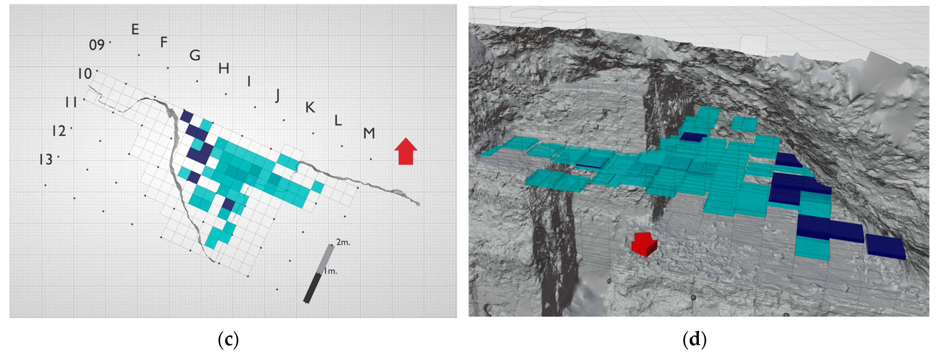
2.1. Artefact Georeferencing

Using the abovementioned EPSG system, we georeferenced all the artefacts we detected in the sediments throughout the excavation [Figure 3b] [45]. We excavated 4190 artefacts in total. We georeferenced 1337 (31.9%) archaeological elements. However, the remaining 2853 (68.1%) components resulting from the sieving process did not have precise three-dimensional coordinates. Instead, such evidence was only associated with the volumetric sector in which we encountered it. This last group typically consisted of tiny archaeological fragments not visible to the archaeologist during excavation operations.
We had to assign a coherent coordinate to integrate these sieved elements into our study. We accomplished this by employing an algorithm that randomly placed such artefacts within their parallelepiped of belonging (volumetric sector). To carry out this calculation, we trigonometrically extracted each parallelepiped centroid. With such a barycentre, we obtained random values of x, y, and z for each unreferenced sieved artefact without leaving the parallelepiped’s perimeter and consequently positioned the object at that coordinate.

2.2. Quantitative and Qualitative Variables

Thus, when we georeference an extracted artefact, we typically determine the centroid’s position in three-dimensional space and assign a coordinate based on a spatial reference system (e.g., EPSG: 2530). An invariable relationship between two distinct archaeological elements in an excavation is quantitative. In this scenario, we can express this relationship numerically using the Euclidean distance (1) between the 3D coordinate of the first artefact’s centroid i and the 3D coordinate of the second artefact’s centroid j by utilising the following formula:
d i j = k = 1 p x i k x j k 2 1 2 ,   w h e r e   p = 3
On the other hand, other types of relationships, this time qualitative, exist between two different archaeological elements that compare their physical traits. These relationships define the discrepancy between two findings (i and j) regarding their tangible attributes.
In Middle Palaeolithic excavations, we find almost exclusively two classes of evidence: lithic and faunal. Some of the previously mentioned qualitative characteristics belong only to the lithic findings category [Table 3], others solely to the faunal remains [Table 4], and the rest to both kinds of evidence [Table 5]. These tables do not consider unattainable values or absence as a category. In our case study, we thoroughly examined and recorded the following substantial features, each with qualitative values:
Utilising both quantitative and qualitative variables is critical in determining whether two elements are comparable or dissimilar in terms of their location and physical characteristics. Hence, such references may help us identify connections that allow us to spatially group these elements and discover associations in their concrete attributes. Consequentially, for each artefact, we also integrated these quantitative and qualitative features into a CSV file (e.g., the CSV artefacts’ attributes file).

2.3. Clustering Process

Cluster analysis is a significant method for database mining. We used clustering to group related information by measuring the distance, similarity, and closeness of data points (specifically artefacts, in this context) for each sample. Although clustering is an unsupervised process because there is no previous information about the number of classified groups or their concrete definition, we can use clustering tendency assessment techniques to determine whether a given dataset contains significant information to make such clustering associations. These assessment methods employ statistical computations to validate the groups. As a result, the present study used the following clustering tendency assessment tests for all archaeological examinations:
  • Hopkins indicator [46]: This determines the presence or absence of spatial data randomization. As the value of this statistical indicator approaches unity, datasets may exhibit clusterability
  • Silhouette technique [47]: This evaluates the quality of the associations in a dataset. An exceptionally high average silhouette extent signifies a meaningful level of clustering [Figure S1]2.
  • Elbow approach [48]: This algorithm considers the overall within-sum squares (WSS). It selects k groups so that including an additional association does not enhance the WSS. In general, the location of an elbow in the diagram represents a reliable indicator of the optimal number of clusters (k) [Figure S2].
  • Visual Assessment of Cluster Tendency (VAT) [49]: This algorithm generates an ordered dissimilarity matrix (ODM) using the Euclidean distance measure. The dissimilarity value among observations directly relates to the degree of colour in such a matrix [Figure S5].
  • Calinski-Harabasz index [50]: This signifies the degree of similarity between an entity and its cluster (cohesion) compared to other associated groups of entities (separation). It endeavours to determine the optimal quantity of clusters (k).
  • GAP index [51]: This statistical index compares the overall variance within clusters for various values of k with their predicted values [Figure S3].
  • Hubert index [52]: This outlines graphical techniques for calculating the value of k. By plotting this marker, we aim to identify a prominent inflexion point corresponding to a substantial and meaningful rise in value [Figure S4].
  • Duda-Hart test [53]: This involves statistical analysis. A p-value of 0 indicates the need for further division of the cluster.
Moreover, clustering analysis includes a variety of techniques for incorporating observations into bunches or conglomerations based on one or more variables. Clustering algorithms aim to group a dataset’s objects into a set of meaningful subclasses founded on such variables.
We decided to employ density-based clustering techniques, which identify clusters separated by low-density regions in high-density areas. Such an approach enables the detection of associations of various physical shapes, as well as the identification of outliers that are compatible with the deposition process at an archaeological site. The crucial idea of density-based clustering is that for each object in a cluster, the neighbourhood of a given radius (ε) has to include a minimum number of elements (minPts) [18].
Some specific algorithms use density-based clustering as a methodology. We used four of these algorithms throughout the current study, including clustering direction centrality (CDC), density-based spatial clustering of applications with noise (DBSCAN), hierarchical density-based spatial clustering of applications with noise (HDBSCAN), a hybrid of DBSCAN and hierarchical clustering, and lastly, ordering points to identify clustering structure (OPTICS) [Table 6].
Statistical researchers have already coded all these clustering approaches using the open-source software R. We employed this framework to proceed with the excavation clustering calculations in R (version 4.3.1 macOS) [54] and R Studio (v. 2023.06.1+524 macOS) [55].
We investigated associations between artefacts from the entire excavation using each of the preceding clustering techniques, relying solely on Euclidean distances (1) without evaluating the significance of the categorical variables.
During this analysis stage, we made a general assumption that encompassed both faunal and lithic artefacts equally. We then applied the previously mentioned procedures individually to the items found at each of the five archaeological levels using the same criteria.
Next, we proceeded with a comprehensive examination of each level and the entire excavation, employing the same clustering methodologies. However, in this instance, we distinguished the artefacts into three categories: faunal, lithic, and thermo-altered. Accordingly, we also tried to find groups based on their categorical variable. Since we can pinpoint the precise lithostratigraphic unit to which the element in the calculated cluster belongs, we can include this unit as helpful information in the results.
Throughout the operations described above, we tested each of the algorithms [Table 6], first with a dataset of only georeferenced elements, and then with a complete dataset (georeferenced and sieved elements). Each time, we randomly regenerated the positioning of the sieved elements within the volumetric sector, following the criteria outlined in previous paragraphs.

2.4. Multiple Factor Analysis (MFA)

As we have seen, an excavation’s outcome entails several quantitative and qualitative variables. For this reason, it is critical for this study to find a method that analyses all artefacts, identifies the groups of dimensional and categorical variables involved, and primarily determines the contribution that these variables can make to the examination.
The factorial method, known as multiple factor analysis (MFA) [56], is a multivariate technique that examines, summarises, and visualises tables where a set of variables describes a group of elements. Multiple sets of attributes, both quantitative and qualitative, organise and define such collections.
Thus, MFA is a combination of principal component analysis (PCA) for quantitative tables [57] and multiple correspondence analysis (MCA) for qualitative tables [58].
MFA examination comprehensively depicts the observations and the interconnections among the variable groups. Consequently, MFA enables us to streamline a group of intricate variables by employing statistical methods to investigate the fundamental dimensions that elucidate the connections among such variables.
We conducted this part of the study using MFA, combining the 3D coordinates (a quantitative finding trait) with the categorical variables (qualitative traits closely examined during the examination process) [Table 3, Table 4 and Table 5] for each artefact (both lithic and faunal). In addition, we evaluated such variables by analysing the five archaeological levels and the entire excavation. Our goal was to determine each variable’s statistical contributions to the site, individually and collectively.

2.5. Graph Neural Network (GNN)

Past archaeological studies have focused on analysing the spatial distribution of artefacts encountered in excavations [6,7,8,9,10,11,12,13]. These types of research conduct density examinations using a variety of positional methods, focusing primarily on how an artefact fits in space compared to other findings. In fact, one of these techniques is 3D density clustering analysis, which we considered above.
However, there is another innovative approach, this time relational in nature through network analysis, specifically the so-called graph neural network (GNN), which offers an alternative viewpoint, aiming to establish, identify, and accentuate the visual relationships between two descriptive variables (nodes) via connections (edges). In practice, these two components (nodes and edges) form a graph (e.g., GNN diagrams [Table 9]).
A graph can be considered a mathematical and visual formalism for representing binary correspondences within a collection of elements. In this case, graph nodes, symbolised as dots, can characterise qualitative values within a spatial dataset. So, for this study, the graph nodes denote every artefact’s categorical attribute, analogously to the MFA method. Graph edges, depicted as lines, define conditional connections between these values [19,59]. The width of the lines and dots can convey details such as the solidity of the contacts between elements or the frequency of their presence. In this case, the GNN uses an unsupervised learning process to identify the correlations among these values uncovered during the extraction of each artefact.
We conducted various computational cycles to perform this calculation, which involved binary-comparing two (r) distinct components of the eleven qualitative variables (n) repeatedly until we exhausted all potential statistical combinations for assessment (2). In mathematical terms, this is expressed as follows:
C n , r = n ! r ! n r !   ;   w h e r e   n = 11   a n d   r = 2 ,   C = 55
Hence, we explored eleven (n) categorical variables and their combinations. For each variable, we scrutinised a different set of individual values [Table 3, Table 4 and Table 5]. We also analysed the eleven lithostratigraphic units (l) accompanying each set of individual values [Table 1]. As a result, the comparisons grew as the units under examination, the categorical variables, and the individual values of these variables increased. Against this background, we accomplished m = 43,692 distinct calculations. Equation (3) represents such a quantity of computations where xi represents the number of individual values that exist in the ith categorical variable (x):
m = l 2 i = 1 n j = 1 n x i x j ,   i f   i j = l 2 i = 1 n x i 2 i = 1 n x i 2 ;   w h e r e   n = 11 , l = 11 , m = 43962
The division into two denotes the combination’s symmetry (the adjacency matrix).
In each confrontation, the computation extracted all artefacts with at least one of the two contrast values as an attribute by level and lithostratigraphic unit. We mathematically (4) obtained the union of these two sets of samples to determine the total number of elements with these characteristics in each level, each lithostratigraphic unit, and the entire excavation.
A     B = A + B A B
For each of these artefacts, we know the volumetric sector to which they belong. Using this information, we extracted only the common parallelepipeds that shared the two qualitative values simultaneously. Thus, we employed these shared areas to find the algebraic total of archaeological elements coinciding volumetrically at that level and in each lithostratigraphic unit of that level, sharing the features under comparison. We divided this sum by the previously calculated union of the two sets of samples at that level and in each unit of that level (4). Thus, it was possible to develop a numerical ratio (percentage) (p) of artefacts that coincided spatially under the attributes analysed (two qualitative individual values, u and v) by level and unit.
We also employed R to write a descriptive and statistical interpretation of these confrontations in English (e.g., [Figure S23]). Additionally, we utilised bar graphs to illustrate these percentages for each comparison across the various lithostratigraphic units (e.g., [Figure S22]).
Furthermore, we know the volume of each spatial sector. Consequently, we can calculate the cubic metres of the lithostratigraphic unit that embraces it and the total volumetric value occupied by the entire excavation (total volume: 16,651 m3) [Figure S26]. Knowing the volumetric proportions of the levels and units in the excavation [Table 7] and the total number of elements that share these two attributes in the whole site, we can infer whether the calculation made at each level and each unit is relevant and statistically significant. According to this criterion, we dismissed the comparisons that were not representative.
With these details, we can also establish a threshold by parametrically determining the minimum percentage of volumetric sectors shared by the two qualitative individual values under consideration (u, v). This threshold allows us to focus on the most notable contributions and vary them as we request to increase or decrease them. By using such adjustable increments or decrements, we can observe how the attributes’ relational contributions evolve in space. This situation permits us to identify which traits may remain stable during the threshold variation and which may emerge gradually.
In such a scenario, we can construct a weighted undirected symmetric adjacency matrix for each level and each lithostratigraphic unit, where the columns and rows represent the s individual qualitative values under examination and the intersection elements mirror the previously calculated numerical ratio (percentage) (p). Thus, the adjacency matrix of this graph representation G = (V, E) [V = vertex, E = edge] is the s × s matrix A, indexed by V, whose (u, v)-entry and (v, u)-entry are defined as follows:
A u v = A v u = p n u m e r i c a l   r a t i o   % ,   i f   u v   E 0   ( % ) ,                                                                 ,   i f   u v     E
Hence, we can describe such graphs as node-weight adjacency matrices in network terms. These data show how often (ratio percentage, p) qualitative values (u, v) appear close to each other in the volumetric space of the level or lithostratigraphic unit (if there is a relation between them).
We constructed the network graph for each level or unit using the tidygraph R package [60]. In network analysis, we can include two tables for undirected graphs. Such tables provide information about the type and size of nodes and edges. Defining the node table entails using the appearance frequencies of each qualitative individual value in the adjacency matrix (the sum of the percentages in that variable’s column or row).
In other words, we sum the values of the neighbouring nodes over all edges in an undirected network (symmetric adjacency matrix) (6).
f u = i = 1 s A u i = i = 1 s A i v ,   i f   u = v
Additionally, we can attach the qualitative attribute (one of the eleven categorical variables) as a column to which the individual value (u or v) belongs.
On the other hand, to determine the edge table, we employ the ratio percentages (p) between the two qualitative variables in the adjacency matrix. Therefore, the adjacency matrix captures the edges between nodes for any given graph structure. We use these edges to determine the distribution of co-occurring neighbour pairs. With these calculations, we can determine that the thickness of the edge lines indicates the strength of the correlation between one individual value and another. Instead, the node’s size indicates the level of involvement of that variable within the level or unit [61].
Furthermore, R software allows us to display these interconnections on an electronic spreadsheet table to order the results based on different values (e.g., lithostratigraphic unit, categorical variable, individual qualitative value, and so on).
During the preceding activities, we tested each algorithm using two datasets: one consisting solely of georeferenced elements and another consisting of both georeferenced and sieved components. We randomly generated the location of the sieved elements within the volumetric sector, adhering to the criteria described in earlier sections.
By utilising network analysis, not only can we visualise the inter-relationships corresponding to each level or unit, but we can also examine and extract specific statistics about them that provide insight into their structural properties. Hence, we can explore the degree of centrality, central nodes, betweenness centrality, and closeness attributes relative to each level or unit [59].

3. Results

So, the methodological process we have examined here yielded two main results. We primarily develop the first outcome in a positional setting based on the various volumetric densities of artefacts found during sediment extraction (3D clustering).
The spatial associations between the categorical attributes of the artefacts we encountered serve as the foundation for the second development, which emerged in a connectivity context (network analysis). We illustrate both results in the following paragraphs.

3.1. Clustering Results

First, we verified that the artefacts discovered during the excavation tasks were clusterable in every level and lithostratigraphic unit based on the clustering tendency assessment techniques [Figures S1–S5]. Second, we confirmed that density-based clustering algorithms can accurately capture the volumetric concentrations naturally formed by the artefacts and their sedimentation processes. Third, we compared the results of all these methods [Table 6], and the OPTICS approach produced the best outcomes for most of the clustering tendency assessment calculations due to its ability to regulate according to a non-mandatory threshold [Figures S6–S12]. From here on, we chose to display the results based on this last criterion because it can handle such statistical flexibility.
That being said, as a first step, we utilised Euclidean distances (1) and the OPTICS methodology to analyse the entire excavation area without considering levels or lithostratigraphic unit separations [Figure 4].
Such examination allowed us to identify at least one archaeological group at levels 2 and 3 [cyan/red]. However, we needed to clarify whether this correlation represented a single, united cluster or two distinct entities, one at each level. In addition, we detected a minimum of three different density groups at level 5 [purple/yellow/dark blue]. The outlier elements are coloured white. Using only the georeferenced artefacts dataset, we found almost the same situation, with the difference that we detected only two clusters at level 5 and not three, covering nearly the same volume.
Subsequently, we again conducted another density-based examination utilising OPTICS, this time considering each level individually and the Euclidean distances (1). Upon further scrutiny, we discovered that level 1 did not generate any artefact groups, level 2 included at least one cluster of components (maybe two) [orange/yellow], and level 3 yielded a minimum of one cluster (perhaps two) [dark blue/cyan]. Once again, level 4 demonstrated its archaeological sterility, and at level 5, we encountered a minimum of three distinct groups [green/magenta/red] [Figure 5 and Figures S6–S12].
The situation was almost identical when we exclusively employed the georeferenced artefact dataset. The only difference was that we identified only two clusters at level 5, rather than three, which occupied a nearly similar volume.
By employing OPTICS clustering techniques once more with the Euclidean distances for each level, we continued grouping without taking into account the categorical variables, but solely the three types of evidence characteristic of this rock shelter: thermo-alterations, lithic industry, and faunal remains [Table 3, Table 4 and Table 5].
At level 3, we observed a substantial collection of thermally modified objects (units 3F and 3G).
After analysing the evidence of lithic industry, we discovered a significant cluster in levels 2 and 3, particularly in the 2D, 3E, and 3G units. Such a considerable group may embrace two separate associations. In addition, we unveiled another prominent assemblage at level 5. Nonetheless, this level may provide at least two more regions where significant concentrations of stone tool remnants could form.
Regarding animal remains, we identified a substantial collection at level 3 and a minimum of three distinct associations at level 5.
The situation was nearly identical when we exclusively employed the georeferenced artefacts dataset. The only distinction was that we identified only two clusters at level 5 rather than three.
Additionally, when using the complete dataset (georeferenced + sieved), we observed that randomly repositioning the sieved artefacts did not affect the clustering results.
Finally, we again used the Euclidean distances (1) and the OPTICS technique to identify clusters, this time related to each categorical variable by level (e.g., Figures S13–S16). Through this examination, we discerned several characteristics. The following percentages represent the proportionate rates of each component within a given category across the whole excavation.
Our inspections indicate that 96.1% of the artefacts at the site did not exhibit any signs of heat treatment. However, in units 3F and 3G, we observed a concentration of black-coloured alterations on animal bones, accounting for 2.9% of the total.
The non-cortex lithic industry was quite prevalent (73.6%) in the excavation. However, we discovered several flint artefacts entirely built by cortex material, accounting for 6.4% of the total evidence found in units 3E and 5K.
Regarding lithic volumes, we identified residual debitage fragments or debris (11%) and cores (2.2%) at level 2 and unit 3E. In addition, we discovered further categories of volumes at levels 3 and 5, which consisted of the following dimensions: 30 mm3 < x < 700 mm3 (34%), 1200 mm3 < x < 5000 mm3 (22.5%), and 5000 mm3 < x < 20,000 mm3 (11.2%). At level 5, we discovered a group that fit within the range of 700 mm3 < x < 1200 mm3 (9.7%).
The examination of the lithic material indicated the presence of brown jasper (17.3%), white quartz (13.7%), honey-coloured Otero flint (7%), and grey Otero flint (4.7%) at levels 3 and 5. At level 3, we discovered grey flint with a composition of 6.7%. In addition, we identified brown Otero flint at a percentage of 8.8% in level 5.
During our analysis at levels 3 and 5, we observed that the most common type of lithic flaking had a flat butt with an indeterminate dorsal and various bulb pronunciations (19.6%). Likewise, we noted a 4.4% occurrence of the lithic industry findings lacking bulbs and butts at these identical levels. Throughout the excavation, we also discovered that the non-retouched lithic industry artefacts represented the majority category (96.9%).
The analysis revealed animal remains of different sizes, including small (6.6%) and big (4.9%) specimens, primarily at levels 3 and 5. In addition, it identified traces of carnivorous animals (Canis lupus, 4.1%) at level 5, as well as remains of the Equus genus (1.2%) at levels 3 and 5.
Similarly, the research detected percussion marks at a frequency of 3.8% at level 3 and trampling indicators at a frequency of 5.6% at levels 3 and 5. Regarding the faunal fractures, we predominantly observed the fresh/fresh rupture type at level 5, with lesser occurrences noted in units 3F and 3G.
In terms of anatomical components, we located clusters of ribs at level 3, accounting for 5% of the total, and teeth at level 5, accounting for 3.6% of the total. Concerning the faunal age [Figures S13–S16], most of the remains (60%) were from adult individuals, primarily found in units 3F and 3G. Nevertheless, we also noticed a more limited group at level 5. We discovered a compact assembly of senile faunal remnants (3.5%) mostly found at level 5.
It is worth noting that the 3D reconstruction of the excavation allows for the direct observation of all the archaeological components, unearthed artefacts, and their respective mathematical clusters, including outlier values. Such visualisation is feasible because the cluster algorithms determine the correspondence between the associations and the elements to which they belong. As a result, the Blender framework [44] can position the resulting grouped assemblages precisely in space within the three-dimensional simulated cavity [Figures S13–S16].

3.2. Multiple Factor Analysis (MFA) Results

MFA is an effective method for simplifying intricate data, uncovering hidden patterns, and laying the groundwork for further in-depth and targeted research. We commonly employ it when analysing multiple interconnected variables, with the aim of comprehending the fundamental structure or patterns within data.
Employing multiple factor analysis (MFA) proved that certain groups of variables significantly affect how statistical contributions of artefacts are defined within an excavation. As we verified above, the clustering procedure identified a similar situation.
We used MFA to determine how much each category and variable contributed to the principal components. We utilised both quantitative and qualitative elements for the faunal, lithic, and thermo-altered elements connected to them [Figures S17 and S20]. Instead, we used Dim1–Dim2 scatterplots for the individual variables of qualitative attributes only [Figures S18, S19 and S21]. We analysed the entire excavation and then delved deeper into each lithostratigraphic unit of interest. Table 8 presents the results in decreasing order.

3.3. Network Analysis (GNN) Results

The analytical methodology using graph neural networks (GNNs) yielded numerical results comparable to those previously evaluated. To observe the progression of the interconnections, we examined the links using two distinct thresholds (46% and 40%). Each threshold denotes the bare-minimum proportion (%) of artefacts shared by two categorical values within the excavation sectors. By incorporating multiple thresholds into the analysis, we can identify the most significant contributions of specific qualitative attributes at each level and unit (for space reasons, the correlations column only describes the results for the 46% threshold option). This investigation yielded the following notable findings, calculated through R [54] (Table 9):
The network analysis provides different measures we can apply to each level and unit for every threshold [Table 10 and Table 11].
The most straightforward metric for assessing node connectivity is degree centrality, which computes an importance score based on the number of connections each node maintains. Betweenness centrality measures how frequently a node finds itself on the shortest path connecting other nodes. Closeness centrality assigns a value to each node, measuring its degree of proximity to all other nodes in the network [3].
Moreover, with the 46% threshold, we obtained 134 connections; with the 40% threshold, we achieved 205 connections in all units. Since the maximum number of connections with the analysed categorical values is 43,962, the first threshold establishes 0.3% of this total, while the second threshold is 0.47% [Table 9].
We found a remarkably similar situation during the ANN examination using only the georeferenced artefact dataset. The ANN only considers attainable categorical values that have a significant qualitative identification. Because of their physical dimensions, most of the sieved artefacts may not have displayed such characteristics during the laboratory analysis.
Furthermore, when using the entire dataset (georeferenced and sieved), we noticed that randomly relocating the sieved artefacts did not affect the networking results.
With the data obtained, we can calculate another helpful statistical index for each unit: the archaeological volumetric density. We estimate this density by dividing the number of artefacts [Table 9] [Figures S24 and S25] by the volume of the lithostratigraphic unit [Table 7] [Figure S26]. The following bar diagram illustrates this statistical element [Figure 6]:

4. Discussion

In this paper, we have conducted a purely 3D spatial analysis to examine the distribution of artefacts and their associations in a rock shelter. We chose the artefacts’ 3D coordinates and eleven categorical variables [Table 3, Table 4 and Table 5] because we had exhaustive information about them. However, it is important to note that we did not obtain complete access to the information about level 3, as the analysis did not consider a few categorical values related to the lithic industry. Researchers are currently working on an analysis to achieve this goal. This limitation in scope may lead to potential statistical biases in this area, especially because, at that level, we discovered the highest volumetric density of artefacts from the excavation [Figure 6]. Nevertheless, we worked with the entire amount of data in our possession.
It is worth mentioning that relying on precise 3D coordinates for artefact georeferencing means that any inaccuracies in data collection could significantly impact the results. Every data position has an associated uncertainty, which must be considered when interpreting spatial data. The rock shelter’s original geological configuration necessitated excavating the cavity from top to bottom. Initially, the narrow gap at the upper levels made it difficult to determine the artefacts’ positions at those strata accurately and to precisely place the total station (TS) to collect them. Fortunately, those levels were almost archaeologically sterile. The TS’s unprecise alignment with the permanent screwed point inside the rock shelter, the lack of suitable light, the prism position during the measure operation, a non-optimal distance or angle range, the operator’s vision, the atmospheric conditions, and the device’s precision itself could all affect the measurement’s accuracy.
Nevertheless, due to the excavation’s organised virtual squared grid structure, we quickly confirmed the consistency of the measurements obtained within each parallelepiped. In both techniques mentioned, each volumetric sector plays a crucial role in comparing the elements inside it. Therefore, these volumetric sectors (parallelepipeds) establish a spatial framework for containment and comparison, and also outline the smaller georeferenced structure (brick) that facilitates the digital reconstruction of the entire excavation, including its levels and units. Such structural organisation provides solidity and reliability to the calculations.
Here, we chose a generic case study. However, we can apply and replicate this approach not only to rock shelters and Palaeolithic spots, but also to other archaeological sites, provided they adhere to volumetric sectors’ organisational excavation criteria. The more confined these blocks are, the more correlations and details we can accomplish and the more precise we can be.
Our primary goal is to demonstrate the methodology used to conduct the exams shown here. Against this background, we have decided to approach the problem from two points of view.
The first perspective involves using a fully positional method to group archaeological elements based on the site’s distribution densities. We verified that density-based clustering methods are the most applicable because they manage to follow the distribution character that arises from the natural sedimentation of the archaeological formation process. Specifically, OPTICS assists us in adjusting the parameters identified by the cluster tendency assessment in the potential clustering solution, thereby increasing the likelihood of mathematically employing the most effective indicators for this classification.
The second viewpoint employs a relational approach, which enables us to identify the connections between the categorical variables of the artefacts within a nearby spatial context. Network analysis, explicitly using GNN, allows us to highlight associations between entities in a network that can decipher patterns and assemble a plausible statistical interpretation of an event or series of events. It is worth noting that a relational investigation does not necessarily require qualitative values to be present in the same artefact or variety of artefacts. Instead, the associations we establish among these categorical attributes using this method primarily refer to their proximity; these qualitative traits are close to one another (within a volumetric sector), even though they belong to different archaeological elements. Therefore, such traits exhibit a robust statistical correlation within the spatial boundaries of these connections. Moreover, the results of all the previous experiments using the GNN method let us determine how strong each categorical link (and the sum of them) was within its volumetric sector. We could then see these links in the virtual cavity as volumetric clouds with different shades of correlation (darker solid colours mean stronger association, e.g., Figure 7d). It is important to mention that such a graphic result develops in three dimensions and is observable from a variety of angles. Not only does this new visual outcome display the volumetric location of the created relational groups (network analysis), but it also allows us to directly compare them with the previously studied groups (3D clustering).
According to the previously described perspectives, the results of our study suggest that the clustering approach and graph neural network (GNN) procedure both produced similar deductions. Likewise, the network analysis statistics [Table 10 and Table 11] and MFA outcomes [Table 8] corroborate this situation by highlighting the most significant contributions of each categorical variable to each lithostratigraphic unit.
Both analytical methods determined that level 1 lacks archaeological fertility. Furthermore, they identified a distinct volumetric arrangement at level 2 and unit 3E, with two positional clusters (green and yellow) [Figure 7a,b], that exhibited strikingly similar features in terms of both location and archaeological traits. In this single spatial aggregate, we found various small flakes, similar collections of animal remains, and an interconnected stone industry. In addition, level 2 and unit 3E exhibit volumetrically remarkable correspondences. Such a scenario may indicate that these two separate layers could belong to a single archaeological stratum [Figure 7c,d].
However, unlike the analysis performed with just the clustering method, we separated this single positional entity into two clusters using the graph neural network (GNN) method [Figure 8]. On one side, such an examination identified a group in the central part of the rock shelter floor (J10–J12 [terracotta-red colour]), characterised by abundant minute quartz pieces and few faunal remains [Figure 8a,b]. On the other side, we found another archaeological cluster in the northeastern part of the rock shelter floor (K10–L10 [turquoise colour]) that contained profuse adult animal remnants, tiny pieces of white quartz, and small flakes composed of grey diorite, honey-coloured Otero, and grey flint [Figure 8c,d].
Similarly, the preceding methods revealed that units 3F and 3G exhibit numerous similarities in content and placement. The OPTICS approach discovered two distinct spatial arrangements: a substantial organisation marked by dark blue and a smaller cluster specified by cyan [Figure 9a,b]. Nevertheless, by employing the GNN technique, these two positional associations revealed the homogenous presence of numerous faunal remains, big- and medium-sized individuals, such as those from the Equus genus, and a large area containing thermally modified animal remnants in these groups. Therefore, the GNN’s assessment and the observed uniform resemblances across these two units allow us to characterise these connections as a unique and extensive archaeological cluster [Figure 9c,d].
In this context, both analytical methodologies agreed on the level 4 archaeological hiatus. The limited number of artefacts found in unit 4H had a more pronounced association with level 3. Instead, unit 4J’s archaeological elements were more closely related to unit 5K.
We determined that unit 5K exhibits the most intricate assembly process. The OPTICS clustering methodology acknowledges a minimum of three spatial associations [light magenta/red/dark purple] [Figure 10a,b].
OPTICs and GNN both agreed with one of the groups in J12 [light magenta] [Figure 10a,b], which clearly showed signs of carnivorous rests, specifically Canis lupus. In addition, the GNN method also suggested that the last two positional groups detected by the OPTICS approach—one of greater magnitude (red) and the other of lesser scale (dark purple) [Figure 10a,b]—could join together to form a considerable archaeological configuration because they have similar features and are close to the northern part of the rock shelter floor [Figure 10c,d]. Such a potentially joined conglomerate may demonstrate a scarcity of faunal remains and an extensive lithic industry of similar components (such as brown Otero flint, white quartz, and brown jasper with flat butts and indeterminate dorsal flaking). As a result, the conclusive analysis suggests that unit 5K may comprise two archaeological associations.

5. Conclusions

To summarise, unit 5K demonstrates a high level of complexity in terms of the deposition and quantity of artefacts. The notable concentration of heated artefacts at units 3F and 3G may also indicate combustion episodes within the site. At level 5, in units 2D and 3E, we encounter enclosed spaces containing an extensive number of small pieces and debitage fragments of white quartz, grey flint, grey diorite, honey-coloured Otero flint, and lithic-core components. This setting infers the probability of knapping sectors within the rock shelter.
Throughout the excavation, we discovered at least five clusters of artefacts, according to the OPTICS and GNN techniques. At times, both approaches agreed on the number and location of the associations. At other times, GNN clarified whether the sole positional solution could be the most effective or whether the homogeneity of the cluster’s qualitative characteristics, from the relational viewpoint, could join or further separate such a collection. Both methods distinguished these five groups because they contemporaneously exhibit solid internal coherence in their placement, traits, and composition. Therefore, combining these techniques can also provide a thorough understanding of excavations.
In conclusion, we selected a generic case study to demonstrate the efficacy of state-of-the-art techniques such as density-based clustering (OPTICS) and network analysis through a graph neuronal network (GNN). We suggest that the concurrent use of these methodologies enhances their effectiveness.
We aimed to integrate these software approaches to organise the unearthed artefacts based on positional (where they were in space) and relational (how they connected to each other) criteria. Multiple factor analysis (MFA) also confirmed the coherence of such a combination. As a result, this collaborative effort has the potential to improve archaeological attribute recognition and spatial group detection in terms of evidence distribution. Such a synergy could also lead to a comprehensive and numerically plausible interpretation of excavations.
Consequently, these computational processes operate in tandem to offer a collaborative line to analysing an entire archaeological site, particularly in instances where sedimentation has blurred human occupations that are chronologically close, wherein 3D spatial positioning becomes crucial.

Supplementary Materials

The following supporting information can be downloaded at: https://www.mdpi.com/article/10.3390/heritage7080211/s1, Figure S1: We applied the silhouette graph method to unit 5K, yielding k = 3. Figure S2: The elbow graph method was applied to unit 5K, resulting in k = 3. Figure S3: The GAP statistic method was implemented on unit 5K, yielding a value of k = 3. Figure S4: The Hubert index was applied to unit 5K, resulting in k = 3. (a) The Hubert index outcome is presented on a bar chart; (b) These diagrams illustrate the prominent inflexion point (k = 3). Figure S5: An ordered dissimilarity matrix (ODM) was generated for the visual assessment tendency (VAT) method for unit 5K. Figure S6: This figure shows different orthogonal projections concerning the OPTICS clusters of unit 5K; the black dots are outliers. Figure S7: This figure illustrates the OPTICS point ordering applied on unit 5K. Figure S8: The OPTICS Reachability distances. We applied a threshold (0.32) to the previous point ordering. We found three (k = 3) clusters, as all the assessment methods suggested for unit 5K. Figure S9: The figure shows convex cluster hulls on PC1 and PC2 in relation to unit 5K. Figure S10: The figure depicts the resulting plane XY after the OPTICS analysis on unit 5K (k = 3). Figure S11: The figure illustrates the OPTICS clusters encountered for unit 5K (k = 3), placed in situ. The red arrow represents the north direction. Figure S12: Top view of the OPTICS clusters we found for the unit 5K. The red arrow represents the north direction. Figure S13: We placed faunal artefacts, categorised by age, in situ. The red arrow represents the north direction. Figure S14: The top view shows the faunal artefacts, classified by age, in the cavity. The red arrow represents the north direction. The explanation of the colours is described in Figure S13. Figure S15: The figure displays the OPTICS clusters connected to the adult age category in the cavity. The red arrow represents the north direction. Figure S16: The top view shows the OPTICS clusters for the adult age category in the cavity. The red arrow represents the north direction. Figure S17: In unit 5K, the figure depicts the MFA contributions of variables concerning faunal artefacts on dimensions 1 and 2 together. Figure S18: In unit 5K, a bar chart shows the MCA values of the quality variables contributing to the main components of the faunal artefacts. Figure S19: In unit 5K, a diagram (Dim1-2) shows the MCA values of the quality variables contributing to the main components of the faunal artefacts. Figure S20: In unit 5K, the figure depicts the MFA contributions of variables concerning lithic artefacts on dimensions 1 and 2 together. Figure S21: In unit 5K, a bar chart shows the MCA values of the quality variables contributing to the main components of the lithic artefacts. Figure S22: The bar chart that shows faunal fresh/indeterminate fractures vs. tibia anatomical part, number of artefacts (%) (p) shared in the same volumetric sectors at each unit in the excavation. Figure S23: The English interpretation of the previous bar chart, faunal fresh/indeterminate fractures vs. tibia anatomical part, number of artefacts (%) (p) shared in the same volumetric sectors at each unit in the excavation. Figure S24: The figure displays the number and percentage of faunal artefacts in each excavation unit. Figure S25: The figure displays the number and percentage of lithic artefacts in each excavation unit. Figure S26: The figure shows the volume (m3) and percentage excavated by unit in the rock shelter.

Funding

This research received no external funding.

Data Availability Statement

The datasets presented in this article are not readily available because they are part of an ongoing study. Moreover, this article emphasises the methodological techniques exemplified by a generic case study rather than focussing on data.

Acknowledgments

The authors would like to acknowledge the collaboration of María de Andrés-Herrero, David Álvarez-Alonso, Enrique Cerrillo-Cuenca, Andrés Díez-Herrero, the Junta de Castilla y León, the Council of Heritage and Tourism, and the Empresa Municipal de Turismo of Segovia City Council. A sincere thank you to José Mª Vázquez-Rodríguez for his diligent help on the field and all the colleagues involved in the rock shelter excavation. We also thank anonymous reviewers for critically reading the manuscript and suggesting substantial improvements.

Conflicts of Interest

The author declares no conflict of interest.

Notes

1
Only this categorical variable has indeterminate values.
2
From now on, letters that identify figures indicate that they are in the Supplementary File.
3
Levels 1, 4, and unit 2C for this examination contain very few artefacts.

References

  1. King, R.S. Cluster Analysis and Data Mining: An Introduction; Mercury Learning and Information: Herndon, VA, USA, 2015. [Google Scholar]
  2. Everitt, B.S.; Landau, S.; Leese, M.; Stahl, D. Cluster Analysis; John Wiley & Sons: Hoboken, NJ, USA, 2011. [Google Scholar]
  3. Hevey, D. Network Analysis: A Brief Overview and Tutorial. Health Psychol. Behav. Med. 2018, 6, 301–328. [Google Scholar] [CrossRef] [PubMed]
  4. Watts, D.J. The “New” Science of Networks. Annu. Rev. Sociol. 2004, 30, 243–270. [Google Scholar] [CrossRef]
  5. Barabási, A.L. The Network Takeover. Nat. Phys. 2012, 8, 14–16. [Google Scholar] [CrossRef]
  6. Pop, E.; Kuijper, W.; van Hees, E.; Smith, G.; García-Moreno, A.; Kindler, L.; Gaudzinski-Windheuser, S.; Roebroeks, W. Fires at Neumark-Nord 2, Germany: An Analysis of Fire Proxies from a Last Interglacial Middle Palaeolithic Basin Site. J. Field Archaeol. 2016, 41, 603–617. [Google Scholar] [CrossRef]
  7. Spagnolo, V.; Crezzini, J.; Marciani, G.; Capecchi, G.; Arrighi, S.; Aureli, D.; Ekberg, I.; Scaramucci, S.; Tassoni, L.; Boschin, F.; et al. Neandertal Camps and Hyena Dens. Living Floor 150A at Grotta Dei Santi (Monte Argentario, Tuscany, Italy). J. Archaeol. Sci. Rep. 2020, 30, 102249. [Google Scholar] [CrossRef]
  8. Alperson-Afil, N. Spatial Analysis of Fire: Archaeological Approach to Recognizing Early Fire. Curr. Anthropol. 2017, 58, S258–S266. [Google Scholar] [CrossRef]
  9. Coil, R.; Tappen, M.; Ferring, R.; Bukhsianidze, M.; Nioradze, M.; Lordkipanidze, D. Spatial Patterning of the Archaeological and Paleontological Assemblage at Dmanisi, Georgia: An Analysis of Site Formation and Carnivore-Hominin Interaction in Block 2. J. Hum. Evol. 2020, 143, 102773. [Google Scholar] [CrossRef] [PubMed]
  10. Sánchez-Romero, L.; Benito-Calvo, A.; Rios-Garaizar, J. Defining and Characterising Clusters in Palaeolithic Sites: A Review of Methods and Constraints. J. Archaeol. Method. Theory 2022, 29, 305–333. [Google Scholar] [CrossRef]
  11. Giusti, D.; Tourloukis, V.; Konidaris, G.E.; Thompson, N.; Karkanas, P.; Panagopoulou, E.; Harvati, K. Beyond Maps: Patterns of Formation Processes at the Middle Pleistocene Open-Air Site of Marathousa 1, Megalopolis Basin, Greece. Quat. Int. 2018, 497, 137–153. [Google Scholar] [CrossRef]
  12. Baxter, M.J. Kernel Density Estimation in Archaeology. Electronic document. 2017. Available online: https://www.academia.edu/34849361/Kernel_density_estimation_in_archaeology (accessed on 28 April 2023).
  13. Bonnier, A.; Finné, M.; Weiberg, E. Examining Land-Use through GIS-Based Kernel Density Estimation: A Re-Evaluation of Legacy Data from the Berbati-Limnes Survey. J. Field Archaeol. 2019, 44, 70–83. [Google Scholar] [CrossRef]
  14. Campello, R.J.G.B.; Moulavi, D.; Zimek, A.; Sander, J. Hierarchical Density Estimates for Data Clustering, Visualization, and Outlier Detection. ACM Trans. Knowl. Discov. Data 2015, 10, 1–51. [Google Scholar] [CrossRef]
  15. Ester, M.; Kriegel, H.P.; Sander, J.; Xu, X. A Density-Based Algorithm for Discovering Clusters A Density-Based Algorithm for Discovering Clusters in Large Spatial Databases with Noise. In Proceedings of the 2nd International Conference on Knowledge Discovery and Data Mining, KDD 1996, Portland, OR, USA, 2–4 August 1996. [Google Scholar]
  16. Ankerst, M.; Breunig, M.M.; Kriegel, H.P.; Sander, J. OPTICS: Ordering Points to Identify the Clustering Structure. SIGMOD Rec. (ACM Spec. Interest Group Manag. Data) 1999, 28, 49–60. [Google Scholar] [CrossRef]
  17. Peng, D.; Gui, Z.; Wang, D.; Ma, Y.; Huang, Z.; Zhou, Y.; Wu, H. Clustering by Measuring Local Direction Centrality for Data with Heterogeneous Density and Weak Connectivity. Nat. Commun. 2022, 13, 5455. [Google Scholar] [CrossRef] [PubMed]
  18. Bhuyan, R.; Borah, S. A Survey of Some Density Based Clustering Techniques. In Proceedings of the Conference on Advancements in Information, Computer and Communication, Mumbai, India, 18–19 January 2013. [Google Scholar]
  19. Gross, J.L.; Yellen, J.; Anderson, M. Analytic Graph Theory. In Topics in Graph. Theory; Chapman and Hall/CRC: New York, NY, USA, 2023. [Google Scholar]
  20. Fout, A.; Byrd, J.; Shariat, B.; Ben-Hur, A. Protein Interface Prediction Using Graph Convolutional Networks. In Proceedings of the Advances in Neural Information Processing Systems, Long Beach, CA, USA, 4–9 December 2017; Volume 2017-December. [Google Scholar]
  21. Zhang, X.M.; Liang, L.; Liu, L.; Tang, M.J. Graph Neural Networks and Their Current Applications in Bioinformatics. Front. Genet. 2021, 12, 690049. [Google Scholar] [CrossRef] [PubMed]
  22. Do, K.; Tran, T.; Venkatesh, S. Graph Transformation Policy Network for Chemical Reaction Prediction. In Proceedings of the ACM SIGKDD International Conference on Knowledge Discovery and Data Mining, Anchorage, AK, USA, 4–8 August 2019. [Google Scholar]
  23. Luo, Y.K.; Chen, S.X.; Zhou, L.; Ni, Y.Q. Evaluating Railway Noise Sources Using Distributed Microphone Array and Graph Neural Networks. Transp. Res. D Transp. Environ. 2022, 107, 103315. [Google Scholar] [CrossRef]
  24. Liu, W.; Pyrcz, M.J. Physics-Informed Graph Neural Network for Spatial-Temporal Production Forecasting. Geoenergy Sci. Eng. 2023, 223, 211486. [Google Scholar] [CrossRef]
  25. Krzywda, M.; Lukasikt, S.; Gandomi, A.H. Graph Neural Networks in Computer Vision—Architectures, Datasets and Common Approaches. In Proceedings of the International Joint Conference on Neural Networks, Padua, Italy, 18–23 July 2022; Volume 2022-July. [Google Scholar]
  26. Pradhyumna, P.; Shreya, G.P. Mohana Graph Neural Network (GNN) in Image and Video Understanding Using Deep Learning for Computer Vision Applications. In Proceedings of the 2nd International Conference on Electronics and Sustainable Communication Systems, ICESC 2021, Coimbatore, India, 4–6 August 2021. [Google Scholar]
  27. Ansari, M.A.; Meraz, M.; Chakraborty, P.; Javed, M. Angle-Based Feature Learning in GNN for 3D Object Detection Using Point Cloud. In Proceedings of the Lecture Notes in Electrical Engineering, New Delhi, India, 8–9 January 2022; Volume 858. [Google Scholar]
  28. Liu, X.; Su, Y.; Xu, B. The Application of Graph Neural Network in Natural Language Processing and Computer Vision. In Proceedings of the 2021 3rd International Conference on Machine Learning, Big Data and Business Intelligence, MLBDBI 2021, Taiyuan, China, 3–5 December 2021. [Google Scholar]
  29. Zhang, Y.; Yu, X.; Cui, Z.; Wu, S.; Wen, Z.; Wang, L. Every Document Owns Its Structure: Inductive Text Classification via Graph Neural Networks. In Proceedings of the Annual Meeting of the Association for Computational Linguistics, Online, 5–10 July 2020. [Google Scholar]
  30. Brimos, P.; Karamanou, A.; Kalampokis, E.; Tarabanis, K. Graph Neural Networks and Open-Government Data to Forecast Traffic Flow. Information 2023, 14, 228. [Google Scholar] [CrossRef]
  31. Pillay, K.; Moodley, D. Exploring Graph Neural Networks for Stock Market Prediction on the JSE. In Proceedings of the Communications in Computer and Information Science, Stellenbosch, South Africa, 5–9 December 2022; Volume 1551 CCIS. [Google Scholar]
  32. Gu, Y.; Wang, Y.; Zhang, H.R.; Wu, J.; Gu, X. Enhancing Text Classification by Graph Neural Networks With Multi-Granular Topic-Aware Graph. IEEE Access 2023, 11, 20169–20183. [Google Scholar] [CrossRef]
  33. Yang, H.; Wang, J.; Duan, R.; Yan, C. DCOM-GNN: A Deep Clustering Optimization Method for Graph Neural Networks. Knowl. Based Syst. 2023, 279, 110961. [Google Scholar] [CrossRef]
  34. Ciortan, M.; Defrance, M. GNN-Based Embedding for Clustering ScRNA-Seq Data. Bioinformatics 2022, 38, 1037–1044. [Google Scholar] [CrossRef] [PubMed]
  35. Ducke, B. Spatial Cluster Detection in Archaeology: Current Theory and Practice. In Mathematics and Archaeology; CRC Press: Boca Raton, FL, USA, 2015. [Google Scholar]
  36. Drennan, R.D. Cluster Analysis. In Statistics for Archaeologists: A Common Sense Approach; Drennan, R.D., Ed.; Springer: Boston, MA, USA, 2009; pp. 309–320. ISBN 978-1-4419-0413-3. [Google Scholar]
  37. Brughmans, T.; Peeples, M.A. Network Science in Archaeology; Cambridge University Press: Cambridge, UK, 2023. [Google Scholar]
  38. Collar, A.; Coward, F.; Brughmans, T.; Mills, B.J. Networks in Archaeology: Phenomena, Abstraction, Representation. J. Archaeol. Method. Theory 2015, 22, 1–32. [Google Scholar] [CrossRef]
  39. de Andrés-Herrero, M.; Herrero, A.D.; Álvarez-Alonso, D. Dating the Last Neanderthals in Central Iberia -New Evidence from Abrigo Del Molino, Segovia, Spain. Geophys. Res. Abstr. 2017, 19, 6402. [Google Scholar]
  40. Kehl, M.; Álvarez-Alonso, D.; De Andrés-Herrero, M.; Díez-Herrero, A.; Klasen, N.; Rethemeyer, J.; Weniger, G.C. The Rock Shelter Abrigo Del Molino (Segovia, Spain) and the Timing of the Late Middle Paleolithic in Central Iberia. Quat. Res. 2018, 90, 180–200. [Google Scholar] [CrossRef]
  41. Álvarez-Alonso, D.; de Andrés-Herrero, M.; Díez-Herrero, A.; Medialdea, A.; Rojo-Hernández, J. Neanderthal Settlement in Central Iberia: Geo-Archaeological Research in the Abrigo Del Molino Site, MIS 3 (Segovia, Iberian Peninsula). Quat. Int. 2018, 474, 85–97. [Google Scholar] [CrossRef]
  42. EPSG:25830 ETRS89/UTM Zone 30N—Spatial Reference. Available online: https://spatialreference.org/ref/epsg/25830/ (accessed on 7 May 2024).
  43. CSV, Comma Separated Values (RFC 4180). Available online: https://www.loc.gov/preservation/digital/formats/fdd/fdd000323.shtml (accessed on 21 February 2024).
  44. Blender.Org—Home of the Blender Project—Free and Open 3D Creation Software. Available online: https://www.blender.org/ (accessed on 21 February 2024).
  45. Dilena, M.A.; Soressi, M. Reconstructive Archaeology: In Situ Visualisation of Previously Excavated Finds and Features through an Ongoing Mixed Reality Process. Appl. Sci. 2020, 10, 7803. [Google Scholar] [CrossRef]
  46. Wright, K. Will the Real Hopkins Statistic Please Stand Up? R. J. 2022, 14, 282–292. [Google Scholar] [CrossRef]
  47. Rousseeuw, P.J. Silhouettes: A Graphical Aid to the Interpretation and Validation of Cluster Analysis. J. Comput. Appl. Math. 1987, 20, 53–65. [Google Scholar] [CrossRef]
  48. Thorndike, R.L. Who Belongs in the Family? Psychometrika 1953, 18, 267–276. [Google Scholar] [CrossRef]
  49. Han, J.; Kamber, M.; Pei, J. Data Mining: Concepts and Techniques, 3rd ed.; Morgan Kaufmann Publishers: Waltham, MA, USA, 2012. [Google Scholar]
  50. Caliñski, T.; Harabasz, J. A Dendrite Method Foe Cluster Analysis. Commun. Stat. 1974, 3, 1–27. [Google Scholar] [CrossRef]
  51. Tibshirani, R.; Walther, G.; Hastie, T. Estimating the Number of Clusters in a Data Set via the Gap Statistic. J. R. Stat. Soc. Ser. B Stat. Methodol. 2001, 63, 411–423. [Google Scholar] [CrossRef]
  52. Charrad, M.; Ghazzali, N.; Boiteau, V.; Niknafs, A. Determining the Number of Clusters Using NbClust Package. In Proceedings of the 5th Meeting on Statistics and Data Mining, MSDM 2014, Djerba, Tunisia, 13–14 March 2014; Volume 2014. [Google Scholar]
  53. Duda, R.; Hart, P.; Stork, D.G. Pattern Classification. In Wiley Interscience; John Wiley & Sons: Hoboken, NJ, USA, 2000; ISBN 0-471-05669-3. [Google Scholar]
  54. R: The R Project for Statistical Computing. Available online: https://www.r-project.org/ (accessed on 22 February 2024).
  55. RStudio Desktop—Posit. Available online: https://posit.co/download/rstudio-desktop/ (accessed on 22 February 2024).
  56. Pagès, J. Multiple Factor Analysis by Example Using R; CRC Press: Boca Raton, FL, USA, 2014. [Google Scholar]
  57. Jollife, I.T.; Cadima, J. Principal Component Analysis: A Review and Recent Developments. Philos. Trans. R. Soc. A Math. Phys. Eng. Sci. 2016, 374, 20150202. [Google Scholar] [CrossRef] [PubMed]
  58. Greenacre, M.; Blasius, J. Multiple Correspondence Analysis and Related Methods; Chapman & Hall/CRC Statistics in the Social and Behavioral Sciences; CRC Press: Boca Raton, FL, USA, 2006; ISBN 9781420011319. [Google Scholar]
  59. Jegelka, S. Theory of Graph Neural Networks: Representation and Learning. arXiv 2022, arXiv:arXiv:2204.07697. [Google Scholar]
  60. Pedersen T ggraph: An implementation of grammar of graphics for graphs and networks. R Package Version 2020, 2, 1.
  61. Zhou, J.; Cui, G.; Hu, S.; Zhang, Z.; Yang, C.; Liu, Z.; Wang, L.; Li, C.; Sun, M. Graph Neural Networks: A Review of Methods and Applications. AI Open 2020, 1, 57–81. [Google Scholar] [CrossRef]
Figure 1. (a) Photogrammetry of the rock shelter cavity and its orientation; (b) a top view of the cavity showing the excavation squares identified by letters and numbers. The red arrow represents the north direction.
Heritage 07 00211 g001
Figure 2. (a) The excavation’s rear view displaying all volumetric sector grids; (b) the cavity, incorporating volumetric sector grids and artefacts. The figures show the following colours by unit: light green, 1A; dark green, 1B; orange, 2C; yellow, 2D; blue, 3E; cyan, 3F; indigo, 3G; brown, 4H; beige, 4I; pink, 4J; red, 5K.
Heritage 07 00211 g002
Figure 3. (a) The excavation’s lithostratigraphic units located inside the cavity; (b) the cavity displaying all the artefacts in situ. The colour explanation is already described in Figure 2.
Heritage 07 00211 g003
Figure 4. (a) The OPTICS method clustering the entire excavation based on the artefacts’ Euclidean distances; (b) this is a top view of such a clustering approach. The red arrow represents the north direction. The article’s text explains the clustered artefacts’ colours.
Heritage 07 00211 g004
Figure 5. (a) The OPTICS method clustering by level based on the artefacts’ Euclidean distances; (b) this is a top view of such a clustering approach. The red arrow represents the north direction. The article’s text explains the clustered artefacts’ colours.
Heritage 07 00211 g005
Figure 6. Archaeological volumetric density for each lithostratigraphic unit.
Heritage 07 00211 g006
Figure 7. Level 2 and unit 3E analysis. (a) OPTICS top-view clustering with two clusters (green and yellow); (b) OPTICS cavity view with two clusters (green and yellow); (c) GNN volumetric sectors’ interconnectivity; (d) GNN sectors within the cavity (in this case, dark green corresponds to areas where interconnectivity between attributes is higher, and yellow is lower). The red arrow represents the north direction.
Heritage 07 00211 g007
Figure 8. Level 2 and unit 3E GNN analysis. (a) GNN central interconnectivity group top-view in terracotta-red colour; (b) central group within the cavity in terracotta-red colour; (c) GNN northeastern interconnectivity group top-view in turquoise colour; (d) northeastern group within the cavity in turquoise colour. The red arrow represents the north direction.
Heritage 07 00211 g008
Figure 9. Analysis of units 3F and 3G. (a) OPTICS top-view clustering with two clusters (blue and cyan); (b) OPTICS cavity view with two clusters (blue and cyan); (c) GNN volumetric sectors’ interconnectivity; (d) GNN sectors within the cavity (in this case, dark blue corresponds to areas where interconnectivity between attributes is higher, and cyan is lower). The red arrow represents the north direction.
Heritage 07 00211 g009aHeritage 07 00211 g009b
Figure 10. Analysis of 5K unit. (a) OPTICS top-view clustering with three groups (light magenta, red and dark purple); (b) OPTICS cavity view with three groups (light magenta, red and dark purple; (c) GNN volumetric sectors’ interconnectivity; (d) GNN sectors within the cavity (in this case, dark purple corresponds to areas where interconnectivity between attributes is higher, and pink is lower). The red arrow represents the north direction.
Heritage 07 00211 g010aHeritage 07 00211 g010b
Table 1. The excavation levels, the layers (lithostratigraphic units) linked to them, and their archaeological traits.
LevelLayerFeatures
1A, BIt included modest vertebrate evidence.
2C, DIt comprised small and large vertebrate remains, as well as evidence of the lithic industry associated with the Mousterian technocomplex.
3E, F, GIt encompassed extensive deposits of Mousterian lithic tools and various animal remains, including small and large specimens.
4H, I, JIt was archaeologically unfertile.
5KIt consisted of various small and large animal remnants and artefacts from the Mousterian lithic industry. It was the most prolific archaeological stratum found throughout the excavation.
Table 2. Summary table with AMS and OSL units’ chronology.
Lithostratigraphic UnitDate
2D43,397 ± 1446 Cal BP (AMS)
3G42,880 ± 1714 Cal BP (AMS)
45,800 ± 3500 Cal BP (OSL)
5K46,400 ± 5900 Cal BP (AMS)
Table 3. Qualitative lithic attributes with their values.
Categorical VariableValues
Retouched toolRetouched, pseudo-retouched.
Reduction sequence stage (% cortex)Products entirely made by cortex (100%), products with much cortex (75–99%), products with cortex (50–74%), products with little cortex (25–49%), product with almost no cortex (1–24%), products without cortex (0%).
Volume/type of productResidual fragments [debris] (x < 30 mm3), lithic products (30 mm3 < x < 700 mm3), (700 mm3 < x < 1200 mm3), (1200 mm3 < x < 5000 mm3), (5000 mm3 < x < 20,000 mm3), (x > 20,000 mm3), cores, hammer/cobbles.
Raw material (a combination of the stone colour and type)Brown jasper, white quartz, brown Otero flint, honey-coloured Otero flint, grey flint, grey Otero flint, translucid grey Otero flint, grey granodiorite, grey/white Otero flint, black sardonyx, translucid Otero flint, honey-coloured flint, white Otero flint, grey diorite, green jasper, grey/blue Otero flint.
Knapping characteristics
(blend of butt—bulb—dorsal surface):
Butt: without, flat, cortical, dihedral, punctiform.
Bulb: pronounced, little pronounced, not pronounced.
Dorsal surface: indeterminate, unipolar, unipolar convergent, centripetal.
Flat—little pronounced—indeterminate (FLPI), flat—not pronounced—indeterminate (FNPI),
flat—pronounced—indeterminate (FPI), without butt—without bulb—indeterminate (WWI),
flat—pronounced—unipolar convergent (FPUC), flat—little pronounced—unipolar convergent (FLPUC), flat—not pronounced—unipolar convergent (FNPUC), cortical—not pronounced—indeterminate (CNPI), punctiform—not pronounced—indeterminate (PNPI), flat—pronounced—unipolar (FPU),
dihedral—pronounced—indeterminate (DPI), flat—little pronounced—centripetal (FLPC),
flat—not pronounced—centripetal (FNPC), flat—pronounced—centripetal (FPC).
Table 4. Qualitative faunal attributes with their values.
Categorical VariableValues
Taxon/animal sizeMustelid, fox, bovid, small bovid, equine, cervid, carnivore, capreolus, goat, rabbit, very small, small, medium, big/medium, big, very big.
Anatomical partRib, cranium, tooth, phalanx, femur, humerus, jaw, sesamoid, tibia, vertebra.
Type of fracture1Fresh/fresh, fresh/indeterminate, fresh/modern, fresh/dry, indeterminate/indeterminate, indeterminate/modern, modern/modern, dry, dry/indeterminate, dry/modern, dry/dry.
Type of markCut, teeth, percussion, trampling.
AgeInfant, juvenile, adult, senile.
Table 5. Qualitative lithic and faunal attributes with their values.
Categorical VariableValues
Thermo-alterationsLithic thermo-alteration, white-colour faunal alteration, cream-colour faunal alteration, black-colour faunal alteration.
Table 6. Density-based clustering approaches that are employed in this paper.
CDC [17]DBSCAN [15]HDBSCAN [14]OPTICS [16]
Clustering algorithm for data with heterogeneous density and weak connectivity.The algorithm groups densely packed points (those with numerous adjacent neighbours) and highlights points isolated in low-density zones (those whose closest neighbours are excessively distant).This hybrid clustering technique identifies collections within datasets by analysing the density distribution of data points. Compared to other clustering algorithms, this approach does not require the pre-specification of the number of clusters.OPTICS produces an ordering clustering outcome based on a changeable neighbourhood radius (reachability distance). Users are not required to specify a density threshold, but they can adjust it [Figures S6–S12].
Table 7. Relationship between lithostratigraphic unit and volumetric proportions.
Lithostratigraphic UnitVolumetric Proportion
1A04.41%
1B02.55%
2C05.57%
2D08.79%
3E08.22%
3F06.49%
3G11.73%
4H18.10%
4I03.39%
4J07.14%
5K23.61%
Table 8. Excavation’s MFA analysed by unit, ordered by categorical attributes and individual variables’ contributions3.
Lithostratigraphic UnitFaunal CategoriesFaunal VariablesLithic CategoriesLithic Variables
Entire excavationTaxon, age, anatom. part.Carnivore, senile, phalanx, sesamoid.Volume, material, reduction.x < 700 mm3, x > 20,000 mm3, brown jasper, non-cortex, brown Otero flint.
2DFracture, taxon, anatom. part, age.Femur, tibia, fresh/indet., big and small species, infant.Material, reduction, volume, knapping.x > 20,000 mm3, much cortex, brown Otero flint, 1200 mm3 < x < 20,000 mm3, FPI.
3EFracture, anatom. part, taxon, mark.Femur, Equus sp., small sp., dry, tibia, tooth mark.Volume, material, reduction, knapping.x > 20,000 mm3, brown jasper, honey Otero flint, all-cortex, 30 mm3 < x < 700 mm3, FPC, non-cortex.
3FTaxon, thermoalt., anatom. part, fracture.Bos, humerus, big and small sp., cream and black alt., fresh/fresh.Knapping, volume, material, retouch.FLPI, pseudo-retouch, FPU, grey flint, 700 mm3 < x < 5000 mm3.
3GTaxon, anatom. part, fracture, age.Juvenile, tibia, phalanx, dry/dry, Equus sp., Capreolus sp.Volume, material, knapping,
reduction.
x > 20,000 mm3, FLPI, much cortex, honey Otero flint, 700 mm3 < x < 1200 mm3.
5KTaxon, age, anatom. part [Figure S17].Senile, carnivore, phalanx, Equus sp., cut mark [Figures S18 and S19].Volume, material, reduction, knapping [Figure S20].x < 700 mm3, all cortex, honey flint, non-cortex, FLPI, 1200 mm3 < x < 20,000 mm3 [Figure S21].
Table 9. Each unit shows GNN diagrams and correlations at 46% and 40% thresholds, respectively.
CorrelationsGNN Diagrams
UNIT 1A (2 artefacts)
Sterile.
UNIT 1B (5 artefacts)
Sterile.
UNIT 2C (55 artefacts)
There is a slight presence of quartz, brown jasper, and black sardonyx fragments. Fresh/modern bone fractures, as well as hammer or cobblestone fragments, have a moderate prevalence. There is a discernible presence of cut marks and juvenile faunal rests. There are no evident connections among these elements.
UNIT 2D (457 artefacts)Threshold 46%Threshold 40%
1. An interconnection between white quartz and residual fragments (debris).
2. A relationship between the non-cortex lithic industry and tiny flakes (30 mm3 < x < 700 mm3).
3. An association between very big-sized animal rests and dry fractures.
4. A connection between tibia remains and fresh/indeterminate fractures.
5. A presence of core lithic pieces associated with dry fractures.
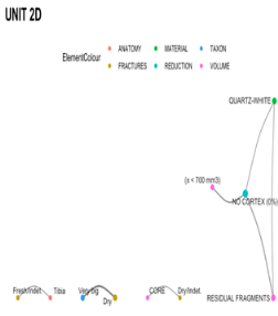
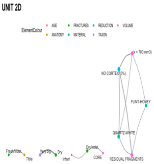
Heritage 07 00211 i001Heritage 07 00211 i002
UNIT 3E (603 artefacts)Threshold 46%Threshold 40%
1. A looped link between non-cortex stones, grey flint, and small flakes (30 mm3 < x < 700 mm3).
2. A relationship between white quartz and small flakes (30 mm3 < x < 700 mm3).
3. A correlation between adult faunal rests and non-cortex stones.
4. An association between lithic industry (1200 mm3 < x < 5000 mm3) and non-cortex traits.
5. A connection of grey diorite with residual fragments (debris) and all-cortex stones.
6. A tie between honey-coloured Otero flint, residual fragments (debris), and medium-sized lithic industry (700 mm3 < x < 1200 mm3).
7. A presence of core lithic pieces associated with some cortex (75–50%).
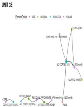
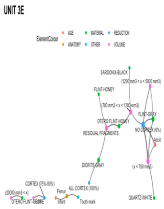
Heritage 07 00211 i003Heritage 07 00211 i004
UNIT 3F (506 artefacts)Threshold 46%Threshold 40%
1. An association among black-coloured thermo-alterations and adult faunal remains.
2. A relationship between big/medium-sized animals and humerus remnants.
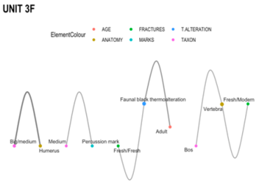
Heritage 07 00211 i005Heritage 07 00211 i006
UNIT 3G (993 artefacts)Threshold 46%Threshold 40%
1. An association among black-coloured thermo-alterations and adult faunal remains.
2. A correlation between grey flint and a flat butt, pronounced bulb, and unipolar dorsal (FPU) flaking.
3. A connection between cut marks, the Equus genus rests, and fresh/indeterminate fractures.
4. A linkage between big-sized faunal rests with percussion marks.
Heritage 07 00211 i007Heritage 07 00211 i008
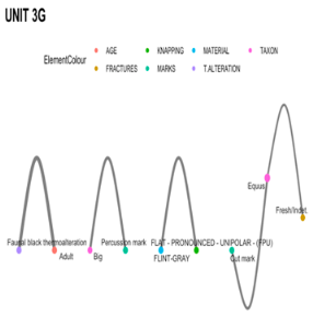
UNIT 4H (32 artefacts)
The tibia and humerus bones are present in small quantities. There is a moderate amount of brown Otero flint, honey-coloured Otero flint, and stones with much cortex (99–75%). There is an accumulation of residual fragments and a medium-sized lithic industry (1200 mm3 < x < 5000 mm3). There are no patent correlations between the components mentioned above.
UNIT 4I (1 artefact)
Sterile.
UNIT 4J (5 artefacts)
Sterile.
UNIT 5K (1531 artefacts)Threshold 46%Threshold 40%
1. A robust correlation among vertebra, sesamoid, and phalanx bones in connection with senile carnivore rests (Canis lupus) and fresh/modern, indeterminate/indeterminate fractures.
2. A solid association between a flat butt, little pronounced bulb, and indeterminate dorsal (FLPI) flaking connected with non-cortex brown Otero flint, brown jasper, and white quartz with volumes that vary from 30 mm3 to 20,000 mm3.
3. A firm tie between some-cortex (75–50%) stones connected with (1200 mm3 < x < 20,000 mm3)-sized lithic industry.
4. A steady relationship between small flakes (30 mm3 < x < 700 mm3) and a flat butt, pronounced bulb, and indeterminate dorsal (FPI) flaking.
5. A robust correlation between a flat butt, non-pronounced bulb, and indeterminate dorsal (FNPI) flaking with (1200 mm3 < x < 5000 mm3) lithic size.
Heritage 07 00211 i009Heritage 07 00211 i010
Total: 4190 artefacts in the excavation134 connections achieved (0.3%)205 connections achieved (0.47%)
Table 10. Network analysis statistics for 46% threshold.
Lithostratigraphic UnitDegree of CentralityCentral NodeBetweenness CentralityCloseness
2D38 No cortex (0%),
24 Residual fragment.
No cortex (0%).No cortex.
  • Tibia/fresh-indet./dry/very big/core.
3E62 No cortex (0%),
44 30 mm3 < x < 700 mm3.
No cortex (0%).No cortex.
  • Core/cortex (75–50%).
3F12 Humerus,
12 Big/medium-sized.
Humerus/big-medium-sized.-
  • Humerus/big-medium/adult/faunal black alt.
3G44 Equus sp.,
26 Adult.
Equus sp.Equus sp.
  • Percussion marks/big/adult/faunal black alt./FPU/grey flint.
5K324 Senile,
320 Carnivore.
Senile.1200 mm3 < x < 5000 mm3.
  • Carnivore/senile.
Table 11. Network analysis statistics for 40% threshold.
Lithostratigraphic UnitDegree of CentralityCentral NodeBetweenness CentralityCloseness
2D38 No cortex (0%),
32 Residual fragment.
No cortex (0%).Residual fragment.
  • Tibia/fresh-indet./dry/very big.
3E74 No cortex (0%),
56 30 mm3 < x < 700 mm3.
No cortex (0%).30 mm3 < x < 700 mm3.
  • Grey Otero flint/core/cortex(75–50%)/x > 20,000 mm3.
3F18 Faunal black alter.,
16 Vertebra.
Faunal black alter.Faunal black alter.
  • Humerus/big-medium/percussion marks.
3G82 Adult,
82 FPU.
Adult/FPU.Big/medium-sized.
  • Rib/small/fox/grey diorite/pseudo-retouched.
5K380 Senile,
376 Carnivore.
Senile.Brown jasper.
  • Carnivore/senile.
Disclaimer/Publisher’s Note: The statements, opinions and data contained in all publications are solely those of the individual author(s) and contributor(s) and not of MDPI and/or the editor(s). MDPI and/or the editor(s) disclaim responsibility for any injury to people or property resulting from any ideas, methods, instructions or products referred to in the content.

