
Photometric Stereo Techniques for the 3D Reconstruction of Paintings and Drawings Through the Measurement of Custom-Built Repro Stands


Abstract
:1. Introduction
- Digital representations based on images with a very high density of spatial content (i.e., the so-called gigapixel images). This solution is well illustrated by the Rijksmuseum’s 2019 gigantic Operation Night Watch project, which was able to reproduce Rembrandt’s painting with a resolution of 5 µm using 717 billion pixels [3].
- Images from Dome Photography (DP) that can be used in three ways: (1) visualization of the surface behavior of the artwork through the interactive movement of a virtual light source over the enclosing hemisphere, i.e., the Reflectance Transformation Images (RTI) [4]; (2) a 3D reconstruction of the object surface; (3) the modeling of the specular highlights from the surface and hence a realistic rendering.
- The visualization of the artwork in a digital context that simulates the three-dimensional environment in which it is placed;
- The free exploration of the painting or drawing, allowing users to zoom in on details, to observe surface behaviors under changing lighting conditions and at different angles, and to manipulate the artifact in real-time ‘as in your hands’ [6];
- The reproduction of the shape and the optical properties of the materials that make up the artwork, i.e., their total appearance [7].
2. The Photometric Stereo Framework
2.1. State of the Art
2.2. The Adopted PS Solution
- Albedo map;
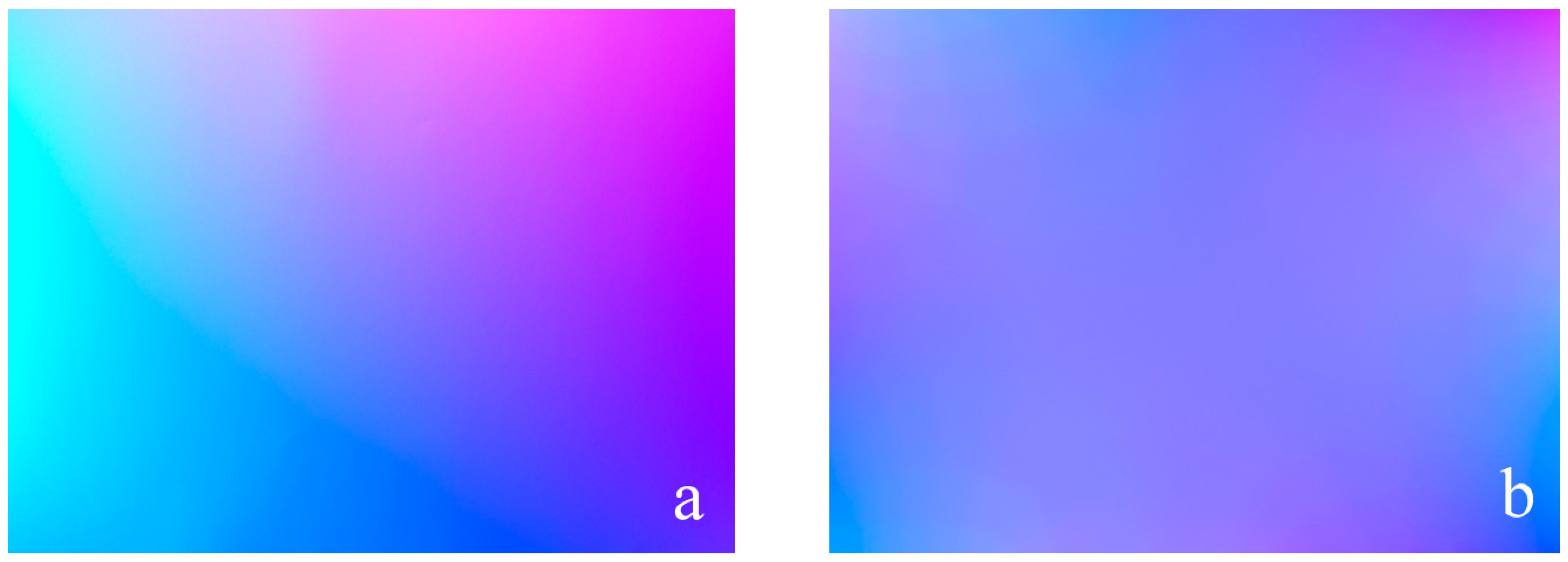
- Normal map;
- Depth map, by integration of estimated normal vector field;
- Reflection map generated as the difference in the apparent color with the albedo;
- Mesh with a resolution of a vertex for each pixel (i.e., 40 μm) exploiting the MATLAB functions surfaceMesh and meshgrid. In practice, for each pixel, a vertex is generated with coordinates x, y. The z depth is derived from the depth map, and finally a Delaunay triangulation generates the mesh. The mesh spatial density parameters can be adjusted through quadric decimation.
- Circle fitting from manually selected points on a chrome sphere image;
- Light direction determination using the chrome sphere image;
- Light strength estimation and lighting matrix refinement through nonlinear least squares optimization;
- PS computation to generate albedo and normal maps;
- Depth map reconstruction through the integration of the estimated normal vector field.
- Lack of precision at the border of rectangular domains, if the boundaries are not constrained;
- Inaccuracies for very low frequencies, although the photometric gradients provide a good representation of the spatial frequencies in the surface, right up to the Nyquist frequency. Errors can result in ‘curl’ or ‘heave’ in the base plane [59].
- A.
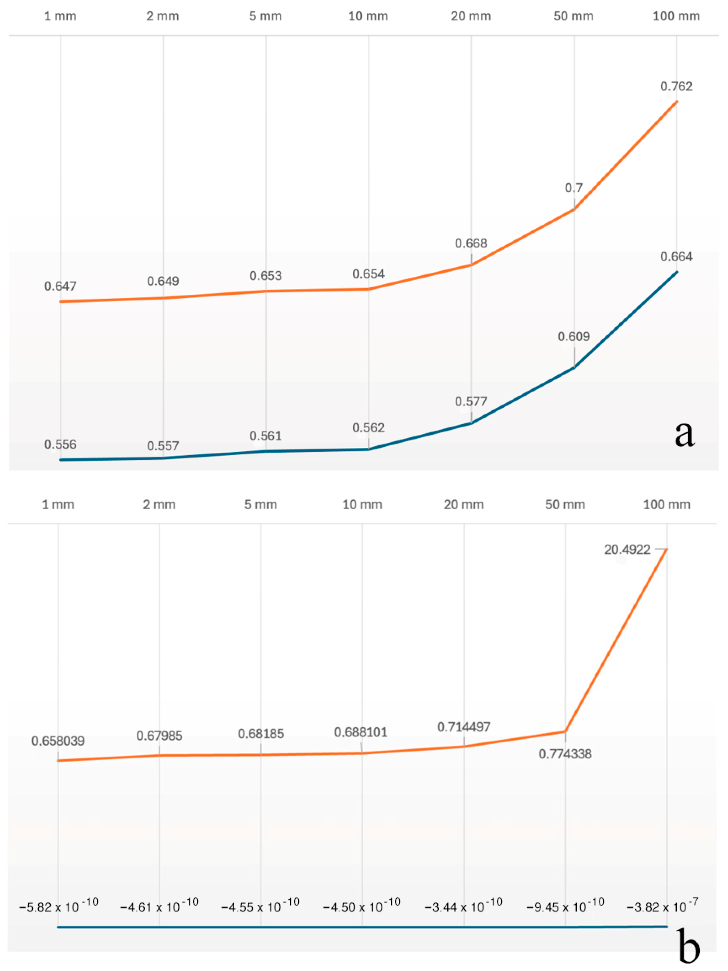
- A nearby light source model is used, so they can be modeled as a distant point light (this is possible when the working distance from an illuminator to an object surface is more than five times the maximum dimension of the light-emitting area) [60]. The position and direction of the light are found through measurement of the mutual position of the camera, lights, and acquisition plane. This geometric constraint provides a robust and deterministic approach, as the spatial relationships between points are predetermined by the physical setup rather than relying on potentially error-prone manual fitting operations. We evaluated the required accuracy of the measurement of the components’ mutual position through a series of tests aiming to evaluate the maximum possible error. At the end of the PS process, the maximum errors need to be as follows:
- No more than 0.1 pixels in the final normal map (maximum angular difference of 0.5° in the evaluation of the direction of the normal);
- No more than 1 mm in the mesh.
- B.
- Frankot and Chellappa’s method for normal integration failures is corrected following a series of observations. As noted in [22], the accuracy of Frankot and Chellappa’s method ‘relies on a good input scale’ and a big improvement could be achieved through exploiting solutions that are able to run on non-periodic surfaces (“The fact that the solution [of Frankot and Chellappa] is constrained to be periodic leads to a systematic bias in the solution” [61]) and to manage a non-rectangular domain. The latter condition is negligible in our case because paintings and drawings usually have a rectangular domain or—if not—can easily be inscribed into a rectangle anyway. We improved the other conditions, exploiting the solution suggested by Simchony et al. [62], which consists of solving the discrete approximation of the Poisson equation using discrete Fourier transform instead of discretizing the solution of the Poisson.
- C.
- The most common solution to the problem of the wrong representation of the surface at low frequencies is to replace the inaccurate low frequencies of the photometric normal with the more accurate low frequencies of a surface constructed from a few known heights measured with a laser scanner, or a probe, or a photogrammetric process [20,63]. We developed a different process, like that proposed by [21], which also allowed us to minimize problems caused by other factors, such as shadows, irregularity in the light sources and their position, different brightnesses for each light source, and a lack of perfect parallelism among the light beams. We use the distribution of light irradiance sampled from a flat reference surface. The non-uniformity of the radiance distribution is compensated using the reference images. In practice, a flat surface is measured that covers the whole light field and the normal field is calculated. Different normal values are qualified as systematic distortions and their value is subtracted from the normal field of the represented object. With this solution, there is no additional significant time cost required to solve the PS problem, as the procedure remains a linear problem. Finally, a surface deformation correction is applied by a 3 × 3 three-dimensional parabolic fitting algorithm, exploiting the MATLAB function fit and minimizing the error at the least squares at all the points of the surface [64].
2.3. The Hardware Solutions
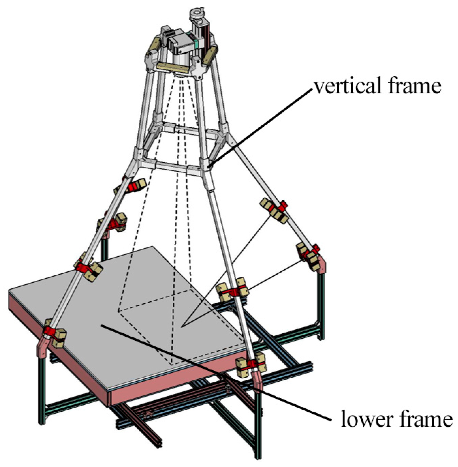
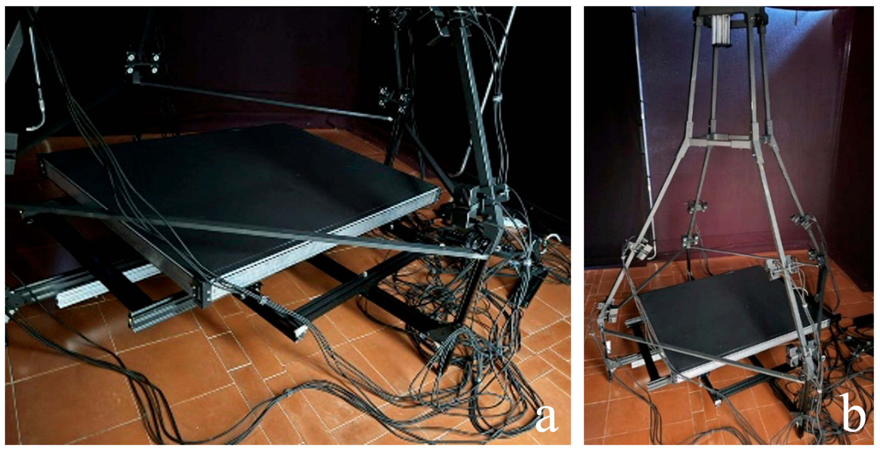
2.3.1. The Horizontal Stand
- A lower frame with a capture surface (Figure 5a), consisting of a sliding base equipped with rails for translation along both the axes of the acquisition plane. This frame weighs 14 kg;
- A vertical frame system (Figure 5b), designed to house 32 Relio2 LED lights and camera, composed of four uprights made from square aluminum profiles, held in place by components manufactured through 3D rapid prototyping. This frame weighs 6 kg.
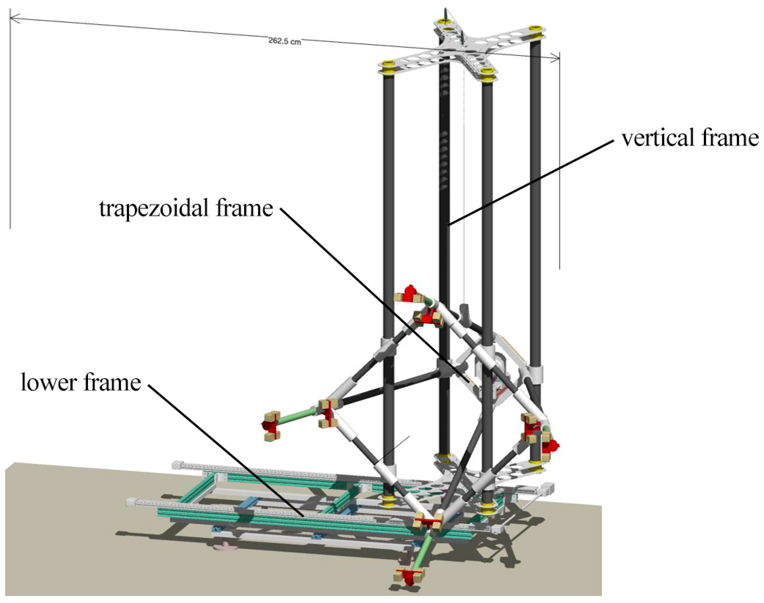
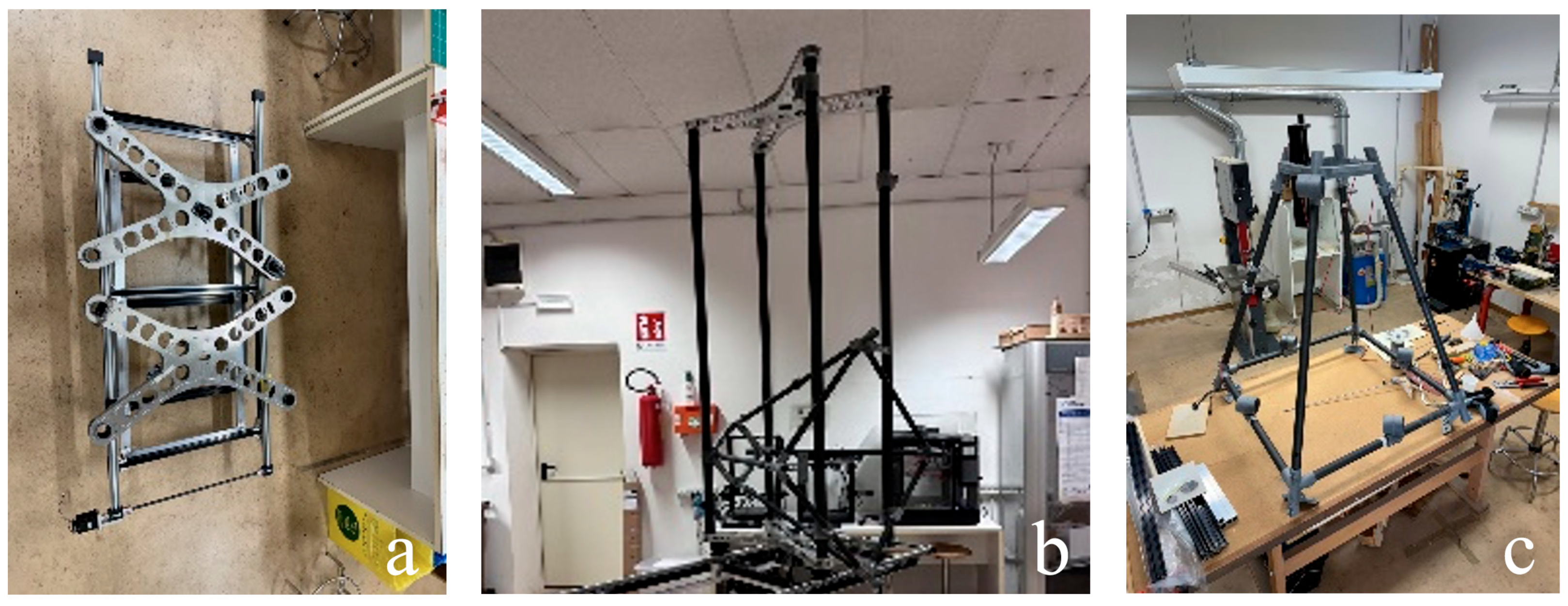
2.3.2. The Vertical Stand
- A lower frame (1800 × 1100 × 400 mm), consisting of a raisable base equipped with a rail for translation along the horizontal axis of the entire structure. The raisable base comprises a lifting frame that can be disassembled into individual arms (300 or 600 mm long) (Figure 7a). This frame weighs 35 kg (including the lifting frame and its ballasts);
- A vertical frame system composed of four carbon fiber uprights held in place by two lightweight aluminum cross-braces (Figure 7b). This frame weighs 3 kg;
- A trapezoidal frame (850 × 850 × 1200 mm) to which 32 Relio2 LED lights and the mounting system for the camera are secured (Figure 7c). This frame weighs 10 kg. The capture area is 500 × 375 mm on the acquisition plane, per single shot.
3. The Measurement Methodology
3.1. Metrological Context and Approach
3.2. The Instruments Used for Measurements
3.2.1. Scantech iReal M3 Laser Scanner
3.2.2. Laser Scanner Leica RTC360 Tof TLS System
3.2.3. Hasselblad X2D-100C Camera
3.3. Calibration and Characterization of Measurement Instruments
3.3.1. Calibration and Characterization of the Scantech iReal M3 Laser Scanner
3.3.2. Characterization of the Leica RTC360 ToF TLS System
3.3.3. Camera Calibration
- Focal length (f): expressed in pixels.
- Principal point coordinates (Cx, Cy): defined as the coordinates of the intersection point of the optical axis with the sensor plane, expressed in pixels.
- Affinity and non-orthogonality coefficients (b1, b2): expressed in pixels.
- Radial distortion coefficients (k1, k2, k3): dimensionless.
- Tangential distortion coefficients (p1, p2): dimensionless.
3.4. Description of the Measurement Processes
- The acquisition of a series of coded RAD targets using the Scantech iReal M3 3D laser scanner to provide a metric reference to scale the model in the photogrammetric process (Section 3.4.1);
- The acquisition of the stands by the Leica RTC360 ToF TLS system (Section 3.4.2);
- The acquisition of the stands by photogrammetry (Section 3.4.3);
- The comparison of the photogrammetric data with the Leica RTC360 ToF TLS system data (Section 3.4.4).
3.4.1. Target Acquisition Through Scantech iReal M3 3D Laser Scanner
3.4.2. Stand Acquisition with Leica RTC360 ToF TLS System
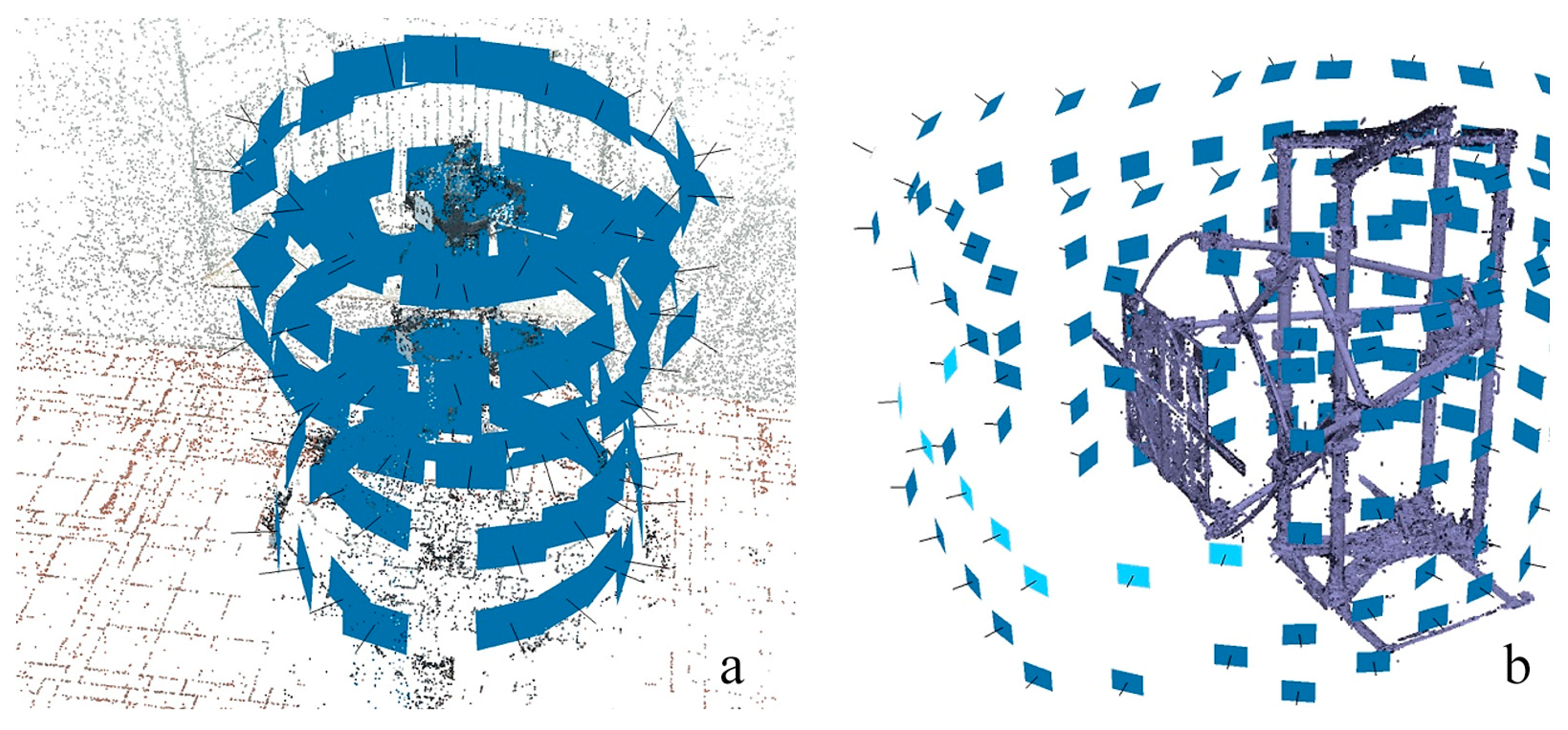
3.4.3. Stand Acquisition with Photogrammetry
- D is the distance in mm from the acquisition plane;
- Sw is the camera sensor width expressed in mm (equal to 43.8 mm for the Hasselblad X2D-100C);
- imW is the image width expressed in pixels (equal to 11,656 pixels for the Hasselblad X2D-100C output);
- Fr is the focal length of the adopted lens expressed in mm (equal to 38 mm for the Hasselblad XCD 38 mm f/2.5 V lens).
- n. 132 for the horizontal acquisition stand;
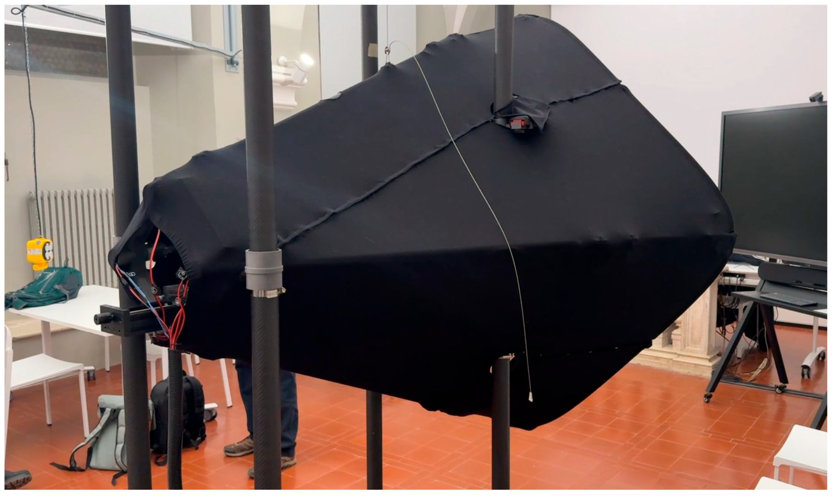
- n. 133 for the vertical robotic stand without darkening occlusion;
- n. 102 for the vertical robotic stand with darkening occlusion.
- Run the alignment procedure on the full set of captured images;
- Check the reprojection error on the resulting tie points. If below 0.5 pixels, stop here; otherwise, proceed with the next step;
- Delete about the 10% of the tie points providing the higher reprojection error;
- Rerun the BA step on the cleaned set of tie points and go back to step 2.
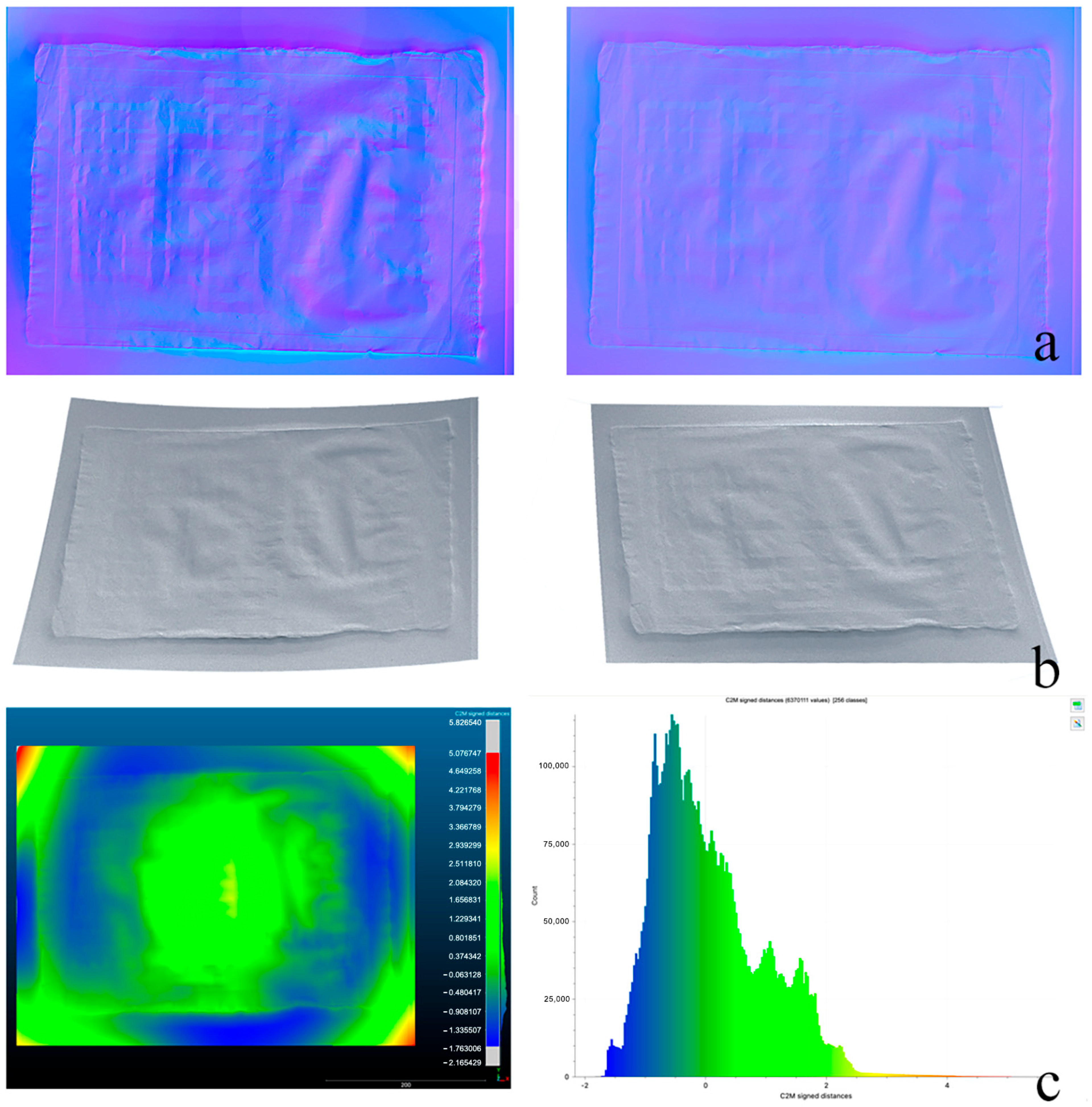
3.4.4. Comparison of the Photogrammetric and TLS Data
4. Results
4.1. As-Built Measurement of the Horizontal Repro Stand
4.1.1. Measurement Using Scantech iReal M3 Laser Scanner
4.1.2. Measurement Using Leica RTC360 ToF TLS System
4.1.3. Measurement with Photogrammetry
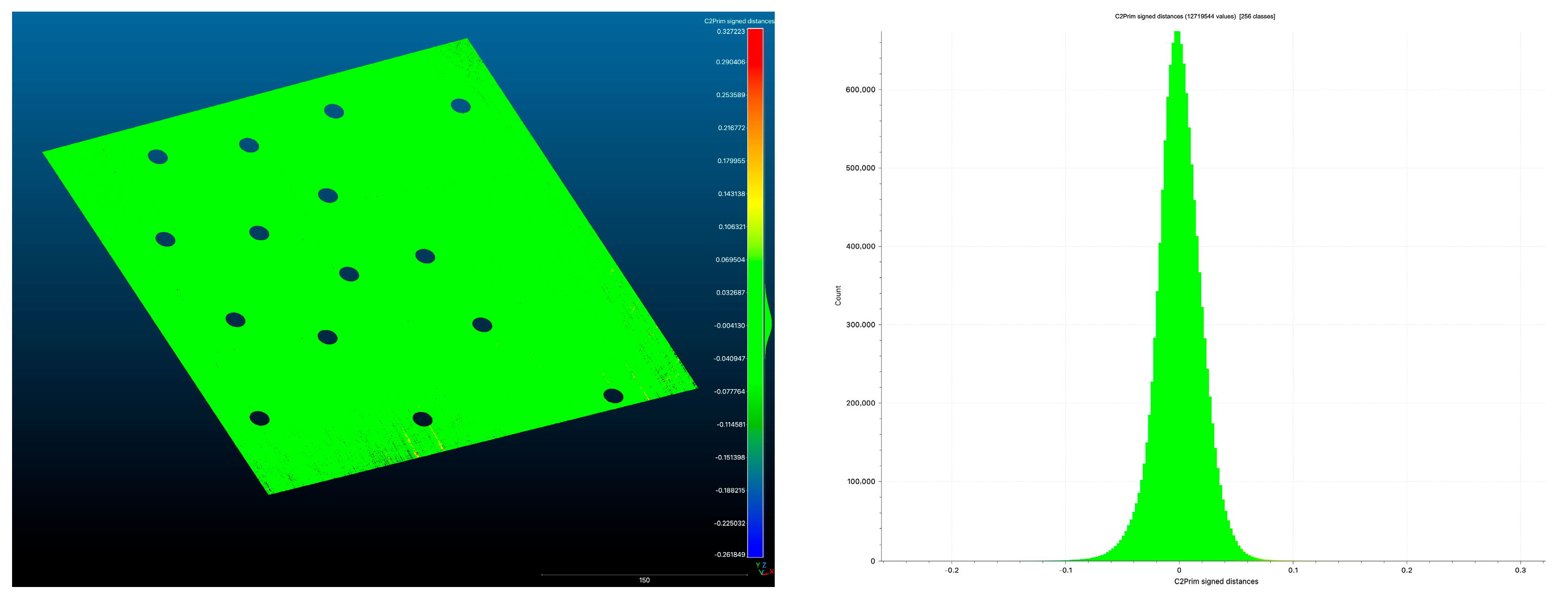
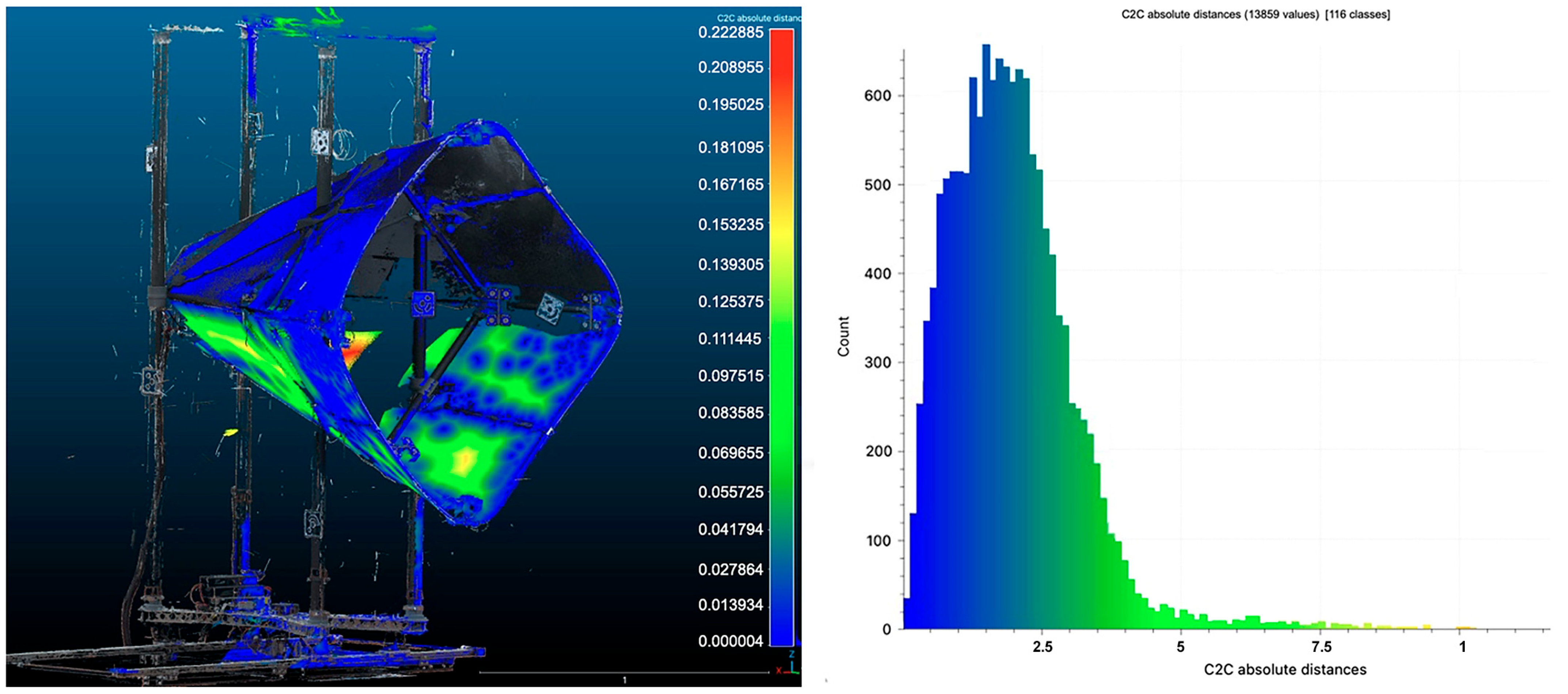
4.1.4. Comparison Between ToF TLS and Photogrammetry
4.1.5. Measurement of Points of Interest (PoIs) for the Horizontal Repro Stand
4.2. As-Built Measurement of the Robotic Vertical Repro Stand
4.2.1. Measurement Using Scantech iReal M3 Laser Scanner
4.2.2. Measurement Using Leica RTC360 ToF TLS System
4.2.3. Measurement with Photogrammetry
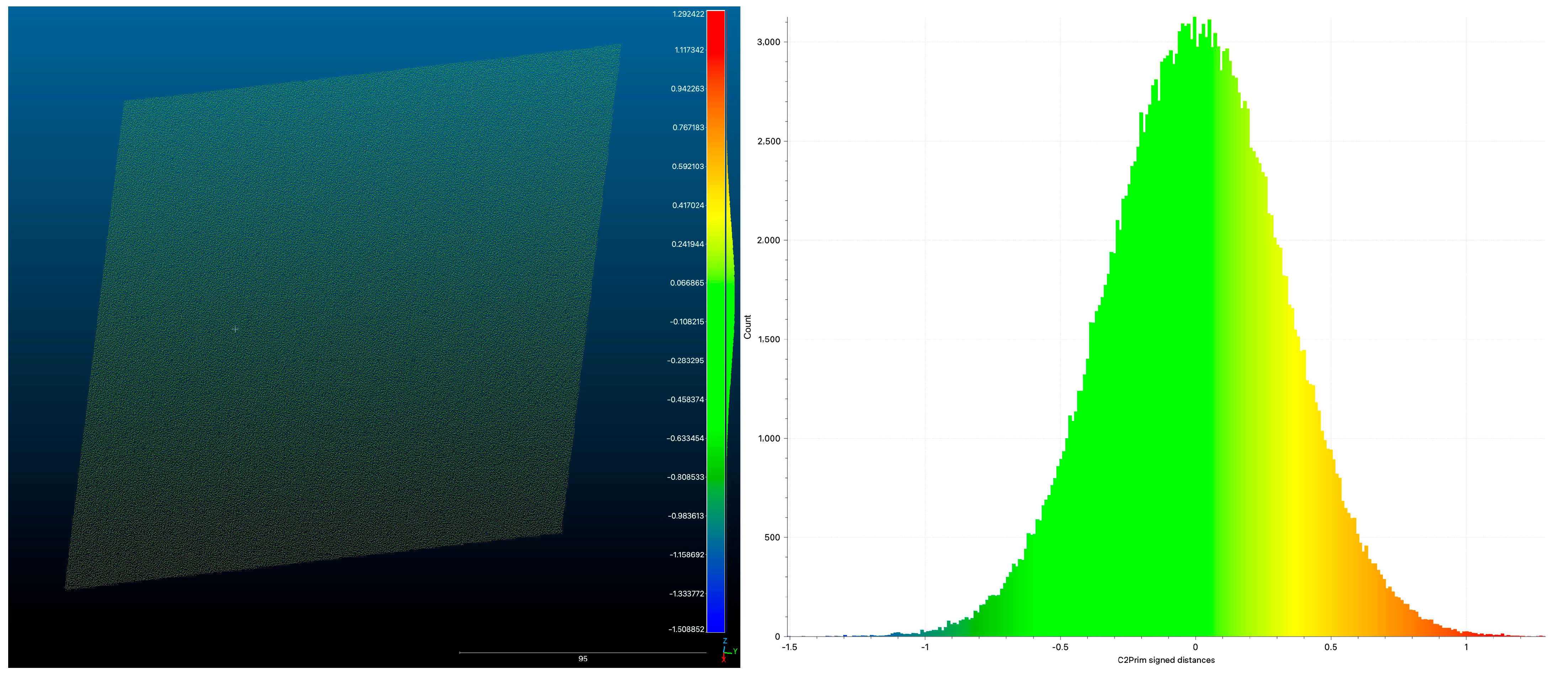
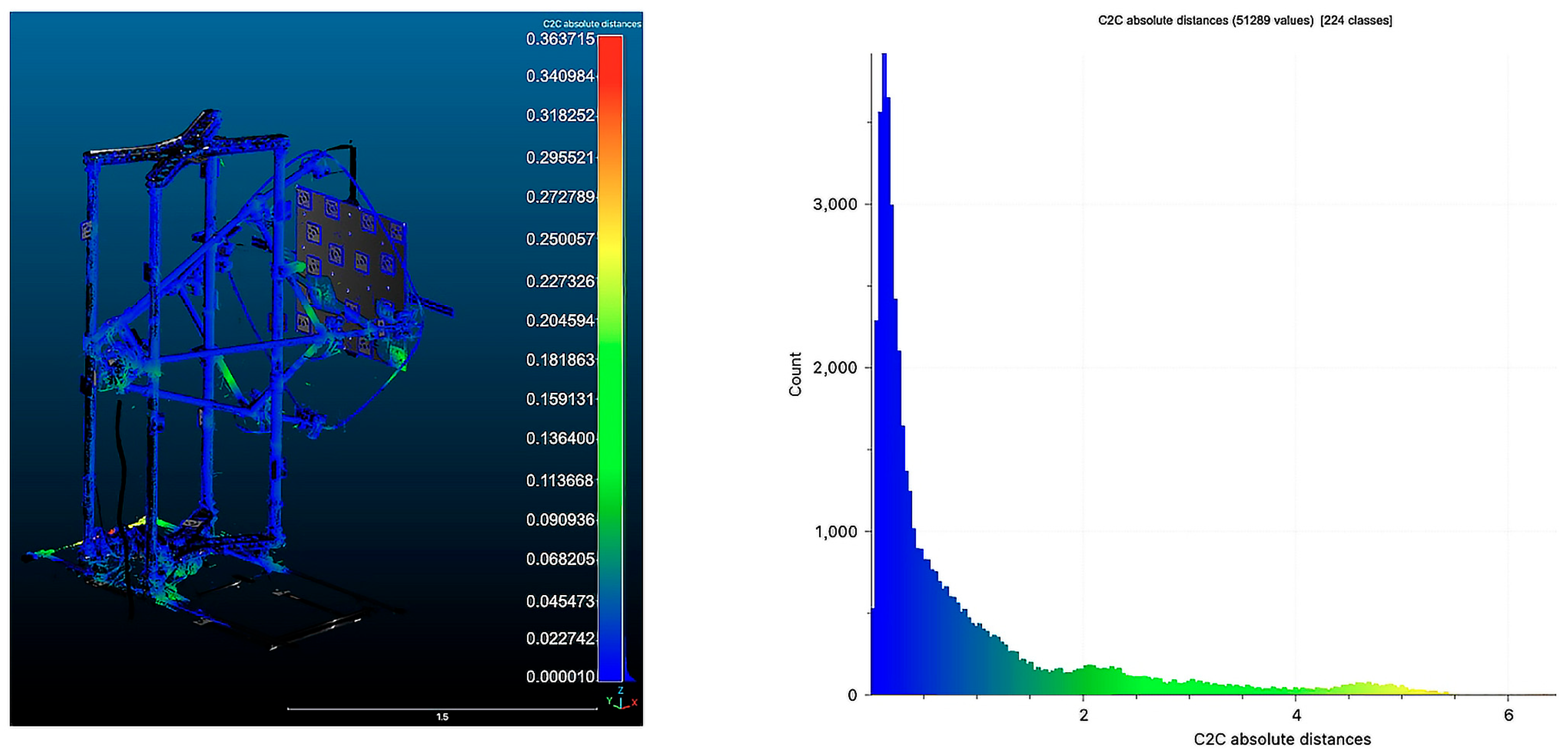
4.2.4. Comparison Between ToF TLS and Photogrammetry
4.2.5. Measurement of Points of Interest (PoIs) for the Vertical Repro Stand
4.3. Results Following the Performance Optimization of the PS Techniques
5. Discussion
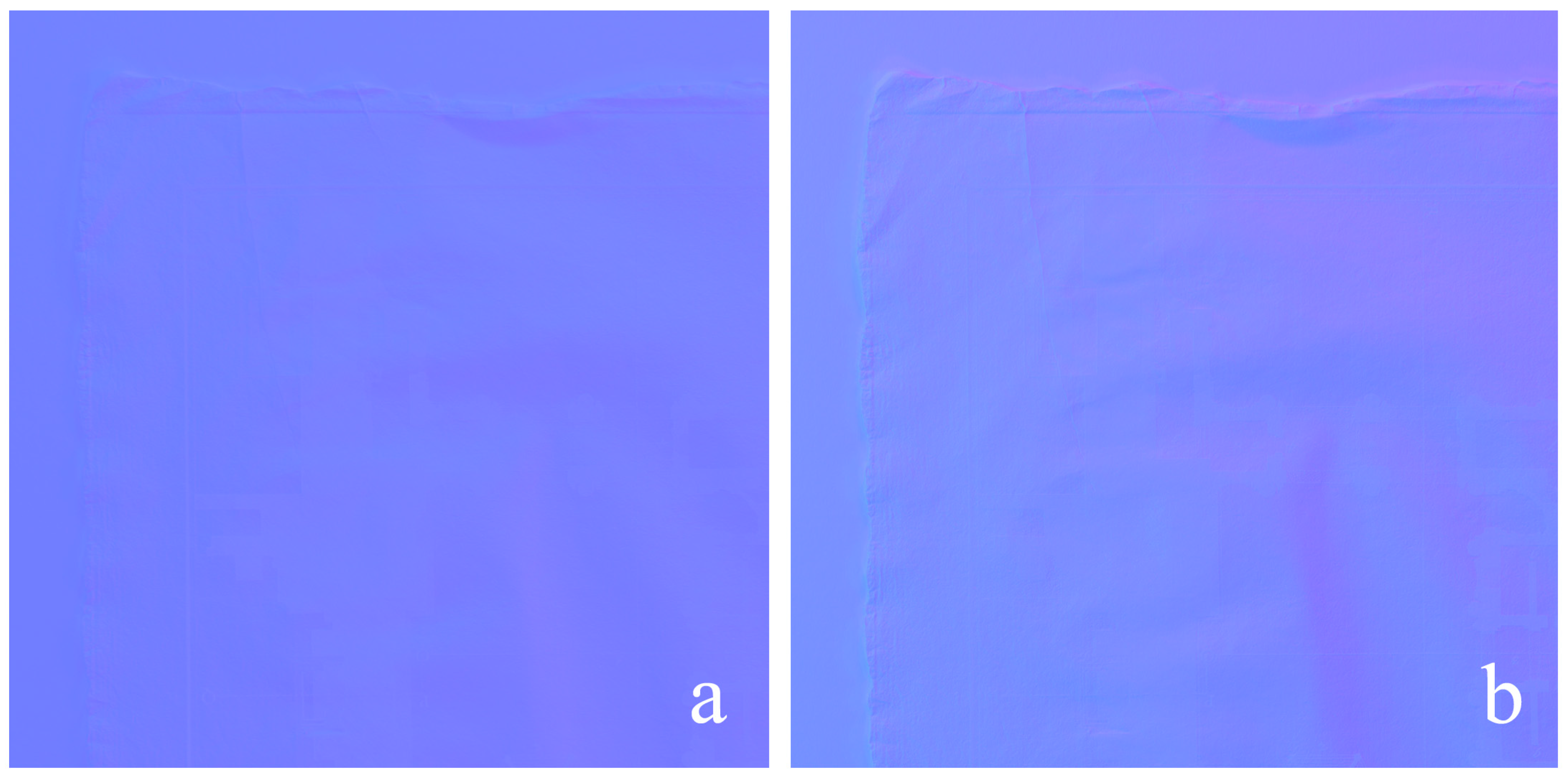
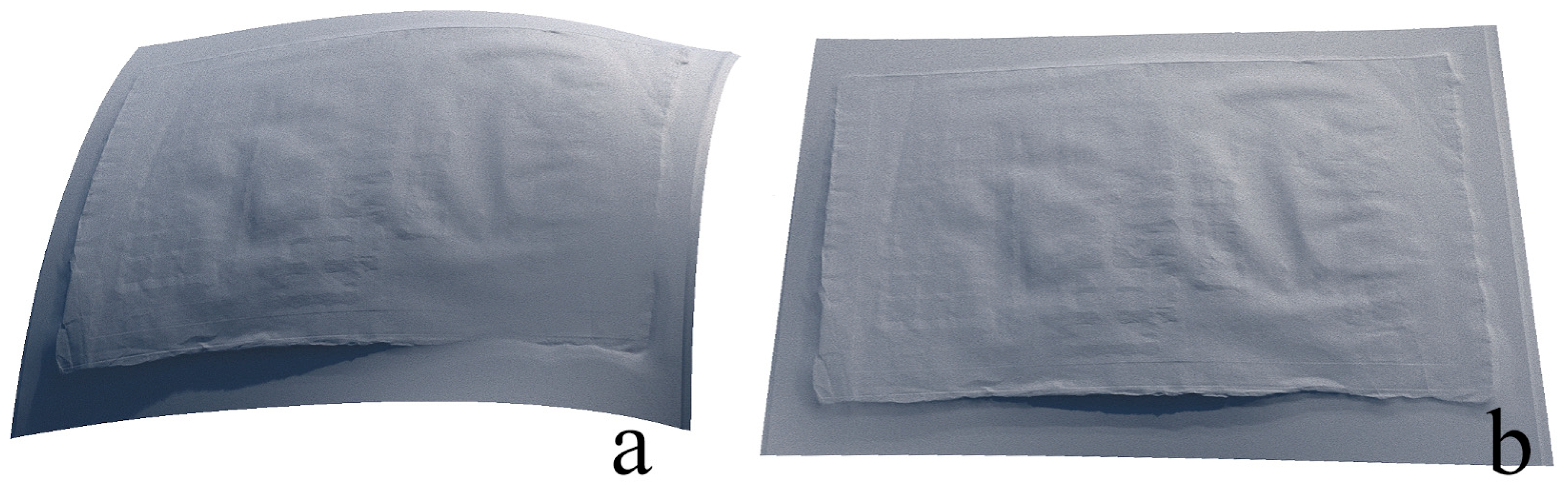
- An incorrect normal estimation often leads to warped surface reconstructions: one of our goals was to minimize distortions in the production of 3D meshes inferred from normal map integration. This proved to be achievable through the rigorous measurement of positions for lights, camera, and the acquisition plane. In the Section 4, we demonstrated that distortions in specific of paintings and drawings obtained using our measured solutions are mostly negligible.
- The accuracy of PS is heavily dependent on precise light positioning. Any misalignment in light direction or intensity estimation introduces errors in the 3D model: for this reason, we decided to measure the stands and elements’ positions to obtain an accurate layout that can be used more than once with the same level of accuracy.
- PS assumes surfaces reflect light evenly (Lambertian), but paintings and drawings have specular highlights, shadows, and non-uniform textures, and this affects normal estimation, leading to inaccuracies. We minimized the error in normal estimation using the following two strategies: 1. the non-Lambertian effect manifests more prominently at the edges of the shots, but we do not consider these due to the stitching, especially in wide paintings, which introduces a strong overlap between the captures; 2. the calibration process on a plane tends to minimize the effects of non-Lambertian surfaces. Certainly, in cases with extremely glossy surfaces, the problem remains, but it can be eliminated through the use of polarization techniques, which remain a future possibility for our solution.
- The horizontal and vertical repro stands are designed for medium-sized paintings and drawings. Larger artworks require stitching multiple images, which can introduce misalignment errors: our stands can deal with larger artworks, especially the vertical one, which has a robotized movement and can be shifted and/or lifted. The system is carefully leveled using a spherical level, with laser distance meters that ensure parallelism with the acquisition plane during the translation of the stand. In this way, misalignment errors are already minimized at the time of shooting.
- While stable, the repro lacks full automation, requiring manual adjustments. Vibrations, misalignment, or uneven placement of the artwork can introduce minor distortions: our stands, particularly the robotized vertical one, are equipped with vibration sensors that can check and avoid possible blurring in the captured images.
- The PSBox software that was initially used has limitations in accurately estimating surface normals. Frankot and Chellappa’s normal integration method fails to estimate object edges, causing inaccuracies in the reconstruction of detailed textures: we considered these criticalities, but we did not detail them as they are already well described in the literature [22]. In our solution, we adopted the natural boundary condition formulated by Neumann to overcome this issue, but details on its implementation are beyond the innovations presented in this paper.
6. Conclusions
- The integration of Deep Learning-based PS methods for better shadow handling and normal estimation;
- The use of AI-driven light calibration to dynamically adjust illumination parameters;
- The implementation of multi-spectral imaging to better differentiate material properties;
- Hybrid reconstruction using Machine Learning to improve shape recovery, even for highly textured or reflective surfaces;
- The addition of fully automated scanning systems with AI-based positioning and lighting control and the care to copyrights from a digital perspective [108];
Author Contributions
Funding
Data Availability Statement
Acknowledgments
Conflicts of Interest
References
- Apollonio, F.I.; Bacci, G.; Ballabeni, A.; Foschi, R.; Gaiani, M.; Garagnani, S. InSight Leonardo—ISLE. In Leonardo, Anatomia dei Disegni; Marani, P., Ed.; Sistema Museale di Ateneo Università di Bologna: Bologna, Italy, 2019; pp. 31–45. [Google Scholar]
- Gaiani, M.; Garagnani, S.; Zannoni, M. Artworks at our fingertips: A solution starting from the digital replication experience of the Annunciation in San Giovanni Valdarno. Digit. Appl. Archaeol. Cult. Herit. 2024, 33, e00329. [Google Scholar]
- Operation Night Watch at Rijks Museum. Available online: https://www.rijksmuseum.nl/en/stories/operation-night-watch/story/ultra-high-resolution-photo (accessed on 9 January 2025).
- Malzbender, T.; Gelb, D.; Wolters, H. Polynomial Texture Maps. In Proceeding of the 28th Annual Conference on Computer Graphics and Interactive Techniques (SIGGRAPH ‘01); ACM: New York, NY, USA, 2001; pp. 519–528. [Google Scholar]
- Gaiani, M.; Apollonio, F.I.; Ballabeni, A.; Bacci, G.; Bozzola, M.; Foschi, R.; Garagnani, S.; Palermo, R. Vedere Dentro i Disegni. Un Sistema per Analizzare, Conservare, Comprendere, Comunicare i Disegni di Leonardo. In Leonardo a Vinci, Alle Origini del Genio; Barsanti, R., Ed.; Giunti Editore: Milano, Italy, 2019; pp. 207–240. [Google Scholar]
- Apollonio, F.I.; Gaiani, M.; Garagnani, S.; Martini, M.; Strehlke, C.B. Measurement and restitution of the Annunciation by Fra Angelico in San Giovanni Valdarno. Disegnare Idee Immagin. 2023, 34, 32–47. [Google Scholar]
- Eugène, C. Measurement of “total visual appearance”: A CIE challenge of soft metrology. In Proceedings of the 12th IMEKO TC1 & TC7 Joint Symposium on Man, Science & Measurement Proceedings, Annecy, France, 3–5 September 2008; pp. 61–65. Available online: https://www.imeko.org/publications/tc7-2008/IMEKO-TC1-TC7-2008-006.pdf (accessed on 9 January 2025).
- Anderson, B.L. Visual perception of materials and surfaces. Curr. Biol. 2011, 21, 978–983. [Google Scholar]
- Woodham, R.J. Photometric method for determining surface orientation from multiple images. Opt. Eng. 1980, 19, 139–144. [Google Scholar] [CrossRef]
- Cook, R.L.; Torrance, K.E. A reflectance model for computer graphics. ACM Trans. Graph. 1982, 1, 7–24. [Google Scholar]
- Sole, A.; Farup, I.; Nussbaum, P.; Tominaga, S. Bidirectional reflectance measurement and reflection model fitting of complex materials using an image-based measurement setup. J. Imaging 2018, 4, 136. [Google Scholar] [CrossRef]
- Gaiani, M.; Ballabeni, A. SHAFT (SAT & HUE Adaptive Fine Tuning), a New Automated Solution for Target-Based Color Correction. In Colour and Colorimetry Multidisciplinay Contributions; Marchiafava, V., Luzzatto, L., Eds.; Gruppo del Colore—Associazione Italiana Colore: Milan, Italy, 2018; Volume XIV B, pp. 69–80. [Google Scholar]
- Gaiani, M.; Apollonio, F.I.; Clini, P. Innovative approach to the digital documentation and rendering of the total appearance of fine drawings and its validation on Leonardo’s Vitruvian Man. J. Cult. Herit. 2015, 16, 805–812. [Google Scholar]
- Apollonio, F.I.; Foschi, R.; Gaiani, M.; Garagnani, S. How to Analyze, Preserve, and Communicate Leonardo’s Drawing? A Solution to Visualize in RTR Fine Art Graphics Established from “the Best Sense”. ACM J. Comput. Cult. Herit. 2021, 14, 36. [Google Scholar] [CrossRef]
- MacDonald, L.W.; Nocerino, E.; Robson, S.; Hess, M. 3D Reconstruction in an Illumination Dome. In Proceedings of the Electronic Visualisation and the Arts (EVA), London, UK, 9–13 July 2018; pp. 18–25. [Google Scholar]
- Apollonio, F.I.; Gaiani, M.; Garagnani, S. Visualization and Fruition of Cultural Heritage in the Knowledge-Intensive Society: New Paradigms of Interaction with Digital Replicas of Museum Objects, Drawings, and Manuscripts. In Handbook of Research on Implementing Digital Reality and Interactive Technologies to Achieve Society 5.0; Ugliotti, F.M., Osello, A., Eds.; IGI Global: Hershey, PA, USA, 2022; pp. 471–495. [Google Scholar]
- Karami, A.; Menna, F.; Remondino, F. Combining Photogrammetry and Photometric Stereo to Achieve Precise and Complete 3D Reconstruction. Sensors 2022, 22, 8172. [Google Scholar] [CrossRef]
- Bacci, G.; Bozzola, M.; Gaiani, M.; Garagnani, S. Novel Paradigms in the Cultural Heritage Digitization with Self and Custom-Built Equipment. Heritage 2023, 6, 6422–6450. [Google Scholar] [CrossRef]
- Huang, X.; Walton, M.; Bearman, G.; Cossairt, O. Near light correction for image relighting and 3D shape recovery. In Proceedings of the Digital Heritage, Granada, Spain, 28 September–2 October 2015; pp. 215–222. [Google Scholar]
- Macdonald, L.W. Representation of Cultural Objects by Image Sets with Directional Illumination. In Proceedings of the 5th Computational Color Imaging Workshop—CCIW, Saint Etienne, France, 24–26 March 2015; pp. 43–56. [Google Scholar]
- Sun, J.; Smith, M.; Smith, L.; Farooq, A. Sampling Light Field for Photometric Stereo. Int. J. Comput. Theory Eng. 2013, 5, 14–18. [Google Scholar] [CrossRef]
- Quéau, Y.; Durou, J.D.; Aujol, J.F. Normal Integration: A Survey. J. Math. Imaging Vis. 2018, 60, 576–593. [Google Scholar] [CrossRef]
- Horovitz, I.; Kiryati, N. Depth from gradient fields and control points: Bias correction in photometric stereo. Image Vis. Comput. 2004, 22, 681–694. [Google Scholar] [CrossRef]
- MacDonald, L.W.; Robson, S. Polynomial texture mapping and 3D representation. In Proceedings of the ISPRS Commission V Symposium Close Range Image Measurement Techniques, Newcastle, UK, 21–24 June 2010. [Google Scholar]
- Antensteiner, D.; Štolc, S.; Pock, T. A review of depth and normal fusion algorithms. Sensors 2018, 18, 431. [Google Scholar] [CrossRef]
- Li, M.; Zhou, Z.; Wu, Z.; Shi, B.; Diao, C.; Tan, P. Multi-View Photometric Stereo: A Robust Solution and Benchmark Dataset for Spatially Varying Isotropic Materials. IEEE Trans. Image Process. 2020, 29, 4159–4173. [Google Scholar] [CrossRef] [PubMed]
- Rostami, M.; Michailovich, O.; Wang, Z. Gradient-based surface reconstruction using compressed sensing. In Proceedings of the 2012 19th IEEE International Conference on Image Processing (ICIP), Orlando, FL, USA, 30 September–3 October 2012; pp. 913–916. [Google Scholar]
- Solomon, F.; Ikeuchi, K. Extracting the shape and roughness of specular lobe objects using four light photometric stereo. IEEE Trans. Pattern Anal. Mach. Intell. 1996, 18, 449–454. [Google Scholar] [CrossRef]
- Barsky, S.; Petrou, M. The 4-source photometric stereo technique for three-dimensional surfaces in the presence of high-lights and shadows. IEEE Trans. Pattern Anal. Mach. Intell. 2003, 25, 1239–1252. [Google Scholar] [CrossRef]
- Cox, B.; Berns, R. Imaging artwork in a studio environment for computer graphics rendering. In Proceedings of the SPIE-IS&T Measuring, Modeling, and Reproducing Material Appearance, San Francisco, CA, USA, 9–10 February 2015. [Google Scholar]
- Ackermann, J.; Goesele, M. A survey of photometric stereo techniques. Found. Trends Comput. Graph. Vis. 2015, 9, 149–254. [Google Scholar]
- Belhumeur, P.N.; Kriegman, D.J.; Yuille, A.L. The Bas-Relief Ambiguity. Int. J. Comput. Vis. 1999, 35, 33–44. [Google Scholar] [CrossRef]
- Papadhimitri, T.; Favaro, P. A new perspective on uncalibrated photometric stereo. In Proceedings of the IEEE Computer Society Conference on Computer Vision and Pattern Recognition, Portland, OR, USA, 23–28 June 2013; pp. 1474–1481. [Google Scholar]
- Hertzmann, A.; Seitz, S. Shape and materials by example: A photo- metric stereo approach. In Proceedings of the IEEE Computer Society Conference on Computer Vision and Pattern Recognition, Madison, WI, USA, 18–20 June 2003. [Google Scholar]
- Alldrin, N.; Zickler, T.; Kriegman, D. Photometric stereo with non- parametric and spatially-varying reflectance. In Proceedings of the 26th IEEE Conference on Computer Vision and Pattern Recognition, Anchorage, AK, USA, 23–28 June 2008; pp. 1–8. [Google Scholar]
- Goldman, D.B.; Curless, B.; Hertzmann, A.; Seitz, S.M. Shape and spatially-varying BRDFs from photometric stereo. IEEE Trans. Pattern Anal. Mach. Intell. 2010, 32, 1060–1071. [Google Scholar] [CrossRef]
- Ren, J.; Jian, Z.; Wang, X.; Mingjun, R.; Zhu, L.; Jiang, X. Complex surface reconstruction based on fusion of surface normals and sparse depth measurement. IEEE Trans. Instrum. Meas. 2021, 70, 2506413. [Google Scholar] [CrossRef]
- Wu, L.; Ganesh, A.; Shi, B.; Matsushita, Y.; Wang, Y.; Ma, Y. Robust photometric stereo via low-rank matrix completion and recovery. In Proceedings of the 10th Asian Conference on Computer Vision, Computer Vision—ACCV, Queenstown, New Zealand, 8–12 November 2010; pp. 703–717. [Google Scholar]
- Ikehata, S.; Wipf, D.; Matsushita, Y.; Aizawa, K. Robust photometric stereo using sparse regression. In Proceedings of the IEEE Computer Society Conference on Computer Vision and Pattern Recognition, Providence, RI, USA, 16–21 June 2012; pp. 318–325. [Google Scholar]
- MacDonald, L.W. Colour and directionality in surface reflectance. In Proceedings of the Artificial Intelligence and the Simulation of Behaviour (AISB), London, UK, 1–4 April 2014; pp. 223–229. [Google Scholar]
- Zhang, M.; Drew, M.S. Efficient robust image interpolation and surface properties using polynomial texture mapping. EURASIP J. Image Video Process. 2014, 1, 25. [Google Scholar] [CrossRef]
- Sun, J.; Smith, M.; Smith, L.; Abdul, F. Examining the uncertainty of the recovered surface normal in three light photometric Stereo. J. Image Comput. Vis. 2007, 25, 1073–1079. [Google Scholar] [CrossRef]
- Shi, B.; Mo, Z.; Wu, Z.; Duan, D.; Yeung, S.; Tan, P. A Benchmark Dataset and Evaluation for Non-Lambertian and Uncalibrated Photometric Stereo. IEEE Trans. Pattern Anal. Mach. Intell. 2019, 41, 271–284. [Google Scholar] [CrossRef]
- Fan, H.; Qi, L.; Wang, N.; Dong, J.; Chen, Y.; Yu, H. Deviation correction method for close-range photometric stereo with nonuniform illumination. Opt. Eng. 2017, 56, 170–186. [Google Scholar] [CrossRef]
- Wetzler, A.; Kimmel, R.; Bruckstein, A.M.; Mecca, R. Close-Range Photometric Stereo with Point Light Sources. In Proceedings of the 2nd International Conference on 3D Vision, Tokyo, Japan, 8–11 December 2014; pp. 115–122. [Google Scholar]
- Papadhimitri, T.; Favaro, P.; Bern, U. Uncalibrated Near-Light Photometric Stereo. In Proceedings of the British Machine Vision Conference, Nottingham, UK, 1–5 September 2014; pp. 1–12. [Google Scholar]
- Quéau, Y.; Durou, J.D. Some Illumination Models for Industrial Applications of Photometric Stereo. In Proceedings of the SPIE 12th International Conference on Quality Control by Artificial Vision, Le Creusot, France, 3–5 June 2015. [Google Scholar]
- Mecca, R.; Wetzler, A.; Bruckstein, A.; Kimmel, R. Near field photometric stereo with point light sources. SIAM J. Imaging Sci. 2014, 7, 2732–2770. [Google Scholar] [CrossRef]
- Quéau, Y.; Durix, B.; Wu, T.; Cremers, D.; Lauze, F.; Durou, J.D. LED-based photometric stereo: Modeling, calibration and numerical solution. J. Math. Imaging Vis. 2018, 60, 313–340. [Google Scholar] [CrossRef]
- Zheng, Q.; Kumar, A.; Shi, B.; Pan, G. Numerical reflectance compensation for non-lambertian photometric stereo. IEEE Trans. Image Process. 2019, 28, 3177–3191. [Google Scholar] [CrossRef] [PubMed]
- Wang, X.; Jian, Z.; Ren, M. Non-lambertian photometric stereo network based on inverse reflectance model with collocated light. IEEE Trans. Image Process. 2020, 29, 6032–6042. [Google Scholar] [CrossRef]
- Wen, S.; Zheng, Y.; Lu, F. Polarization guided specular reflection separation. IEEE Trans. Image Process. 2021, 30, 7280–7291. [Google Scholar] [CrossRef]
- Nehab, D.; Rusinkiewicz, S.; Davis, J.; Ramamoorthi, R. Efficiently combining positions and normals for precise 3D geometry. ACM Trans. Graph. 2005, 24, 536–543. [Google Scholar]
- Vogiatzis, G.; Hernández, C.; Cipolla, R. Reconstruction in the round using photometric normals and silhouettes. In Proceedings of the IEEE Conference on Computer Vision and Pattern Recognition, New York, NY, USA, 17–22 June 2006; pp. 1847–1854. [Google Scholar]
- Peng, S.; Haefner, B.; Quéau, Y.; Cremers, D. Depth super-resolution meets uncalibrated photometric stereo. In Proceedings of the IEEE International Conference on Computer Vision Workshops, Venice, Italy, 22–29 October 2017; pp. 2961–2968. [Google Scholar]
- Durou, J.D.; Falcone, M.; Quéau, Y.; Tozza, S. A Comprehensive Introduction to Photometric 3D-reconstruction. In Advances in Photometric 3D-Reconstruction; Durou, J.D., Falcone, M., Quéau, Y., Tozza, S., Eds.; Springer Nature: Cham, Switzerland, 2010. [Google Scholar]
- PSBox—A Matlab Toolbox for Photometric Stereo. Available online: https://github.com/yxiong/PSBox (accessed on 9 January 2025).
- Frankot, R.T.; Chellappa, R. A method for enforcing integrability in shape from shading algorithms. IEEE Trans. Pattern Anal. Mach. Intell. 1988, 10, 439–451. [Google Scholar]
- MacDonald, L.W. Surface Reconstruction from Photometric Normals with Reference Height Measurements. Opt. Arts Archit. Archaeol. V 2015, 9527, 7–22. [Google Scholar]
- Ashdown, I. Near-Field photometry: Measuring and modeling complex 3-D light sources. In ACM SIGGRAPH 95 Course Notes—Realistic Input Realistic Images; ACM: New York, NY, USA, 1995; pp. 1–15. [Google Scholar]
- Harker, M.; O’Leary, P. Least squares surface reconstruction from measured gradient fields. In Proceedings of the IEEE Conference on Computer Vision and Pattern Recognition, Anchorage, AK, USA, 23–28 June 2008. [Google Scholar]
- Simchony, T.; Chellappa, R.; Shao, M. Direct analytical methods for solving Poisson equations in computer vision problems. IEEE Trans. Pattern Anal. Mach. Intell. 1990, 12, 435–446. [Google Scholar]
- Tominaga, R.; Ujike, H.; Horiuchi, T. Surface reconstruction of oil paintings for digital archiving. In Proceedings of the IEEE Southwest Symp. on Image Analysis and Interpretation, Austin, TX, USA, 23–25 May 2010; pp. 173–176. [Google Scholar]
- MATLAB Fitpoly33 Function. Available online: https://it.mathworks.com/help/curvefit/fit.html (accessed on 9 January 2025).
- Relio2. Available online: https://www.relio.it/ (accessed on 9 January 2025).
- Marrugo, A.G.; Gao, F.; Zhang, S. State-of-the-art active optical techniques for three-dimensional surface metrology: A review. J. Opt. Soc. Am. 2020, 37, B60–B77. [Google Scholar] [CrossRef]
- Beraldin, J.A.; Blais, F.; El-Hakim, S.F.; Cournoyer, L.; Picard, M. Traceable 3D Imaging Metrology: Evaluation of 3D Digitizing Techniques in a Dedicated Metrology Laboratory. In Proceedings of the 8th Conference on Optical 3D Measurement Techniques, Zurich, Switzerland, 9–12 July 2007; pp. 310–318. [Google Scholar]
- MacKinnon, D.; Aitken, V.; Blais, F. Review of measurement quality metrics for range imaging. J. Electron. Imaging 2008, 17, 033003-1–033003-14. [Google Scholar] [CrossRef]
- Givi, M.; Cournoyer, L.; Reain, G.; Eves, B.J. Performance evaluation of a portable 3D imaging system. Precis. Eng. 2019, 59, 156–165. [Google Scholar] [CrossRef]
- Beraldin, J.A.; Mackinnon, D.; Cournoyer, L. Metrological characterization of 3D imaging systems: Progress report on standards developments. In Proceedings of the 17th international congress of metrology, Paris, France, 21–24 September 2015. [Google Scholar]
- Beraldin, J.A. Basic theory on surface measurement uncertainty of 3D imaging systems. Three-Dimens. Imaging Metrol. 2009, 7239, 723902. [Google Scholar]
- Vagovský, J.; Buranský, I.; Görög, A. Evaluation of measuring capability of the optical 3D scanner. Procedia Eng. 2015, 100, 1198–1206. [Google Scholar] [CrossRef]
- Toschi, I.; Nocerino, E.; Hess, M.; Menna, F.; Sargeant, B.; MacDonald, L.W.; Remondino, F.; Robson, S. Improving automated 3D reconstruction methods via vision metrology. In Proceedings of the SPIE Optical Metrology, Munich, Germany, 22–23 June 2015. [Google Scholar]
- Guidi, G. Metrological characterization of 3D imaging devices. In Proceedings of the SPIE Optical Metrology, Munich, Germany, 14–15 May 2013. [Google Scholar]
- JCGM 200:2012; International Vocabulary of Metrology—Basic and General Concepts and Associated Terms (VIM), 3rd ed. BIPM: Sèvres, France, 2012.
- ISO 14253-2:2011; Guidance for the Estimation of Uncertainty in GPS Measurement, in Calibration of Measuring Equipment and in Product Verification. International Organization for Standardization: Geneva, Switzerland, 2011.
- Beraldin, J.A. Digital 3D Imaging and Modeling: A metrological approach. Time Compress. Technol. Mag. 2008, 33–35. [Google Scholar]
- MacKinnon, D.; Beraldin, J.A.; Cournoyer, L.; Blais, F. Evaluating Laser Spot Range Scanner Lateral Resolution in 3D Metrology. In Proceedings of the 21st Annual IS&T/SPIE Symposium on Electronic Imaging, San Jose, CA, USA, 18–22 January 2008. [Google Scholar]
- Nyquist, H. Thermal Agitation of Electric Charge in Conductors. Phys. Rev. 1928, 32, 110–113. [Google Scholar] [CrossRef]
- Guidi, G.; Remondino, F. 3D Modelling from Real Data. In Modeling and Simulation in Engineering; Springer: Berlin, Germany, 2012; pp. 69–102. [Google Scholar]
- Baribeau, R.; Rioux, M. Influence of speckle on laser range finders. Appl. Opt. 1991, 30, 2873–2878. [Google Scholar] [CrossRef] [PubMed]
- Luhmann, T. 3D imaging: How to achieve highest accuracy. In Proceedings of the SPIE Optical Metrology, Videometrics, Range Imaging, and Applications XI, Munich, Germany, 25–26 May 2011. [Google Scholar]
- Ullman, S. The interpretation of structure from motion. Proc. R. Soc. Lond. 1979, 203, 405–426. [Google Scholar]
- Triggs, B.; McLauchlan, P.F.; Hartley, R.I.; Fitzgibbon, A.W. Bundle adjustment—A modern synthesis. In International Workshop on Vision Algorithms; Springer: Berlin/Heidelberg, Germany, 1999; pp. 298–372. [Google Scholar]
- Guidi, G.; Russo, M.; Magrassi, G.; Bordegoni, M. Performance Evaluation of Triangulation Based Range Sensors. Sensors 2010, 10, 7192–7215. [Google Scholar] [CrossRef] [PubMed]
- Guidi, G.; Bianchini, C. TOF laser scanner characterization for low-range applications. In Proceedings of the Videometrics IX—SPIE Electronic Imaging, San Jose, CA, USA, 29–30 January 2007. [Google Scholar]
- DIN VDI/VDE 2634; Optical 3D Measuring Systems: Imaging Systems with Point-By-Point Probing. Association of German Engineers (VDI): Düsseldorf, Germany, 2010.
- DIN VDI/VDE 2617 6.1; Accuracy of Coordinate Measuring Machines: Characteristics and Their Testing—Code of Practice to the Application of DIN EN ISO 10360-7 for Coordinate Measuring Machines Equipped with Image Processing Systems. Association of German Engineers (VDI): Düsseldorf, Germany, 2021.
- Remondino, F.; Del Pizzo, S.; Kersten, T.P.; Troisi, S. Low-cost and open-source solutions for automated image orientation—A critical overview. In Proceedings of the EuroMed; Springer: Berlin, Heidelberg, 2012; pp. 40–54. [Google Scholar]
- Toschi, I.; Capra, A.; De Luca, L.; Beraldin, J.A.; Cournoyer, L. On the evaluation of photogrammetric methods for dense 3d surface reconstruction in a metrological context. ISPRS Ann. Photogramm. Remote Sens. Spat. Inf. Sci. 2014, 2, 371–378. [Google Scholar] [CrossRef]
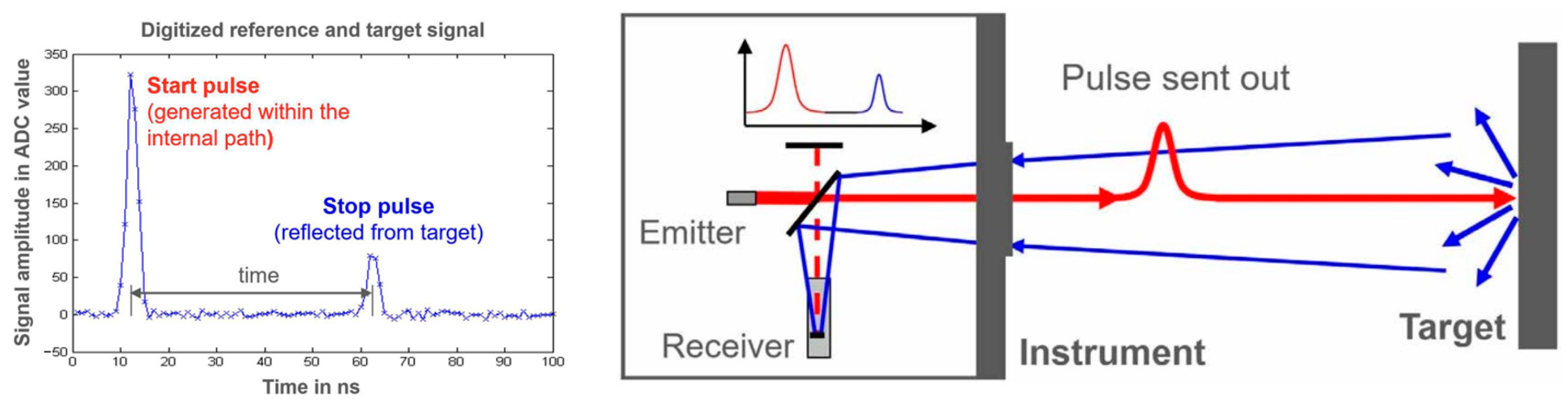
- Leica WFD—Wave Form Digitizer Technology White Paper. Available online: https://leica-geosystems.com/it-it/about-us/content-features/wave-form-digitizer-technology-white-paper (accessed on 9 January 2025).
- Russo, M.; Morlando, G.; Guidi, G. Low-cost characterization of 3D laser scanners. In Proceedings of the SPIE—The International Society for Optical Engineering, Videometrics IX, 6491, San Jose, CA, USA, 28 January–1 February 2007. [Google Scholar]
- Gruen, A.; Beyer, H.A. System Calibration Through Self-Calibration. In Calibration and Orientation of Cameras in Computer Vision; Grun, A., Huang, T.S., Eds.; Springer: Berlin, Germany, 2001; Volume 34, pp. 163–193. [Google Scholar]
- Luhmann, T.; Robson, S.; Kyle, S.; Boehm, J. Close-Range Photogrammetry and 3D Imaging; Walter de Gruyter GmbH: Berlin, Germany; Boston, MA, USA, 2023; pp. 154–158. [Google Scholar]
- Remondino, F.; Fraser, C.S. Digital camera calibration methods: Considerations and comparisons. Int. Arch. Photogramm. Remote Sens. Spat. Inf. Sci. 2006, 36, 266–272. [Google Scholar]
- Schönberger, J.L.; Frahm, J.M. Structure-from-Motion Revisited. In Proceedings of the Conference on Computer Vision and Pattern Recognition, Las Vegas, NV, USA, 27–30 June 2016; pp. 4104–4113. [Google Scholar]
- Brown, D.C. Close-Range Camera Calibration. Photogramm. Eng. 1971, 37, 855–866. [Google Scholar]
- Remondino, F.; Spera, M.; Nocerino, E.; Menna, F.; Nex, F. State of the art in high density image matching. Photogramm. Rec. 2014, 29, 144–166. [Google Scholar]
- Guidi, G.; Malik, U.S.; Micoli, L.L. Optimal Lateral Displacement in Automatic Close-Range Photogrammetry. Sensors 2020, 20, 6280. [Google Scholar] [CrossRef]
- Beraldin, J.A. Integration of Laser Scanning and Close-Range Photogrammetry—The Last Decade and Beyond. In Proceedings of the 20th ISPRS Congress, Istanbul, Turkey, 12–23 July 2004. [Google Scholar]
- Remondino, F.; El-Hakim, S. Image-based 3D modelling: A review. Photogramm. Rec. 2006, 21, 269–291. [Google Scholar] [CrossRef]
- Nocerino, E.; Menna, F.; Remondino, F. Accuracy of typical photogrammetric networks in cultural heritage 3D modeling projects. Int. Arch. Photogramm. Remote Sens. Spat. Inf. Sci. 2014, XL-5, 465–472. [Google Scholar] [CrossRef]
- Agisoft LCC Agisoft Metashape User Manual—Professional Edition, Version 2.1.1. Available online: https://www.agisoft.com/pdf/metashape-pro_2_1_en.pdf (accessed on 9 January 2025).
- CloudCompare. Available online: www.cloudcompare.org (accessed on 9 January 2025).
- Besl, P.J.; McKay, N.D. A Method for Registration of 3-D Shapes. IEEE Trans. Pattern Anal. Mach. Intell. 1992, 14, 239–256. [Google Scholar] [CrossRef]
- Masuda, T.; Sakaue, K.; Yokoya, N. Registration and Integration of Multiple Range Images for 3-D Model Construction. In Proceedings of the 13th International Conference on Pattern Recognition, Vienna, Austria, 25–29 August 1996; pp. 879–883. [Google Scholar]
- Unity Real-Time Development Platform. Available online: www.unity.com/ (accessed on 9 January 2025).
- Vasiljević, I.; Obradović, R.; Đurić, I.; Popkonstantinović, B.; Budak, I.; Kulić, L.; Milojević, Z. Copyright Protection of 3D Digitized Artistic Sculptures by Adding Unique Local Inconspicuous Errors by Sculptors. Appl. Sci. 2021, 11, 7481. [Google Scholar] [CrossRef]


| Technology | Focus | Resolution | Sensor Size | ISO Sensibility | Noise Level | Color Depth |
|---|---|---|---|---|---|---|
| 100 Megapixel BSI CMOS Sensor | Phase Detection Autofocus PDAF (97% coverage) | 100 megapixel (pixel pitch 3.78 μm) | 11,656 (W) × 8742 (H) pixel | 64–25,600 | 0.4 mm a 10 m | 16 bit |
| Focal Length | Equivalent Focal Length | Aperture Range | Angle of View diag/hor/vert | Minimum Distance Object to Image Plane |
|---|---|---|---|---|
| 120.0 mm | 95 mm | 3.5–45 | 26°/21°/16° | 430 mm |
| Technology | Framed Range | Accuracy | Lateral Resolution | 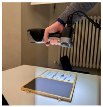 |
| 7 parallel infrared laser lines + VCSEL infrared structured light | 580 × 550 mm (DOF 720 mm with an optimal scanning distance of 400 mm) | 0.1 mm | 0.01 mm |
| Technology | Framed Range | Accuracy | Resolution | Precision | 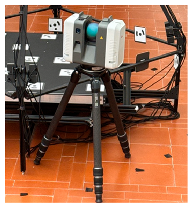 |
| High dynamic ToF with Wave Form Digitizer Technology (WFD) | 360° (H)–300° (V) | 1.9 mm at 10 m | 3 mm at 10 m | 0.4 mm at 10 m |
| Focal Length | Equivalent Focal Length | Aperture Range | Angle of View diag/hor/vert | Minimum Distance Object to Image Plane |  |
| 38.0 mm | 30 mm | 2.5–32 | 70°/59°/46° | 300 mm |
| Captured Area | 295 × 440 mm |
| Sampled points | 6,130,559 |
| Average distance between a fitted plane and point cloud | 0.000441619 mm |
| Standard deviation | 0.0172472 mm |
| Captured Area | 250 × 500 mm |
| Sampled points | 664,675 |
| Average distance between a fitted plane and point cloud | 0.374145 mm |
| Standard deviation | 0.313806 mm |
| Value | Error | f | Cx | Cy | b1 | b2 | k1 | k2 | k3 | p1 | p2 | |
|---|---|---|---|---|---|---|---|---|---|---|---|---|
| f | 10,228.5 | 0.64 | 1.00 | −0.07 | 0.05 | −0.90 | 0.04 | −0.18 | 0.19 | −0.18 | −0.11 | −0.09 |
| Cx | 8.87514 | 0.44 | - | 1.00 | −0.07 | 0.10 | 0.14 | 0.01 | −0.01 | 0.00 | 0.93 | −0.07 |
| Cy | −20.5956 | 0.53 | - | - | 1.00 | −0.21 | 0.08 | 0.03 | −0.03 | 0.03 | −0.09 | 0.72 |
| b1 | −10.4546 | 0.59 | - | - | - | 1.00 | −0.01 | 0.01 | −0.03 | 0.04 | 0.14 | 0.00 |
| b2 | −6.16297 | 0.23 | - | - | - | - | 1.00 | −0.01 | 0.01 | −0.00 | 0.05 | 0.04 |
| k1 | −0.015391 | 0.00023 | - | - | - | - | - | 1.00 | −0.97 | 0.93 | 0.02 | 0.03 |
| k2 | 0.0460376 | 0.0017 | - | - | - | - | - | - | 1.00 | −0.99 | −0.02 | −0.03 |
| k3 | −0.114143 | 0.0048 | - | - | - | - | - | - | - | 1.00 | 0.02 | 0.03 |
| p1 | 0.000138551 | 0.000014 | - | - | - | - | - | - | - | - | 1.00 | −0.07 |
| p2 | 0.000219159 | 0.000011 | - | - | - | - | - | - | - | - | - | 1.00 |
| ID | X | Y | Z |
|---|---|---|---|
| 1 | −112.1833981 | −265.6449903 | 1.1604001 |
| 2 | −356.9368841 | 27.3719204 | 1.1928803 |
| 3 | 218.4486223 | 167.6946044 | 0.7668501 |
| 4 | −83.5303045 | 335.2168791 | 0.8040630 |
| 5 | −356.2072197 | −267.7837971 | 1.4174284 |
| 6 | 422.8374003 | 36.3053955 | 0.8180338 |
| 7 | 418.5192553 | −267.5176537 | 0.7987372 |
| 8 | 172.0460260 | −268.9918738 | 1.0840074 |
| 9 | −166.6299110 | −121.8379844 | 1.2866903 |
| 10 | 20.7659104 | −72.1971757 | 0.9835656 |
| 11 | 219.4242678 | −120.2348847 | 0.8334230 |
| 12 | 21.4847097 | 100.0491205 | 0.8094964 |
| 13 | 175.3704988 | 336.8665062 | 0.7985485 |
| 14 | 421.7712423 | 327.9472855 | 1.4888459 |
| 15 | −357.4699748 | 331.4955047 | 0.9538767 |
| 16 | −163.2943198 | 169.2829513 | 0.7963140 |
| Agisoft Metashape Professional | Colmap | |
|---|---|---|
| Number of registered images | - | 132 |
| Number of tie points | - | 27,951 |
| Mean observations per image | - | 859,106 |
| Number of points in the dense cloud | 10,367,336 | - |
| RMS reprojection error | - | 0.485 px |
| Average distance of points | 0.5214 mm |
| Standard deviation | 0.77006 mm |
| PoI | X | Y | Z |
|---|---|---|---|
| Origin | 0 | 0 | 0 |
| Relio_1 | −646.79 | 3.0601 | 171.98 |
| Relio_2 | −3.6600 | 643.86 | 166.24 |
| Relio_3 | 641.34 | 0.3800 | 163.33 |
| Relio_4 | −5.1200 | −645.04 | 165.76 |
| Relio_5 | −474.21 | 2.6700 | 471.77 |
| Relio_6 | 0.1300 | 476.28 | 459.22 |
| Relio_7 | 466.87 | 0.0700 | 467.11 |
| Relio_8 | −5.3300 | −485.74 | 442.38 |
| Camera | 0.0600 | 0.2602 | 1542.48 |
| ID | X | Y | Z |
|---|---|---|---|
| 1 | −91.7384979 | −254.3196531 | 0.9266232 |
| 2 | −318.6724500 | 98.8737499 | 0.9983411 |
| 3 | 161.4589829 | 252.5450786 | 1.0497326 |
| 4 | 319.6547597 | −319.3383336 | 1.0325548 |
| 5 | −324.2391213 | −105.5458775 | 0.8632963 |
| 6 | 102.4372316 | −79.8087193 | 0.8986234 |
| 7 | −170.2707334 | 252.3647593 | 1.4474652 |
| 8 | −319.6547597 | 319.3383336 | 1.3325548 |
| 9 | 95.2218163 | 96.9329011 | 1.1688642 |
| 10 | 146.1604507 | −261.1907211 | 0.9117996 |
| 11 | −168.9669076 | −16.3564388 | 1.2615517 |
| 12 | 322.6046628 | 126.2068312 | 0.9887015 |
| 13 | −8.7779598 | 248.4658266 | 1.2592235 |
| 14 | −313.2096315 | −327.6061740 | 1.1325548 |
| 15 | 319.9531910 | 319.3383336 | 1.1325548 |
| 16 | 317.9581155 | −126.1577396 | 0.8518509 |
| Agisoft Metashape Professional | Colmap | |
|---|---|---|
| Number of registered images | 102 | |
| Number of tie points | 70.221 | |
| Mean observations per image | - | 1099.99 |
| Number of points in the dense cloud | 11,373,875 | - |
| RMS reprojection error | - | 0.465 px |
| Agisoft Metashape Professional | Colmap | |
|---|---|---|
| Number of registered images | - | 133 |
| Number of tie points | 118,213 | - |
| Mean observations per image | - | 2990.75 |
| Number of points in the dense cloud | 12,054,708 | - |
| RMS reprojection error | - | 0.499 px |
| Average distance of points | 0.5218 mm |
| Standard deviation | 0.79912 mm |
| Average distance of points | 0.4924 mm |
| Standard deviation | 0.69464 mm |
| PoI | X | Y | Z |
|---|---|---|---|
| Origin | 0 | 0 | 0 |
| Relio_1 | 10.7631 | −225.7121 | 601.7119 |
| Relio_2 | 605.4825 | −226.7232 | −4.3642 |
| Relio_3 | 7.4924 | −239.9226 | −609.6511 |
| Relio_4 | −603.3234 | −230.8313 | 1.2631 |
| Relio_5 | 0.3228 | −537.4174 | 472.5922 |
| Relio_6 | 461.0301 | −537.3921 | 8.2132 |
| Relio_7 | 1.5820 | −541.6323 | −456.7912 |
| Relio_8 | −461.62 | −537.2876 | 8.1521 |
| Camera | 0.0323 | −1543.8149 | 0.0101 |
| PoI | X | Y | Z |
|---|---|---|---|
| Origin | 0 | 0 | 0 |
| Relio_1 | −1.8714 | −235.8112 | 611.5131 |
| Relio_2 | 607.6222 | −225.0312 | −0.5913 |
| Relio_3 | 11.6712 | −238.3611 | −624.8112 |
| Relio_4 | −589.1021 | −223.7463 | −2.9221 |
| Relio_5 | −2.9265 | −543.3825 | 469.5811 |
| Relio_6 | 460.6141 | −538.2921 | 8.1423 |
| Relio_7 | 4.6122 | −539.5241 | −463.3921 |
| Relio_8 | −458.0721 | −533.0126 | 8.1811 |
| Camera | 0.04 | −1543.3821 | 0.1712 |
| PoI | X | Y | Z | Euclidean Distance |
|---|---|---|---|---|
| Origin | 0 | 0 | 0 | 0 |
| Relio_1 | −12.6345 | −10.0991 | 9.8012 | 18.9125 |
| Relio_2 | 2.1397 | 1.6920 | 3.7729 | 4.6557 |
| Relio_3 | 4.1788 | 1.5615 | −15.1601 | 15.8023 |
| Relio_4 | 14.2213 | 7.0850 | −4.1852 | 16.4304 |
| Relio_5 | −3.2493 | −5.9651 | −3.0111 | 7.4301 |
| Relio_6 | −0.4160 | −0.9000 | −0.0709 | 0.9940 |
| Relio_7 | 3.0302 | 2.1082 | −6.6009 | 7.5629 |
| Relio_8 | 3.5479 | 4.2750 | 0.0290 | 5.5555 |
| Camera | 0.0077 | 0.4328 | 0.1611 | 0.4618 |
Disclaimer/Publisher’s Note: The statements, opinions and data contained in all publications are solely those of the individual author(s) and contributor(s) and not of MDPI and/or the editor(s). MDPI and/or the editor(s) disclaim responsibility for any injury to people or property resulting from any ideas, methods, instructions or products referred to in the content. |
© 2025 by the authors. Licensee MDPI, Basel, Switzerland. This article is an open access article distributed under the terms and conditions of the Creative Commons Attribution (CC BY) license (https://creativecommons.org/licenses/by/4.0/).
Share and Cite
Gaiani, M.; Angeletti, E.; Garagnani, S. Photometric Stereo Techniques for the 3D Reconstruction of Paintings and Drawings Through the Measurement of Custom-Built Repro Stands. Heritage 2025, 8, 129. https://doi.org/10.3390/heritage8040129
Gaiani M, Angeletti E, Garagnani S. Photometric Stereo Techniques for the 3D Reconstruction of Paintings and Drawings Through the Measurement of Custom-Built Repro Stands. Heritage. 2025; 8(4):129. https://doi.org/10.3390/heritage8040129
Chicago/Turabian StyleGaiani, Marco, Elisa Angeletti, and Simone Garagnani. 2025. "Photometric Stereo Techniques for the 3D Reconstruction of Paintings and Drawings Through the Measurement of Custom-Built Repro Stands" Heritage 8, no. 4: 129. https://doi.org/10.3390/heritage8040129
APA StyleGaiani, M., Angeletti, E., & Garagnani, S. (2025). Photometric Stereo Techniques for the 3D Reconstruction of Paintings and Drawings Through the Measurement of Custom-Built Repro Stands. Heritage, 8(4), 129. https://doi.org/10.3390/heritage8040129