Abstract
Quantifying bolt tension and ensuring that bolts are appropriately tightened for large-scale civil infrastructures are crucial. This study investigated the feasibility of employing the surface acoustic wave (SAW) for quantifying the bolt tension via finite element modeling. The central hypothesis is that the real area of contact in a bolted joint increases as the tension or preload is increased, causing an acoustical signature change. The experimentally verified 3-D simulations were carried out in two steps: A preload was first applied to the bolt body to simulate the realistic behavior of bolted joint; and the SAW propagation was then excited on the top surface of the plate to reflect from the bolted joint. The bolt tension value was varied between 4 and 24 kN (properly tightened bolt) in the steps of 4 kN to study the effect of the bolt tension. The results indicate an increased reflected wave amplitude and a gradual phase shift, up to 0.5 µs, as the bolt tension increased. Furthermore, the result shows that the distance between the first reflected wave and the source becomes shorter as the preload increases, as hypothesized. A 1.9 mm difference in the distance between the maximum and minimum preload was observed. As part of this study, the simulation results were also compared with the experimental results, and a good agreement between the simulation and experiments was demonstrated.
1. Introduction
The health of bolted joints depends mainly on the status of the threaded fastener since the fastener is responsible for holding two structural components together. Therefore, any failure occurring in the fasteners may lead to a catastrophic failure in the entire engineering structure or machine. One common problem that bolted joints commonly experience is the loosening of a bolt, indicating a decrease in the tension force on the bolt, which is equivalent to the clamping force on the joints. A bolt loosening can take place due to various causes such as plastic deformation of the bolted joint components, the slip between the joint parts, and wear of joint parts [1].
The bolt tension should be monitored periodically to prevent failure in bolted joints due to bolt loosening. Various useful techniques were developed over the last few decades to quantify the bolt tension. These techniques can be classified into two main categories: the techniques necessitating bolt contact, and the contactless bolt measurement techniques. The torque wrench technique is the most common method to estimate the bolt tension through applying a wide range of torque values to clamp the bolt. However, the measurement accuracy of this standard methodology can be low due to disregarding the friction between the bolt thread and the nut [2,3]. Another example of a measurement technique that operates by contacting the bolt is the acoustoelastic effect based method [4]. This technique requires attaching an ultrasonic transducer to the bolt head to generate a combination of longitudinal and transverse ultrasonic waves that travel to the bolt end and then reflects to the transducer. By processing the time of flight (TOF) of wave data, the effective bolt length can be estimated which then enables the measurement of the tension force on the bolt based on the acoustoelastic constant of the material.
Among the contactless bolt tension quantification techniques, one standard methodology is the piezoelectric active sensing method [5]. In this technique, two piezoelectric patches are attached to the top surfaces of both plates of bolted joints. The role of the first piezoelectric transducer is to generate the ultrasonic wave that travels through the interface contact between the two plates, while the second piezoelectric transducer is responsible for receiving the propagated wave. The energy of the received wave signal depends on the clamping force at the interface, which is then analyzed to quantify the bolt tension and identify bolt loosening.
In our previous study, the authors experimentally investigated an alternative method to quantify bolt tension without contacting the bolt using a synthetic phased-array surface acoustic wave (SAW) operating at 5 MHz [6]. The SAWs were generated by a linear transducer array that is located only on one surface of bolted joints. The central hypothesis was that the real area of contact in a bolted joint increases as the tension or preload is increased, which causes an acoustical signature that can be easily measured with the SAWs synthetic phased array [6]. The phased array method is utilized to acquire high-resolution ultrasonic images. The reflection of SAWs created by the real contact area between the bolt head and the plate surface is then used to quantify the tension on the bolt. It was observed that the distance between the transducer and the reflected wave shortens as the bolt tension increases.
This study takes the investigation of this technique to the next level by exploring the use of ultrasonic waves to quantify the bolt tension via simulating the surface acoustic wave (SAW) propagation over the bolted joint surface. The 3D simulations were carried out by a commercially available Finite Element modeling software (ANSYS 18.1). The simulations were conducted in two main steps: First, applying a preload to the bolt body to simulate the real behavior of bolted joint under the real conditions; second, exciting the SAWs signal on the top surface of the bolted joint to reflect from the interface between the bolt head and the top surface. For a thorough investigation, six separate simulation studies were carried out. Each simulation has different preload values to understand the influence of preload on the incident wave amplitude. The preload value was varied between 4 and 24 kN in the steps of 4 kN.
2. Fundamentals of Ultrasonic Waves
The ultrasonic waves have been widely utilized in nondestructive testing and structural health monitoring due to their abilities to detect defects as well as to inspect large engineering structures. The ultrasonic waves can exist in various modes and frequencies and can travel a long distance in both flat and curved structures with low energy loss [7,8]. The ultrasonic elastic waves in solids can be classified into bulk elastic waves and guided elastic waves. Unlike bulk ultrasonic waves, guided elastic waves are dispersive, which indicates that the phase velocity of wave relies on their frequency. As a result, the group velocity of bulk waves is not equal to their phase velocity. The guided ultrasonic elastic waves can propagate in solids as elastic surface waves (Rayleigh wave) which represents a combination of shear and longitudinal waves, Lamb waves, or shear horizontal waves. Lamb waves are the most complicated type of all since they have two different modes, symmetric or antisymmetric. Lamb waves can be excited in thin plates (finite plates), where the plate thickness is much smaller than the wavelength. The surface waves propagate along the free surface of the solid where the plate thickness is large compared to the wavelength, and the surface particles move in an elliptical path. The amplitude of the Rayleigh wave decays in the direction of the plate thickness [7,8,9].
In a perfectly elastic isotropic solid, the longitudinal (CL) and shear velocity (Cs) are related to the material properties which can be expressed in Equations (1) and (2). The approximation of the Rayleigh wave velocity (CR), which depends on the shear wave speed and the material properties, can be expressed in Equation (3) [7]:
where E is the elastic modulus, ρ is the density, µ is the modulus of rigidity and ν is the Poisson ratio.
3. Simulation Work
3.1. Initial Simulation Studies
In order to understand and verify the behavior of SAW propagation on a flat plate, a 40 mm thick, 130 mm long, and 100 mm wide plate without any holes or bolts was simulated in a commercially available finite element software, (ANSYS Inc., Release18.1, Canonsburg, PA, USA). The plate is taken as steel with Young’s modulus of 200 Gpa, Poisson’s ratio of 0.33, shear modules of 76.9 Gpa, and density of 7850 kg/m3 [10]. For more consistent meshing control, the top surface was sliced to 3 mm in depth, and then the two slices were consolidated with a bonded contact to be as one part [11]. The incorporation of slices not only allows the localization of a dense mesh for the top surface and less dense mesh along with the remaining thickness of the plate, but it also allows for reducing the computational time to solve the finite element (FE) model since the number of nodes is significantly decreased. Initially, a single nodal point on the upper left surface was selected to represent a single transducer to excite the wave. However, the authors observed that the generated wave is circular which leads to undesirable and non-realistic reflections from the plate sides. These reflections interacted with the incident wave, making the results more complicated to analyze. For this reason, twelve evenly distributed point sources near the upper left end of the plate were selected to excite SAW where each point source represents a single transducer. The generated wave is a straight line when it leaves the source and becomes a curved line as it travels far from the source, similar to our experimental observations. However, large plates necessitate additional point sources to excite a particular wave mode and reduce the noise level [12]. In addition to twelve transmitting point sources, evenly spaced three receivers were introduced to the model. These are nodal points that are located at the top surface of the plate. Both the left and right end of the plate had a fixed boundary condition. Figure 1 illustrates the geometrical details and boundary conditions of the initial verification studies.
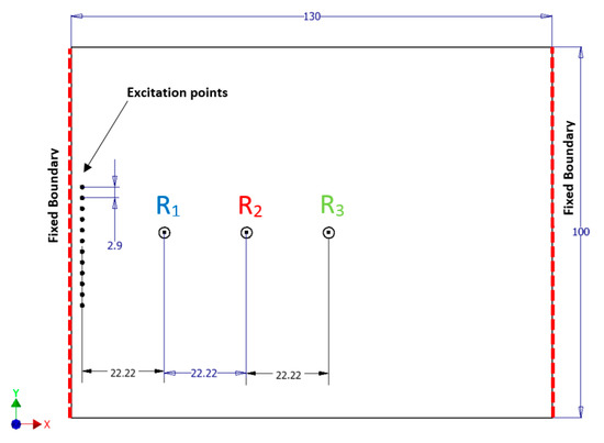
Figure 1.
Schematic representation of the top surface of the plate, including the locations of the three receivers and twelve transmitting point sources. All dimensions are in mm.
The main goal of the initial simulation studies was to obtain the Rayleigh surface wave velocities at each receiver and validate them against the theoretical value reported elsewhere. This was achieved by obtaining the zero-crossing time of the wave at each receiver. Another goal of the initial simulation studies was to obtain the length of time that the surface wave needed to travel from the wave source to the right end of the plate and verify it with the theoretical time. By knowing the entire time needed for the input signal, unwanted reflections from the far end of the plate can be avoided, and the computational time needed can be reduced [13]. Most FEA commercial software lacks a perfectly matched layer (PML), which is essential for absorbing or attenuating propagating waves and hence preventing them from being reflected in the study area.
3.2. Preload Analysis
The bolt pretension simulation study aims to replicate the real behavior of bolted joints after applying a particular preload value on the bolt body. Typically, the preload on a bolt occurs when applying the torque to either the bolt head or the nut. There is a directly proportional correlation between the torque and preload on a bolt: The higher the applied torque to bolt, the higher the preload is on the bolt and vice versa. However, the preload magnitude not only depends on the applied torque, but also on other important factors such as the bolt diameter, the friction coefficient between the bolt body and plate surfaces, and bolt thread geometry [14]. The preload and torque relationship is described by the following equation:
where T is the applied torque, F is the preload, d is the bolt diameter, and K is the nut factor. The estimated range of K value is 0.10~0.2 depending on the type of lubricant, size of bolt, and bolt material [14]. In this study, K = 0.18 was utilized [6]. To avoid the plastic deformation on the bolt, the applied preload on a bolt should not exceed the maximum allowable limit. Thus, the maximum allowable preload can be estimated using Equation [14]:
where Fi is the maximum allowable preload (proof load), At is tensile stress area which is a function of thread pitch, Sy is yield strength of the bolt, and d is the nominal bolt diameter. In this study, a standard medium carbon steel bolt and nut with 10 mm nominal diameter were imported from the commercially available CAD software library, Inventor Autodesk 2018. Based on the bolt material and nominal diameter, the value of Sy and At are 640 N/mm2 [15] and 57.1 mm2 respectively. After substituting all values into Equation (5), the maximum allowable preload that bolt can withstand is obtained as 23.3 kN, and it is rounded up to 24 kN. By substituting this value into Equation (4), the maximum allowable torque on bolt is 43 N.m. For comparison purposes, six values of preload were utilized in this study. The preload values varied between 4 and 24 kN in the steps of 4 kN.
To properly perform a bolt pretention analysis in ANSYS, the type of contact between bolted joint parts should be carefully selected. These contacts represent how each part moves relative to other parts. The coefficient of friction, Cf , is assumed to be 0.2 for all frictional contact type [16]. Table 1 shows the details of the contacts used in this study.

Table 1.
Contacts set-up between the bolt and plate.
ANSYS 18.1 offers the bolt pretension feature as a boundary condition that applies to both static and transient structural analyses. This boundary condition is essential for obtaining the real behavior of bolt in joints since it offers five different types of loading on the bolt body. These types of loading are load, adjustment, lock, open, and increment. In the structural analysis, this study utilized two steps in the boundary condition. The first step was to simulate the assembly of joints by applying a load on the bolt body as a preload. The second step was to simulate the real behavior of a joint under real conditions by applying a lock on the bolt [17]. From this analysis, the adjustment value (the change in the bolt length) was obtained. This is used in the first step of the transient analysis.
3.3. Transient Simulations
The 3-D transient simulations were performed in two main steps: First, the adjustment value on the bolt body was applied, followed by locking the bolt to simulate the bolted joints behavior; then, applying a displacement load that acts perpendicular to the top surface of the plate at the twelve point sources. Before running the simulation, the basic parameters of a continuous ultrasound wave were defined for simulating the real behavior of waves in a solid material. The first parameter is the Rayleigh wave propagation speed, CR, that mainly depends on the mechanical properties of the material, and it can be estimated using Equation (3). The second parameter is the wavelength (λ) which is equal to the ratio of the ultrasonic wave speed (CR) to the frequency (ƒ) in a perfectly elastic material . By utilizing the material properties for steel and Equation (3), the Rayleigh wave speed (CR) was found to be 2917.58 m/s. The corresponding wavelength for this wave speed and the central frequency of interest (100 kHz) was obtained as 29.1 mm, which was rounded to 29 mm.
In order to achieve an accurate solution of ultrasound wave propagation using the finite element analysis (FEA), an adequate temporal and spatial discretization is required. A precise time step, Δt, is needed to model the temporal behavior of the wave propagation and should be smaller than the critical time step of the studied phenomena. A proper element size should be selected for solving the wave propagation spatially. In general, the smaller the time step and element size, the higher is the solution accuracy. Although the solution accuracy improves with a smaller value of the time step and element size, unnecessarily small values necessitate significantly increased computational time. For these reasons, it is generally recommended to use 8 to 20 elements per wavelength [13,18,19], and 10 to 20 points per cycle of the highest frequency for the time step [13,20]. In this study, the time step and the element size were evaluated using Equations (6) and (7).
where fmax is the maximum frequency, le is the element size, and λmin is the shortest wavelength. In the case of this simulation, the wavelength was found to be 29 mm. Thus, the estimated values for time step and element size were obtained from Equations (6) and (7) as 0.5 µs and 2.9 mm, respectively.
In a finite element analysis, a surface acoustic wave can be produced in an elastic solid by either a localized impact on the surface or by a piezoelectric transducer. The loading condition of the elastic wave excitation in FEA can be achieved either by applying a force on the surface [21,22] or a nodal displacement [13,23]. In a real-life application, the surface acoustic wave is excited on the test specimen by using an angle beam transducer, a normal beam transducer, or a comb transducer. The angle beam transducer is the most efficient technique for producing the surface waves since it requires only one angle for all frequencies. The wedge material of an angle beam transducer with an incident angle of 58.42° produces surface waves which propagate with an angle of 90° on the surface of the test specimen(steel) [24]. Here, for excitation the SAW, a displacement load in Z-direction (perpendicular to the wave propagation direction) at 12 excitation source points was applied. These are located on the top left surface. The loading function was based on a 100-kHz 2-cycle Hanning- window tone burst that was obtained from Equation (8) [7]:
where ƒ is the modulation frequency, t is the time, TH is the number of cycles divided by the frequency. Substituting the time step of 0.5 µs, the frequency of 100 kHz, and several cycles of 2 into the Equation (8), the time function of the input signal is obtained, as shown in Figure 2. Figure 2a illustrates that the input signal completes two cycles in 20 µs, and after this time, the displacement should be set to be zero. The total duration time of the simulation, 60 µs, was selected based on the initial simulation results that showed the incident wave reaching the far end of the plate at the time of 60 µs. A 42 ns (0.042 µs) time step was taken between 20 and 60 µs to record additional data of the wave amplitude; hence, an accurate comparison can be achieved.
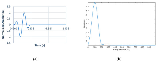
Figure 2.
(a) The time domain of the excitation signal; (b) the frequency spectrum of the excitation signal obtained by FFT.
The mesh parameters were selected to characterize the surface wave propagation on the plate surface accurately. In all sets of simulations, the hexahedral element type and tetrahedron element type were chosen for the plate and the bolt respectively. The mesh element size, 2.9 mm, was evaluated using Equation (7) to solve the wave propagation spatially. The mesh quality is a critical aspect in computing and solving the FEA model correctly, and it should be analyzed in each simulation. There are three key mesh statistics can be checked in ANSYS, which are skewness, orthogonal quality, and element quality. In this study, the average value of orthogonal quality, element quality, and skewness were 0.9, 0.84, and 0.1, respectively. The excellent values should be 0.95 for the average orthogonal quality, and 0.3 for element quality, and be less than 0.25 for the average skewness [11]. Figure 3a illustrates the geometry details and Figure 3b shows the top view of the top surface of the plate including the location of the receivers, the excitation points, and the reflected wave propagation path.
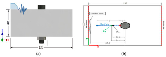
Figure 3.
(a) Schematic representation of the bolted joint geometry; (b) the top view of the geometry, including the receiver locations and the reflected wave propagation path. All dimensions are in mm.
4. Results and Discussion
4.1. Verification Studies
The goal of initial verification studies is to simulate the SAW propagation on a plate without a hole or a bolt and then verify the SAW propagation velocity and its central frequency. For verification purposes, three receivers along the direction of wave propagation (X-axis) were located on the plate surface, and the displacement response of each receiver was recorded. The distance between each receiver (R1, R2, and R3 as illustrated in Figure 1) and the SAW source are 20.22, 40.44, and 60.667 mm, respectively. Figure 4a shows the response of each receiver (displacement in the Z direction) and the time of zero-crossing for the three signals to verify the phase velocity based on a zero-crossing algorithm using Equation (9) [25,26].
where is the distance between two receivers and is the delay time calculated for the zero-crossing point in the same phase for the two signals, as illustrated in Figure 4. The results of phase velocity that are obtained from Equation (10) and the theoretical phase velocity of the incident signal calculated from Equation (3) are listed in Table 2. It can be observed from the Table 2 that the error between the theoretical and simulated phase velocity is reasonably small (less than 0.4% for all cases studied). Furthermore, to verify the frequency of SAW, fast Fourier transform (FFT) of the obtained signal was taken to convert the time domain of the signal into a frequency domain [27]. Figure 4b illustrates the frequency domain of the signal response at R3. It is worth noting that the central frequency is almost 100 kHz, which is in a good agreement with the central frequency of the incident wave.
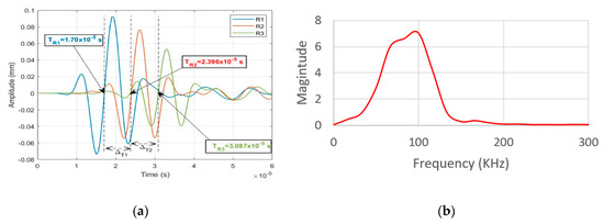
Figure 4.
(a) Displacement responses in Z-axis for the three receivers R1, R2, and R3 as illustrated in Figure 1; (b) Frequency spectrum for R3 in Z-axis obtained by FFT.
Table 2.
Phase Velocity Verification.
4.2. A Comparison Between No Hole and Fully-Loosened Bolt
As discussed in the previous section, two sets of simulation studies were conducted: (a) A plate with no hole or bolt; (b) a bolted plate having all components of the bolted joint. In the bolted plate simulation, the four contacts between the bolt and plate were removed to simulate the fully loosen bolt case. Figure 5 illustrates the displacement response in the Z-axis for both cases under the same boundary conditions. These responses were recorded using one receiver near the SAW source. It can be observed in Figure 5b that there is a noticeable difference between the two amplitudes, particularly between the time of 40 and 60 µs due to the reflected wave propagation from the hole toward the source in case of the entirely-loosened bolt. Expectedly, this reflection is not observed for the plate without the hole in the design.
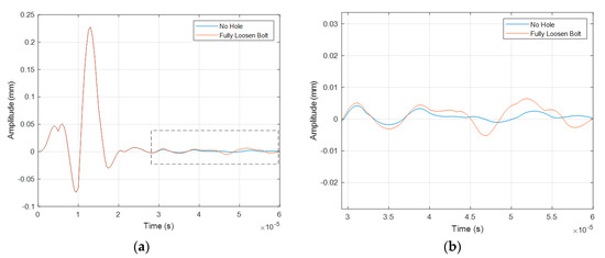
Figure 5.
(a) Displacement responses in Z-axis for no hole and fully-loosened bolt cases; (b) Zoomed-in view between the time of 30 and 60 µs for no hole and fully-loosened bolt cases.
4.3. Detection of Wave Reflection
Based on the visual observation of incident wave which propagates in the positive x-direction after the excitation, the major reflection, which propagates in the opposite direction of the original wave propagation (−X direction), occurs when the incident wave completely passes the bolt head approximately at the time stamp of 42 µs. However, detecting the exact time of the major reflection in the time history of the wave signal for any receiver requires placing one additional receiver -R4- before the receiver -R5- with a very short distance between the two receivers as illustrated in Figure 3. The inclusion of the additional receiver in the analysis not only enables distinguishing between the incident wave and the reflected wave from the bolt, but also enables implementing an accurate comparison when different preload values are applied to the bolt. Figure 6 shows the time history of the wave at the two receivers. It can be noted that between time 15 and 46 µs, the wave passes the R5 after passing the R4. After 46 µs the wave passes R5 earlier than R4, which indicates that the wave is traveling in the opposite direction (due to reflection). It can also be observed that there is a slight increase in the amplitude of the primary receiver at time 35 µs, which might be due to the reflection from the bolt which adds with the incoming wave constructively.
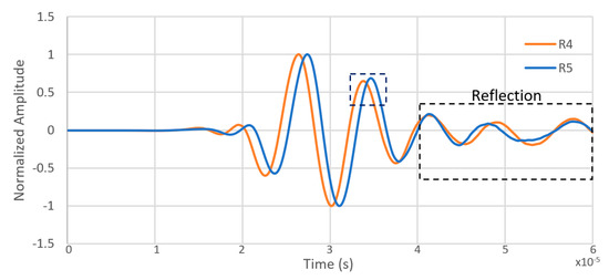
Figure 6.
Time history of the 4 kN signal that passes two neighboring receivers which are located before the bolt along the bolt center.
4.4. Particle Motion Along the Reflected Wave Propagation Path
The goal of the reflected wave particle motion investigation is to understand the wave reflection behavior with varying the preload on the bolt. As previously discussed, the major reflection takes place after time 42 µs. Therefore, this study created a 41 mm-long path. This path is located between the bolt and the source, consisting of 50 segments as shown in Figure 3b. The direction of this path is in the negative X-direction (reflected wave direction). The particle movement of the path in Z-direction for the five preload values was recorded from time 42 to 50 µs. Figure 7a shows the wave patterns reflected from the bolt at the time stamp of 46 μs. The displacement of the path at 46 µs was chosen for a better illustration of how the reflection varies as the preload value increases, as shown in Figure 7b. It can be observed from this figure that as the preload increases, the width of the reflection wave increased. It can also be observed that the reflection amplitude increases as the preload increases. There are four zero-crossing points along this path. The last zero-crossing point was chosen for comparison as it was the nearest point to the source. The distance of zero-crossing from the source for each preload is listed in Table 3. It can be observed that the zero-crossing of the higher preload of 24 kN has the shortest distance to the source, while the lower preload of 4 kN has the longest distance to the source. The difference in the distance between the lower and higher preload is approximately 1.9 mm. Figure 7c illustrates the average of the reflected wave amplitude between 42 and 50 µs along this path. It can be observed that the reflected wave associated with the higher preload has a higher amplitude average as the wave approaches the source. Table 3 also shows that the relationship between the reflection location and the preload is nonlinear as has been predicted by our earlier study [6]. Furthermore, a slight difference in the wavelength was observed in all five preload cases studied as shown in Table 3. Estimating the location of the first reflected wave has the potential to quantify the bolt tension.

Figure 7.
(a) The reflected waves from the bolt at time 46 µs; (b) The displacement in Z-direction along the reflected wave path at time 46 µs before the bolt; (c) The average displacement in Z-direction along the path between time 42 and 50 µs.
Table 3.
The distance of zero-crossing of each preload from the source and the corresponding wavelength. All dimensions in mm.
4.5. Time History of the Reflected Wave Near the Bolt
A comparison of varying the preload on the SAW propagation and reflection wave characteristics involves three necessary steps: (1) Recording the time history of the signal for each preload at the receiver -R5-, as illustrated in Figure 3b; (2) locating the reflection zone which was found to be after 42 µs; (3) measuring the difference using one preload case as a reference. Figure 8 shows the results of the three steps followed to investigate the effect of preload on wave propagation and reflection. It can be observed from Figure 8b that as the preload increases, the reflection amplitude increases. For this reason, the 4 kN case was taken as a reference for measuring the difference in the third step. It can also be noted that the phase of reflection wave shifts to the left as the preload increases, particularly at 46 µs. As a result, the peak amplitude of a higher preload occurs earlier than the lower preload, as was also observed in our earlier study [6]. The most considerable difference in time, 0.5 µs, exists between the higher and the lower preload. Figure 8c shows the amplitude difference from 40 to 60 µs, which is obtained from Equation (10)
where Ai is the amplitude of each preload, A4kN the reference amplitude (4 kN). It can be noted in Figure 8c that the maximum difference is found at time 46 µs, where the phase shifting of reflected wave occurs.
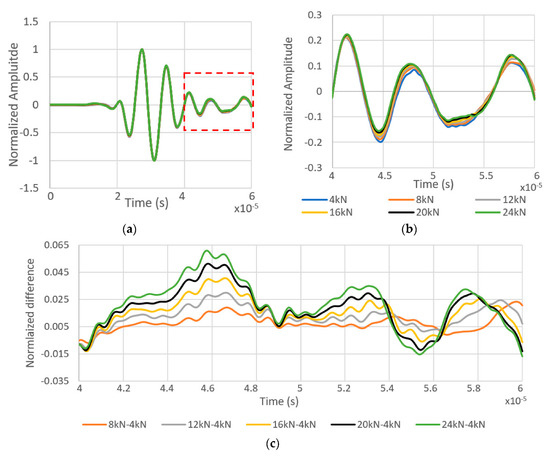
Figure 8.
(a) Time history of the propagating wave for all preload values; (b) Zoomed-in view of the reflection zone, located between 40 and 60 µs; (c) The differential representation of all preload cases with 4 kN case as the reference.
4.6. Simulation and Experimental Comparison
In our previous experimental study, the authors employed a 5 MHz ultrasonic transducer which was connected to a judiciously designed ultrasonic wedge to create surface waves propagating on the steel test specimen [6]. In order to obtain a higher resolution ultrasonic image, a synthetic phased array system was utilized. This system is simply formed by precisely moving the transducer linearly with a known pitch. The synthetic phased array system simulated a total of 50 elements in an array which was aimed to generate an acoustic beam. The bolted joints used in the experimental setup were a 12.7 mm thick 1018 steel plate, a 6.4 mm grade 8 bolt and a 19 mm stainless steel washer. The transducer was placed on the top surface of 1018 steel bolted joint from a distance of 29 mm from the bolt. During the experiments, five bolt tension values, similar to those presented in this study, were applied to the bolt for comparison. The bolt tension values are indirectly related to the applied torque as expressed in Equations 4 and 5. By analyzing the reconstructed ultrasonic images of SAWs for the different torque values, it was observed that as the applied torque increased, the distance of the first reflected wave from the bolted joint received by the transducer decreased. It should be highlighted that the same finding was observed in this simulation study presented here, as discussed in Section 4.4. Figure 9 illustrates the experimentally obtained distance of the first reflected wave from the transducer as a function of the applied torque. As shown in Figure 9, the longest distance of 27.9 mm observed corresponds to the lowest torque value (3.61 N.m) from the transducer, while the shortest distance of 27 mm is for a torque value of 10.31 N.m [6].
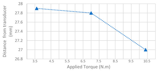
Figure 9.
The experimentally obtained distance of the first reflected wave from the transducer as a function of the applied torque.
In order to make a fair comparison between the simulation and experiment results, three torque values were normalized to the maximum applied torque for each case. For instance, the three selected torque values from the experiment are 3.61, 7, and 10.39 N.m. Normalizing these values to the maximum torque applied (10.39 N.m), resulted in 34%, 67%, and 100%. The three equivalent torque values from the simulation that lead to the same percentages are 14.4, 28.8, and 43.3 N.m. The simulated and experimentally observed shift from the maximum allowable torque are listed in Table 4. The values in Table 4 are obtained by subtracting the positions of first reflected wave for each applied torque that are shown in Table 3 and Figure 9 from the position of the first reflected wave associated with the maximum torque. It can be observed that there is an excellent agreement between the simulation and the experimental results with just a few millimeter differences between the two studies. It should be pointed out that the discrepancy between the simulation and experiment results can be due to several factors, such as the difference in the wave frequency studied, the bolt size, the bolt material, or the plate thickness.
Table 4.
The simulated and experimentally shift from the maximum allowable torque.
5. Conclusions
In this study, the effect of varying bolt tension on SAW was simulated via the commercially available finite element program, ANSYS 18.1. The study investigated the SAW reflection caused by the real contact area, which is located at the interface between the bolt head and plate surface. To ensure the validity of the FEA model developed, the phase velocity of the incident wave (SAW) and frequency were simulated and then compared with the theoretical values. The error in the phase velocity and frequency were 0.4% and negligible, respectively. The results show a clear trend of an increase in the reflected wave amplitude as the bolt tension are varied from 4 to 24 kN with a slight phase shifting of 0.5 µs. The results further show that as the bolt tension increases, the distance of the first reflected wave to the source becomes shorter. This was measured based on the nearest zero-crossing point to the source. The most significant difference in distance, 1.9 mm, was observed between 4 and 24 kN. Most importantly, the results also indicate that the bolt tension can be reliably quantified based on the location of the first reflected wave. The simulation results show an excellent agreement with the experiment results. The results presented here have the potential to significantly impact bolt tension quantifying and ensuring that all bolts are properly tightened for a large engineering structure or a machine.
Author Contributions
Investigation, H.A. and R.G.; methodology, R.G.; project administration, R.G.; resources, R.G.; supervision, R.G.; writing—original draft, H.A.; writing—review & editing, R.G.
Acknowledgments
The authors gratefully acknowledge the Research Computing Department at the University of South Florida for providing the computer resources which facilitate conducting the simulation in this paper.
Conflicts of Interest
The authors declare no conflicts of interest.
References
- Sakai, T. Bolted Joint Engineering: Fundamentals and Applications; Beuth Verlag: Berlin, Germany, 2008. [Google Scholar]
- Jhang, K.-Y.; Quan, H.-H.; Ha, J.; Kim, N.-Y. Estimation of clamping force in high-tension bolts through ultrasonic velocity measurement. Ultrasonics 2006, 44, e1339–e1342. [Google Scholar] [CrossRef] [PubMed]
- Wang, T.; Song, G.; Liu, S.; Li, Y.; Xiao, H. Review of bolted connection monitoring. Int. J. Distrib. Sens. Netw. 2013, 9, 871213. [Google Scholar] [CrossRef]
- Chaki, S.; Corneloup, G.; Lillamand, I.; Walaszek, H. Combination of longitudinal and transverse ultrasonic waves for in situ control of the tightening of bolts. J. Press. Vessel Technol. 2007, 129, 383–390. [Google Scholar] [CrossRef]
- Wang, T.; Song, G.; Wang, Z.; Li, Y. Proof-of-concept study of monitoring bolt connection status using a piezoelectric based active sensing method. Smart Mater. Struct. 2013, 22, 087001. [Google Scholar] [CrossRef]
- Martinez, J.; Sisman, A.; Onen, O.; Velasquez, D.; Guldiken, R. A synthetic phased array surface acoustic wave sensor for quantifying bolt tension. Sensors 2012, 12, 12265–12278. [Google Scholar] [CrossRef]
- Giurgiutiu, V. Structural Health Monitoring with Piezoelectric Wafer Active Sensors: With Piezoelectric Wafer Active Sensors; Elsevier: Amsterdam, The Netherlands, 2007. [Google Scholar]
- Rose, J.L. Ultrasonic Guided Waves in Solid Media; Cambridge University Press: Cambridge, UK, 2014. [Google Scholar]
- White, R.M. Surface elastic waves. Proc. IEEE 1970, 58, 1238–1276. [Google Scholar] [CrossRef]
- ANSYS®. Academic Research Mechanical Release 18.1, Static Structural, Engineering Data; ANSYS, Inc.: Canonsburg, PA, USA, 2019. [Google Scholar]
- Padilla, S.; Tufekcioglu, E.; Guldiken, R. Simulation and verification of polydimethylsiloxane (PDMS) channels on acoustic microfluidic devices. Microsyst. Technol. 2018, 24, 3503–3512. [Google Scholar] [CrossRef]
- Duan, W.; Niu, X.; Gan, T.-H.; Kanfoud, J.; Chen, H.-P. A Numerical Study on the Excitation of Guided Waves in Rectangular Plates Using Multiple Point Sources. Metals 2017, 7, 552. [Google Scholar] [CrossRef]
- Moser, F.; Jacobs, L.J.; Qu, J. Modeling elastic wave propagation in waveguides with the finite element method. NDT E Int. 1999, 32, 225–234. [Google Scholar] [CrossRef]
- Budynas, R.G.; Nisbett, J.K. Shigley’s Mechanical Engineering Design; McGraw-Hill: New York, NY, USA, 2008; Volume 8. [Google Scholar]
- Fastenal Technical Reference Guide. Available online: https://www.fastenal.com/content/documents/FastenalTechnicalReferenceGuide.pdf. (accessed on 13 March 2019).
- Vandermaat, D. Factors Affecting Pre-Tension and Load Carrying Capacity in Rockbolts—A Review of Fastener Design. In Proceedings of the 18th Coal Operators’ Conference, Wollongong, Australia, 7–8 February 2018. [Google Scholar]
- ANSYS®. Academic Research Mechanical, Products/Structures/Strength Analysis/Simulating Bolted Assemblies; ANSYS Inc.: Canonsburg, PA, USA, 2019; Available online: https://www.ansys.com/products/structures/strength-analysis/simulating-bolted-assemblies (accessed on 20 March 2019).
- Alleyne, D.; Cawley, P. A two-dimensional Fourier transform method for the measurement of propagating multimode signals. J. Acoust. Soc. Am. 1991, 89, 1159–1168. [Google Scholar] [CrossRef]
- Yasuda, T.; Pang, B.; Nishino, H.; Yoshida, K. Dynamic behavior evaluation of martensitic transformation in Cu-Al-Ni shape memory alloy using acoustic emission simulation by FEM. Mater. Trans. 2011, 52, 397–405. [Google Scholar] [CrossRef]
- Balvantín, A.J.; Diosdado-De-la-Peña, J.A.; Limon-Leyva, P.A.; Hernández-Rodríguez, E. Study of guided wave propagation on a plate between two solid bodies with imperfect contact conditions. Ultrasonics 2018, 83, 137–145. [Google Scholar] [CrossRef] [PubMed]
- Fierro, G.P.M.; Ciampa, F.; Ginzburg, D.; Onder, E.; Meo, M. Nonlinear ultrasound modeling and validation of fatigue damage. J. Sound Vib. 2015, 343, 121–130. [Google Scholar] [CrossRef]
- Shen, Y.; Giurgiutiu, V. Effective non-reflective boundary for Lamb waves: Theory, finite element implementation, and applications. Wave Motion 2015, 58, 22–41. [Google Scholar] [CrossRef]
- Aiello, G.; Dilettoso, E.; Salerno, N. Finite element analysis of elastic transient ultrasonic wave propagation for NDT applications. In Proceedings of the 5th WSEAS/IASME International Conference on Systems Theory and Scientific Computation, Malta, 15–17 September 2005; World Scientific and Engineering Academy and Society (WSEAS): Stevens Point, WI, USA; pp. 114–119. [Google Scholar]
- Rose, J.L. Ultrasonic Waves in Solid Media; Cambridge University Press: Cambridge, UK, 2004. [Google Scholar]
- Draudviliene, L.; Aider, H.A.; Tumsys, O.; Mazeika, L. The Lamb waves phase velocity dispersion evaluation using an hybrid measurement technique. Compos. Struct. 2018, 184, 1156–1164. [Google Scholar] [CrossRef]
- Mažeika, L.; Draudvilienė, L. Analysis of the zero-crossing technique in relation to measurements of phase velocities of the Lamb waves. Ultragarsas Ultrasound 2010, 65, 7–12. [Google Scholar]
- Lynch, K.M.; Marchuk, N.; Elwin, M.L. Chapter 22—Digital Signal Processing. In Embedded Computing and Mechatronics with the PIC32; Lynch, K.M., Marchuk, N., Elwin, M.L., Eds.; Newnes: Oxford, UK, 2016; pp. 341–374. [Google Scholar]


© 2019 by the authors. Licensee MDPI, Basel, Switzerland. This article is an open access article distributed under the terms and conditions of the Creative Commons Attribution (CC BY) license (http://creativecommons.org/licenses/by/4.0/).